HAL Id: hal-01251675
https://hal.archives-ouvertes.fr/hal-01251675
Submitted on 15 Jan 2016
HAL is a multi-disciplinary open access
archive for the deposit and dissemination of
sci-entific research documents, whether they are
pub-lished or not. The documents may come from
teaching and research institutions in France or
abroad, or from public or private research centers.
L’archive ouverte pluridisciplinaire HAL, est
destinée au dépôt et à la diffusion de documents
scientifiques de niveau recherche, publiés ou non,
émanant des établissements d’enseignement et de
recherche français ou étrangers, des laboratoires
publics ou privés.
dibromomethane and methyl iodide
F. Ziska, B. Quack, K. Abrahamsson, S. D. Archer, E. Atlas, T. Bell, J. H.
Butler, L. J. Carpenter, C. E. Jones, N. R. P. Harris, et al.
To cite this version:
F. Ziska, B. Quack, K. Abrahamsson, S. D. Archer, E. Atlas, et al.. Global sea-to-air flux climatology
for bromoform, dibromomethane and methyl iodide. Atmospheric Chemistry and Physics, European
Geosciences Union, 2013, 13 (17), pp.8915-8934. �10.5194/acp-13-8915-2013�. �hal-01251675�
Atmos. Chem. Phys., 13, 8915–8934, 2013 www.atmos-chem-phys.net/13/8915/2013/ doi:10.5194/acp-13-8915-2013
© Author(s) 2013. CC Attribution 3.0 License.
EGU Journal Logos (RGB)
Advances in
Geosciences
Open Access
Natural Hazards
and Earth System
Sciences
Open AccessAnnales
Geophysicae
Open AccessNonlinear Processes
in Geophysics
Open AccessAtmospheric
Chemistry
and Physics
Open AccessAtmospheric
Chemistry
and Physics
Open Access DiscussionsAtmospheric
Measurement
Techniques
Open AccessAtmospheric
Measurement
Techniques
Open Access DiscussionsBiogeosciences
Open Access Open Access
Biogeosciences
Discussions
Climate
of the Past
Open Access Open Access
Climate
of the Past
Discussions
Earth System
Dynamics
Open Access Open Access
Earth System
Dynamics
DiscussionsGeoscientific
Instrumentation
Methods and
Data Systems
Open Access
Geoscientific
Instrumentation
Methods and
Data Systems
Open Access DiscussionsGeoscientific
Model Development
Open Access Open Access
Geoscientific
Model Development
DiscussionsHydrology and
Earth System
Sciences
Open AccessHydrology and
Earth System
Sciences
Open Access DiscussionsOcean Science
Open Access Open Access
Ocean Science
Discussions
Solid Earth
Open Access Open Access
Solid Earth
Discussions
Open Access Open Access
The Cryosphere
Natural Hazards
and Earth System
Sciences
Open Access
Discussions
Global sea-to-air flux climatology for bromoform, dibromomethane
and methyl iodide
F. Ziska1, B. Quack1, K. Abrahamsson2, S. D. Archer3,*, E. Atlas4, T. Bell5, J. H. Butler6, L. J. Carpenter7, C. E. Jones7,**, N. R. P. Harris8, H. Hepach1, K. G. Heumann9, C. Hughes10, J. Kuss11, K. Kr ¨uger1, P. Liss12, R. M. Moore13, A. Orlikowska11, S. Raimund14,***, C. E. Reeves12, W. Reifenh¨auser15, A. D. Robinson8, C. Schall16, T. Tanhua1, S. Tegtmeier1, S. Turner12, L. Wang17, D. Wallace13, J. Williams18, H. Yamamoto19,****, S. Yvon-Lewis20, and Y. Yokouchi19
1GEOMAR, Helmholtz-Zentrum f¨ur Ozeanforschung Kiel, Kiel, Germany
2Department of Analytical and Marine Chemistry, Chalmers University of Technology and Gothenburg University,
Gothenburg, Sweden
3Plymouth Marine Laboratory, Plymouth, PMI, Plymouth, UK
4Marine and Atmospheric Chemistry, Rosenstiel School of Marine and Atmospheric Science, University of Miami, MAC,
Miami, USA
5Department of Earth System Science, University of California, UCI, Irvine, USA
6Earth System Research Laboratory, Global Monitoring Division, ESRL/NOAA, Boulder, USA 7Department of Chemistry, University of York, York, YO10 5DD, UK
8Department of Chemistry, University of Cambridge, Cambridge, CB2 1EW, UK, Cambridge, UK
9Institut f¨ur Anorganische Chemie und Analytische Chemie, Johannes Gutenberg-Universit¨at, JGU, Mainz, Germany 10Laboratory for Global Marine and Atmospheric Chemistry, University of East Anglia, LGMAC/UEA, Norwich, UK 11Institut f¨ur Ostseeforschung Warnem¨unde, IOW, Rostock-Warnem¨unde, Germany
12School of Environmental Science, University of East Anglia, Norwich, UK 13Department of Oceanography, Dalhousie University, Halifax, B3H 4R2, Canada 14CNRS, UMR7144, Equipe Chim Marine, Stn Biol Roscoff, 29680 Roscoff, France 15Bayerisches Landesamt f¨ur Umwelt, Augsburg, Germany
16Fresenius Medical Care Deutschland GmbH, Frankfurterstraße 6–8, 66606 St. Wendel, Germany 17Rutgers State University of New Jersey, New Brunswick, USA
18Max Planck Institute for Chemistry, Air Chemistry Department, MPI, Mainz, Germany 19National Institute for Environmental Studies, Tsukuba, Ibaraki 305-0053, Japan 20Department of Oceanography, Texas A&M University, College Station, USA *now at: Bigelow Laboratory of Ocean Sciences, Maine, USA
**now at: Graduate School of Global Environmental Studies, Kyoto University, Yoshida-Honmachi, Sakyo-ku, Kyoto
606-8501, Japan
***now at: GEOMAR, Helmholtz-Zentrum f¨ur Ozeanforschung Kiel, Kiel, Germany ****now at: Marine Works Japan, Ltd., Oppamahigashi, Yokosuka 237-0063, Japan
Correspondence to: F. Ziska (fziska@geomar.de)
Received: 13 December 2012 – Published in Atmos. Chem. Phys. Discuss.: 27 February 2013 Revised: 14 July 2013 – Accepted: 21 July 2013 – Published: 6 September 2013
Abstract. Volatile halogenated organic compounds
contain-ing bromine and iodine, which are naturally produced in the ocean, are involved in ozone depletion in both the tropo-sphere and stratotropo-sphere. Three prominent compounds trans-porting large amounts of marine halogens into the atmo-sphere are bromoform (CHBr3), dibromomethane (CH2Br2)
and methyl iodide (CH3I). The input of marine halogens
to the stratosphere has been estimated from observations and modelling studies using low-resolution oceanic emis-sion scenarios derived from top-down approaches. In or-der to improve emission inventory estimates, we calculate data-based high resolution global sea-to-air flux estimates of these compounds from surface observations within the HalO-cAt (Halocarbons in the Ocean and Atmosphere) database (https://halocat.geomar.de/). Global maps of marine and at-mospheric surface concentrations are derived from the data which are divided into coastal, shelf and open ocean re-gions. Considering physical and biogeochemical character-istics of ocean and atmosphere, the open ocean water and atmosphere data are classified into 21 regions. The avail-able data are interpolated onto a 1◦×1◦grid while missing grid values are interpolated with latitudinal and longitudinal dependent regression techniques reflecting the compounds’ distributions. With the generated surface concentration cli-matologies for the ocean and atmosphere, global sea-to-air concentration gradients and sea-to-air fluxes are calculated. Based on these calculations we estimate a total global flux of 1.5/2.5 Gmol Br yr−1 for CHBr3, 0.78/0.98 Gmol Br yr−1
for CH2Br2 and 1.24/1.45 Gmol Br yr−1 for CH3I (robust
fit/ordinary least squares regression techniques). Contrary to recent studies, negative fluxes occur in each sea-to-air flux climatology, mainly in the Arctic and Antarctic regions. “Hot spots” for global polybromomethane emissions are located in the equatorial region, whereas methyl iodide emissions are enhanced in the subtropical gyre regions. Inter-annual and seasonal variation is contained within our flux calcula-tions for all three compounds. Compared to earlier studies, our global fluxes are at the lower end of estimates, especially for bromoform. An under-representation of coastal emissions and of extreme events in our estimate might explain the mis-match between our bottom-up emission estimate and top-down approaches.
1 Introduction
Halogen (fluorine, chlorine, bromine, iodine)-containing volatile organic compounds play an important role in tro-pospheric (Vogt et al., 1999; von Glasow et al., 2004) and stratospheric chemical cycles (Solomon et al., 1994; Salaw-itch et al., 2005). The ocean is the largest source of natu-ral bromine- and iodine-containing halocarbons (Quack and Wallace, 2003; Butler et al., 2007; Montzka and Reimann, 2011). When emitted into the atmosphere, these compounds,
comprising mainly very short-lived species (VSLS) having an atmospheric lifetime of less than 0.5 yr, contribute to the pool of reactive halogen compounds via photochemical de-struction and reaction with hydroxyl radicals (von Glasow, 2008). Deep convection, especially in the tropics, can trans-port VSLS above the tropical tropopause layer (Aschmann et al., 2009; Tegtmeier et al., 2012, 2013) and into the strato-sphere, where they influence stratospheric ozone destruc-tion (Salawitch et al., 2005; Sinnhuber et al., 2009). Re-active bromine and iodine are more efficient in destroying stratospheric ozone than chlorine (e.g. Chipperfield and Pyle, 1998).
The absence of global emission maps of VSLS as input for chemistry transport models and coupled chemistry climate models is a key problem for determining their role in strato-spheric ozone depletion. The most widely reported short-lived halogenated compounds containing bromine in both the atmosphere and the ocean are bromoform (CHBr3)and
dibromomethane (CH2Br2). Together, they may contribute
∼15–40 % to stratospheric bromine (Montzka and Reimann, 2011), with CHBr3considered to be the largest single source
of organic bromine (Penkett et al., 1985) to the atmosphere. Its production involves marine organisms such as macroalgae and phytoplankton (Gschwend et al., 1985; Nightingale et al., 1995; Carpenter and Liss, 2000; Quack et al., 2004). CH2Br2
is formed in parallel with biological production of CHBr3in
seawater (Manley et al., 1992; Tokarczyk and Moore, 1994) and, therefore, generally correlates with oceanic and atmo-spheric bromoform (e.g. Yokouchi et al., 2005; O’Brien et al., 2009), although it occasionally shows a different pat-tern in the deeper ocean indicating its different cycling in the marine environment (Quack et al., 2007). Large vari-ability in the CH2Br2: CHBr3 ratio has been observed in
sea water and atmosphere, while elevated concentrations of both compounds in air and water are found in coastal re-gions, close to macroalgae and around islands, as well as in oceanic upwelling areas (Yokouchi et al., 1997, 2005; Car-penter and Liss, 2000; Quack and Wallace, 2003; Quack et al., 2007). Seasonal variations have been observed in coastal regions (Archer et al., 2007; Orlikowska and Schulz-Bull, 2009), however the database is insufficient to resolve a global temporal dependence. Anthropogenic sources, such as water chlorination, are locally significant, but relatively small on a global scale (Quack and Wallace, 2003). There is uncer-tainty in the magnitude of the global emission flux, and the formation processes are poorly known. Recent studies have revealed a missing source of ∼ 5 pptv inorganic bromine in the stratosphere, which could possibly be explained by the contribution of oceanic VSLS (Sturges et al., 2000; Sinnhu-ber and Folkins, 2006; Dorf et al., 2008).
Atmospheric modelling studies have derived top-down global estimates of between 5.4 and 7 Gmol Br yr−1for bro-moform and between 0.7 and 1.4 Gmol Br yr−1 for dibro-momethane using different atmospheric transport models (Warwick et al., 2006; Kerkweg et al., 2008; Liang et al.,
2010; Ordonez et al., 2012). Global bottom-up emission esti-mates based on the interpolation of surface atmospheric and oceanic measurements have yielded emission estimates of between 2.8 and 10.3 Gmol Br yr−1for CHBr3and between
0.8 and 3.5 Gmol Br yr−1 for CH2Br2 (Carpenter and Liss,
2000; Yokouchi et al., 2005; Quack and Wallace, 2003; But-ler et al., 2007). Additionally, a parameterization for oceanic bromoform concentrations covered by a homogenous atmo-sphere estimates a flux of 1.45 Gmol yr−1 for CHBr3
be-tween 30◦N and 30◦S (Palmer and Reason, 2009).
Methyl iodide is mainly emitted from the ocean and is characterized as a dominant gaseous organic iodine species in the troposphere (Carpenter, 2003; Yokouchi et al., 2008). This compound is involved in important natural iodine cy-cles, in several atmospheric processes such as the forma-tion of marine aerosol (McFiggans et al., 2000), and has been suggested to contribute to stratospheric ozone depletion in case it reaches the stratosphere through deep convection (Solomon et al., 1994). Current model results of Tegtmeier et al. (2013) suggest an overall contribution of 0.04 ppt CH3I
mixing ratios at the cold point and a localized mixing ra-tio of 0.5 ppt. Enhanced oceanic concentrara-tions of CH3I are
found in coastal areas where marine macroalgae have been identified as the dominant coastal CH3I source (e.g.
Man-ley and Dastoor, 1988, 1992; ManMan-ley and dela Cuesta, 1997; Laturnus et al., 1998; Bondu et al., 2008). Phytoplankton, bacteria and non-biological pathways, such as photochemi-cal degradation of dissolved organic carbon, are significant open ocean sources (Happell and Wallace, 1996; Amachi et al., 2001; Richter and Wallace, 2004; Hughes et al., 2011). Terrestrial sources, such as rice paddies and biomass burn-ing, are suggested to contribute 30 % to the total atmospheric CH3I budget (Bell et al., 2002). Modelling studies and data
interpolation estimate global CH3I emissions between 2.4
and 4.3 Gmol I yr−1 (Bell et al., 2002; Butler et al., 2007; Ordonez et al., 2012). Smythe-Wright et al. (2006) extrapo-lated a laboratory culture experiment with Prochlorococcus marinus (kind of picoplankton) to a global CH3I emission
es-timate of 4.2 Gmol I yr−1, whereas the study of Brownell et al. (2010) disputed the result of Smythe-Wright et al. (2006) and suggests that P. marinus is not significant on a global scale.
This study presents the first global 1◦×1◦ climatologi-cal concentration and emission maps for the three important VSLS bromoform, dibromomethane and methyl iodide based on atmospheric and oceanic surface measurements avail-able from the HalOcAt (Halocarbons in the Ocean and At-mosphere) database project (https://halocat.geomar.de/). Ac-cording to current knowledge of the compounds’ distribu-tions and possible sources, we classify the data based on physical and biogeochemical characteristics of the ocean and atmosphere. The interpolation of the missing values onto the 1◦×1◦grid with two different regression techniques is anal-ysed. Based on the generated marine and atmospheric sur-face concentration maps, global climatological emissions are
calculated with a commonly used sea-to-air flux parameter-ization applying temporally highly resolved wind speed, sea surface temperature, salinity and pressure data. The results are compared to estimates of other studies, and the tempo-ral and spatial variability of the climatological sea-to-air flux are discussed. The aim of this study is to provide improved global sea-to-air flux maps based on in situ measurements and on known physical and biogeochemical characteristics of the ocean and atmosphere in order to reduce the uncer-tainties in modelling the contribution of VSLS to the strato-spheric halogen budget (Hamer et al., 2013; Hossaini et al., 2013; Tegtmeier et al., 2013).
2 Data
In this study, CHBr3, CH2Br2and CH3I data are extracted
from the HalOcAt database (https://halocat.geomar.de/, see Supplement for a list of all data). The database currently contains about 200 contributions, comprising roughly 55 400 oceanic and 476 000 atmospheric measurements from a range of oceanic depths and atmospheric heights of 19 differ-ent halocarbon compounds (mainly very short-lived bromi-nated and iodibromi-nated trace gases) from 1989 to 2011. The dataset mainly consists of data from coastal stations, ship op-erations and aircraft campaigns. The individual datasets are provided by the dataset creators. Since the compound dis-tribution is too variable and the current data are too sparse to identify a robust criterion for quality check and data se-lection, no overall quality and intercalibration control on the database exists. Future work is planned to use common stan-dards and perform laboratory intercalibrations (Butler et al., 2010; Jones et al., 2011). Thus, we use all available surface ocean values to a maximum depth of 10 m (5300 data points) and atmospheric values to a maximum height of 20 m (4200 data points) from January 1989 until August 2011 (Fig. 1) for the calculation of the climatological concentrations. For sea-to-air flux calculations (see Sect. 3.5), 6-hourly means of wind speed (U ), sea level pressure (SLP) and sea surface temperature (SST) are extracted from the ERA-Interim me-teorological assimilation database (Dee et al., 2011) for the years 1989–2011 (1◦×1◦), whereas salinity (SSS) is taken from the World Ocean Atlas 2009 (Antonov et al., 2010).
3 Methodology
3.1 Approach
The high variability of VSLS (especially for CHBr3)in both
ocean and atmosphere is not explicable with any correlation to common parameterizations. Production pathways with as-sociated production rates and reliable proxies for the com-pounds’ distributions are not available. We tested correla-tions, multiple linear regressions and polynomial fits with biological and physical parameters (e.g. chlorophyll a, SST,
180oW 120oW 60oW 0o 60oE 120oE 180oW 80oS 40oS 0o 40oN 80oN Latitude CHBr 3 [pmol L −1 ] 0 14 27 40 54 67 80 94 107 >120 180oW 120oW 60oW 0o 60oE 120oE 180oW 80oS 40oS 0o 40oN 80oN CHBr 3 [ppt] 0 1 2 3 4 6 7 8 9 >10 180oW 120oW 60oW 0o 60oE 120oE 180oW 80oS 40oS 0o 40oN 80oN CH 2 Br 2 [ppt] 0 1 2 3 4 6 7 8 9 >10 180oW 120oW 60oW 0o 60oE 120oE 180oW 80oS 40oS 0o 40oN 80oN Latitude CH 2 Br 2 [pmol L −1 ] 0 5 9 14 18 22 27 31 36 >40 180oW 120oW 60oW 0o 60oE 120oE 180oW 80oS 40oS 0o 40oN 80oN Longitude CH 3 I [ppt] 0 1 2 3 4 4.5 5.5 6 7 >8 180oW 120oW 60oW 0o 60oE 120oE 180oW 80oS 40oS 0o 40oN 80oN Longitude Latitude CH 3 I [pmol L −1 ] 0 5 9 14 18 22 27 31 36 >40 (a) (c) (b) (d) (e) (f )
Fig. 1. Global coverage of available surface seawater measurements in pmol L−1and atmospheric measurements in ppt for bromoform (a, b), dibromomethane (c, d) and methyl iodide (e, f) from the HalOcAt database project (data from 1989 to 2011).
SSS, SLP, mixed layer depth) to interpolate the data. Since none of the techniques provided satisfying results, we choose to simplify our approach. In order to compute climatological concentration maps, information on the compounds’ distri-butions is extracted from the existing datasets of the HalOcAt database and the literature on source distributions. Both sur-face ocean and atmospheric CHBr3concentrations are
gen-erally higher in productive tropical regions, at coast lines and close to islands, while generally lower and more ho-mogeneous concentrations are located in the open ocean (Fig. 1). The global ocean shows a latitudinal and longi-tudinal variation of biological regimes, driven by
circula-tion and regionally varying nutrient input as well as light conditions. Productive eastern boundary upwelling, equato-rial and high latitudinal areas are separated by low produc-tive gyre regions. We therefore separated the ocean in dif-ferent latitudinal bands and applied (multiple) linear regres-sions between the compounds’ distributions and latitude and longitude (see more details in Sect. 3.3). The linear regres-sions reflect the underlying coarse distribution of the data, and their longitudinal and latitudinal concentration depen-dence within different biogeochemical and physical regimes appears to be the current best available approach for data analysis and interpolation. This approach is independent of
additional variables, reasonably reflecting the current knowl-edge about the compounds’ distributions considering differ-ent biogeochemical oceanic regions and minimizes the cre-ation of non-causal characteristics. The existing data are in-terpolated onto a 1◦×1◦ grid. The missing grid values are filled using the latitudinal and longitudinal dependent regres-sion techniques. The climatological oceanic and atmospheric surface concentration maps are used to calculate global fields of concentration gradients and sea-to-air fluxes.
3.2 Classification
All data are divided into coastal, shelf and open ocean regimes. The coastal area is defined as all first 1◦×1◦grid points next to the land mask, while the shelf regime com-prises all second grid points neighbouring the coastal one. The other grid points belong to the open ocean water and at-mosphere regime. The data from coastal and shelf regions are very sparse. For this reason, they are only separated between Northern Hemisphere and Southern Hemisphere.
The open ocean water data are further divided into 4 re-gions for each hemisphere. The inner tropics (0 to 5◦) include the equatorial upwelling regions with high biomass abun-dance and elevated CHBr3concentrations, especially in the
eastern ocean basins. The subtropical gyres, with descend-ing water masses and hence low biological production at the surface, are identified as the second region (5 to 40◦). The third region comprises the temperate zones between 40 to 66◦with higher climatological surface chlorophyll concen-trations than in the gyre region and decreasing water temper-ature and increasing CHBr3 concentrations towards higher
latitudes. The fourth region (poleward of 66◦) encompasses
the polar Arctic and Antarctic with cold surface waters and occasional ice cover.
The open ocean atmosphere is classified in a slightly dif-ferent way from that of the open ocean waters. The inner tropical region (here from 0 to 10◦) is characterized by the intertropical convergence zone, upward motion, low pressure and deep convection. Additionally, each hemisphere is di-vided into 3 wind regimes: subtropics (10 to 30◦), midlati-tudes (30 to 60◦) (westerlies, storm tracks) and polar regions (60 to 90◦), characterized by distinctive air masses, wind di-rections and weather conditions.
The open ocean regimes (oceanic and atmospheric) are further subdivided into the Atlantic, Pacific, Indian and Arc-tic basins. Thus, the HalOcAt data is sorted into 21 different regions for surface open ocean water and atmosphere (see Tables S1 and S2 in the Supplement). Gridding the data and inserting missing values is described in the following section. Dibromomethane has been reported to have similar source regions as CHBr3, (Yokouchi et al., 2005; O’Brien et al.,
2009), while methyl iodide is reported to also have coastal, planktonic and photochemical sources (Hughes et al., 2011; Moore et al., 1994; Richter and Wallace, 2004). Both com-pounds are also tight to unrevealed direct or indirect
biolog-ical processes. Thus, we divide the CH2Br2 and CH3I data
between the regions in the same way as we have classified the CHBr3 data. The data density for dibromomethane and
methyl iodide is equivalent to that of bromoform (Fig. 1).
3.3 Objective mapping
The original, irregular measurements from the HalOcAt database are transferred to a uniform global 1◦×1◦grid us-ing a Gaussian interpolation. Based on this technique the value at each grid point is calculated with the measurements located in a defined Gaussian range. The Gaussian bell radius is 3◦for the surface open ocean water and atmosphere data and 1◦ for the coast and shelf region. The wider radius for the open ocean regimes are caused by the higher homogene-ity of the data in this region. This kind of interpolation takes the spatial variance of the measurements into account. The smaller the distance between a given data point and the grid point, the greater is its weighting in the grid point calcula-tion (Daley, 1991) (see Supplement for a list of all calculated atmospheric and oceanic grid points based on objective map-ping). For grid points where no measurements are available within the Gaussian bell area, no concentration data can be calculated directly and a linear regression needs to be ap-plied.
3.4 Linear regression
Data gaps on the 1◦×1◦grid are filled based on a multiple linear regression technique using the original dataset, apply-ing the functional relationship between latitude and longitude as predictor variables, x1and x2, and compound
concentra-tion as the response variable, y (Fig. 2, for specific details see Sect. 3.5).
The regression coefficients for each defined oceanic and atmospheric region are given in Tables S1 and S2 in the Sup-plement. For regions where the spatial coverage of the data is extremely poor, a first order regression based on the latitude variable only is used. For regions without data or in case the interpolation does not produce reasonable results (e.g. con-centrations calculated with the regression are negative), the linear regression of neighbouring open ocean regions of the same latitudinal band is used to fill the data gaps, assum-ing similar physical and biogeochemical conditions. For ex-ample, no data exist for the tropical Indian Ocean (0–5◦N), thus, open ocean data from the tropical Atlantic and Pacific (0–5◦N) are used to determine the missing values. Since data
coverage in coastal and shelf regions is low, the regression coefficients are calculated over each entire hemisphere. Ad-ditionally, we apply the root mean square error (RMSE), cal-culated as the difference between the predicted values and the observed data, as a measure of accuracy. A small RMSE reflects a low bias and variance of the predicted values, with zero indicating that the regression techniques predict the ob-servations perfectly.
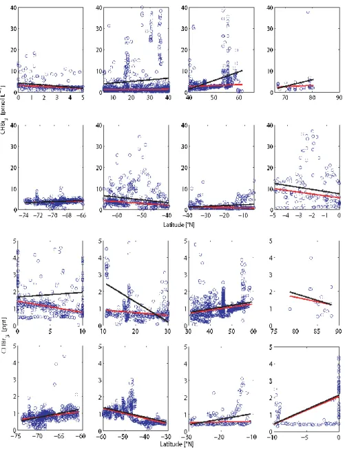
Fig. 2. Latitudinal distribution of open ocean water (a) (pmol L−1) and atmosphere (b) (ppt) bromoform concentrations (blue circles) clas-sified in eight different latitudinal bands. The robust fit (RF) (red line) and ordinary least squares (OLS) (black line) regression analyses are included.
3.5 Robust fit vs. ordinary least squares
In our study, two different regression techniques are applied. The ordinary least squares (OLS) technique contains the least squares method. This means that the sum of squared devia-tions between the empirical y values in the dataset and the predicted linear approximation is minimized.
The second method for calculating regression coefficients is the robust fit (RF) technique which is especially used for not normally distributed values. A regression analysis is bust if it is not sensitive to outliers. The calculation of the ro-bust coefficients is based on the iteratively reweighted least squares process. In the first iteration each data point has
equal weight and the model coefficients are estimated us-ing ordinary least squares. In the followus-ing iterations, the weighting of the data points is recalculated so that the dis-tant data points from the model regression from the previous iteration are given lower weight. This process continues until the model coefficients are within a predefined range. Our cal-culations are based on the most common general method of robust regression, the “M-estimation” introduced by Huber (1964).
Both regression methods are shown in Fig. 2 for all lat-itudinal divided open ocean water and atmospheric mea-surements for bromoform. The RF regression lines (red) are lower than the OLS (black) and occasionally show different
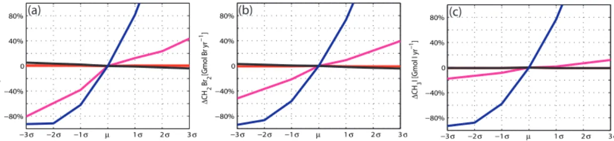
−3 −2 −1 1 2 3 −80% −40% 0 40% 80% ∆CHBr 3 [Gmol Br yr −1] σ σ σ µ σ σ σ −3 −2 −1 1 2 3 −80% −40% 0 40% 80% ∆CH 2 Br2 [Gmol Br yr − 1] σ σ σ µ σ σ σ −3 −2 −1 1 2 3 −80% −40% 0 40% 80% ∆CH 3 I [Gmol I yr −1] σ σ σ µ σ σ σ (a) (b) (c)
Fig. 3. The percentage change of the global oceanic emission for bromoform (a), dibromomethane (b), both in Gmol Br yr−1, and methyl iodide (c), in Gmol I yr−1, based on individual input parameters: wind speed (blue), sea surface temperature (magenta), sea surface salinity (red) and sea level pressure (black). The input parameters are individually increased and decreased by their multiple standard deviations (−3σ to 3σ ) while the other input parameters remain fixed (µ presents the oceanic emission using the mean input parameters).
trends. The reason for the large deviation between the RF and OLS regression is the different weighting of outliers. Out-liers crucially influence the value of the OLS slope, whereas the RF regression is located at the largest data density and reduces the influence of outliers. While the RF captures background values, the OLS technique indicates the variabil-ity of the data. Based on the obtained concentration maps, global fluxes are calculated and compared to literature values (see Supplement for a list of all calculated atmospheric and oceanic grid points based on linear regression and objective mapping as well as on linear regression only).
3.6 Air–sea gas exchange and input parameters
Fluxes (F in pmol cm h−1) across the sea–air interface are generally calculated as the product of the sea-to-air concentration difference and a gas exchange velocity. The partitioning of a gas between the water and gas phase is described by the dimensionless Henry’s law constant (H ) which highly depends on temperature and the molecular structure of the species. For our calculations, the Henry’s law constants of Moore et al. (1995a, b) are used. The at-mospheric mixing ratios (Cm in ppt) are converted to
equi-librium water concentrations (Ca in pmol L−1)and the
devi-ation from the actual measured water concentrdevi-ation (Cw in
pmol L−1)describes the driving concentration gradient. The sea-to-air flux is negative if the transport is from the atmo-sphere to the ocean.
F = k(Cw−CaH−1) (1)
Ca=Cm·SLP/(SST + 273.15)/83.137 (2)
H =exp(−4973/(SST + 273.15) + 13.16)for CHBr3 (3)
Several parameterizations for the air–sea gas exchange ex-ist in the literature, which express the relationship between the gas exchange velocity (k in cm h−1)and wind speed (e.g. Liss and Merlivat, 1986; Wanninkhof, 1992; Wanninkhof and McGillis, 1999; Nightingale et al., 2000). Experiments have shown that the dominant parameter influencing k is the wind speed. We chose to calculate the transfer coefficients based on the parameterization from Nightingale et al. (2000) with
corrections for the water temperature and a Schmidt num-ber (Sc) dependence for each gas (Quack and Wallace, 2003; Johnson, 2010).
k = (0.222U2+0.333U )sqrt(660Sc−1) (4)
The dimensionless Schmidt number is the ratio of the diffu-sion coefficient of the compound (D in cm2s−1)of interest and the kinematic viscosity (ν in cm2s−1)of sea water, and depends mainly on the temperature and the salinity.
Sc = ν/D (5)
D = (193 × 10−10×SST2+1686 × 10−10×SST (6)
+403.42 × 10⁻⁸)for CHBr3
The diffusion coefficients for the compounds were calculated according to Quack and Wallace (2003).
The gas exchange velocity and concentration gradient are dependent on SST, SSS, U and SLP as input parameters. During the initial stages of this study, we used climatologi-cal mean values (1989–2011) of the input parameters for our calculation of the global climatological emission estimates. A sensitivity study demonstrates how changes in the input parameters (climatological means) affect the global flux cal-culation for bromoform, dibromomethane and methyl iodide (Fig. 3). Each input parameter is individually increased and decreased by their multiple standard deviations (−3σ to 3σ ) while the other input parameters remain fixed. The standard deviations are calculated for every grid point for the years 1989–2011. This study shows the importance of each in-put parameter for the flux variance. Sea surface salinity and sea level pressure affects the VSLS emission calculations least compared with the other parameters (Fig. 3). Changes in wind speed and sea surface temperature have strong in-fluences on the bromoform sea-to-air flux. In general, a re-duction/enhancement of the wind speed is directly accom-panied by a decrease/increase in air–sea gas exchange co-efficients, and higher/lower sea surface temperature leads to an increase/decrease of the concentration gradients as well as the air–sea gas exchange coefficients (Schmidt number).
The dependencies of the global dibromomethane emission variability on the individual input parameters are the same as described for bromoform. The global methyl iodide emis-sions are mainly influenced by variations of the wind speed, while the other parameters have less effect. The sensitivity study shows that marginal changes of the input parameters can lead to a significant variation of the global flux estimate. Averaging over a long time period when producing clima-tological means involves smoothing extreme values, which is especially relevant for the wind speed (Bates and Merli-vat, 2001). Since the air–sea gas exchange coefficient has a non-linear dependence on wind speed, the application of av-eraged data fields causes a bias towards a lower flux when compared to using instantaneous winds and averaging the emission maps afterwards (Chapman et al., 2002; Kettle and Merchant, 2005). To reduce the bias, we apply the highest available temporal resolution of the input parameters and calculate 6-hourly global emissions with 6-hourly means of
U, SST, SLP and monthly means for the SSS (from January 1989 to December 2011). Finally, we sum the emissions for each month, calculate monthly average emissions over the twenty-one years and summarise these twelve averages to obtain the climatological annual emission.
4 Results and discussion
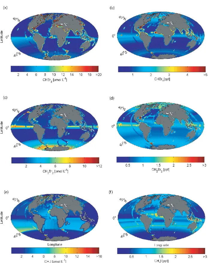
Marine (pmol L−1) and atmospheric (ppt) global surface concentration maps of bromoform, dibromomethane and methyl iodide calculated with the RF regression are shown in Fig. 4 (surface ocean concentrations and mixing ratios cal-culated with the OLS technique are illustrated in the Supple-ment). Based on the RF and OLS marine and atmospheric concentration maps, global sea-to-air flux climatologies are calculated (Fig. 5).
4.1 Climatological concentration maps of CHBr3 and
CH2Br2
Marine surface concentrations of bromoform (Fig. 4) are higher in the equatorial region (∼ 6 pmol L−1), upwelling ar-eas (e.g. the Mauritanian upwelling region ∼ 21 pmol L−1), near coastal areas (∼ 17–42 pmol L−1)and in shelf regions (∼ 8–32 pmol L−1), consistent with macroalgal and anthro-pogenic sources along the coast lines as well as biological sources in upwelling areas (Carpenter and Liss, 2000; Quack and Wallace, 2003; Yokouchi et al., 2005; Quack et al., 2007; Liu et al., 2011). The coastal and shelf areas both show a pos-itive latitudinal sea surface concentration gradient for bro-moform and dibromomethane towards the polar regions. The coastal sea surface concentrations of bromoform are on av-erage twice as high as in the shelf region. The open ocean generally has homogeneous concentrations between 0.5 and 4 pmol L−1. Lower values are located especially in the
sub-tropical gyres (∼ 0.5–1 pmol L−1), most distinctly in the At-lantic, North Pacific and southern Indian Ocean.
Estimating global concentration maps based on an identi-fied linear relationship is difficult in regions with sparse or missing data (e.g. Indian Ocean). Atlantic and Pacific Ocean data must be used to fill the data gap in the Indian Ocean, since no measurements exist there. Thus, we expect similar concentrations as in the other oceans. One dataset is available for the northern Indian Ocean (Yamamoto et al., 2001). The few measurements of bromoform in the Bay of Bengal are unusually high (> 50 pmol L−1)for an open ocean area. We decided to not include these outliers in our analysis, since our method would possibly overestimate water concentrations in the entire northern Indian Ocean using these data. The high concentrations in the equatorial region (the product of the other two basins) are approximately collocated with the upwelling season during the northeast monsoon, indicating higher productivity (Schott et al., 2002). The global ocean, and especially the Indian and Arctic, is data poor, and re-quires further sampling and evaluation to improve the predic-tions. Atmospheric surface mixing ratios of bromoform show similar distribution patterns. Higher atmospheric mixing ra-tios are located in the equatorial regions (1–3 ppt), around coastlines (∼ 1-10 ppt) and upwelling regions (10–17 ppt), as well as in the northern Atlantic (∼ 12–21 ppt), while lower mixing ratios are found above the subtropical gyres (∼ 0.2– 0.8 ppt).
The global surface oceanic concentration map of di-bromomethane shows similar patterns as bromoform. En-hanced oceanic surface concentrations are located around the equatorial region (∼ 6–9 pmol L−1), while low concen-trations occur in the subtropical gyres (1–2 pmol L−1), sim-ilar to CHBr3 in distribution, but with higher values.
Di-bromomethane concentrations in the coastal regions are sig-nificantly lower than those for bromoform. Distant from the coastal source regions CH2Br2 is mostly elevated in
the atmosphere relative to CHBr3, because it has a longer
atmospheric lifetime than CHBr3 (e.g. Brinckmann et al.,
2012) (CH2Br2=0.33 yr, CHBr3=0.07 yr, (Warneck and
Williams, 2012).
Elevated marine dibromomethane concentrations are found in the Southern Ocean (4–6 pmol L−1). This area is characterized by several circumpolar currents separated by frontal systems, with seasonally varying ice coverage, and is known to experience enhanced biological production (Smith and Nelson, 1985). Sea-ice retreat and the onset of microal-gae blooms have been related to an increase in marine surface bromocarbon concentrations (Hughes et al., 2009). However, this strong increase of CH2Br2is currently not understood.
The climatological maps represent annual average values that may underestimate seasonal and short-term variations (Hepach et al., 2013; Fuhlbr¨ugge et al., 2013). These varia-tions currently cannot be reflected in the model, since knowl-edge about production processes and the influence of envi-ronmental values on the concentrations is incomplete.
4.2 Climatological concentration maps of CH3I
The same classification and interpolation technique used for the bromocarbons reveal elevated marine and atmospheric concentrations of methyl iodide (2–9 pmol L−1, 0.3–1.5 ppt) in the subtropical gyre regions of both hemispheres (Fig. 4). This is in contrast to the oceanic concentration maps of bro-moform and dibromomethane, and is in agreement with re-ported production processes, such as photochemical oxida-tion of dissolved organic matter and iodide, as well as pro-duction from cyanobacteria (e.g. Richter and Wallace, 2004; Smythe-Wright et al., 2006).
Additionally, enhanced oceanic concentrations and at-mospheric mixing ratios are found in the upwelling re-gion off Mauritania and near the coastlines north of 40◦ (∼ 9 pmol L−1). Here in the region of offshore trade winds and dust export, the atmospheric methyl iodide from the ocean may be supplemented by input from land sources (Sive et al., 2007) as elevated air concentrations have been noted to be associated with dust events (Williams et al., 2007). The sharp concentration increase towards the coast, as ob-served for bromoform and dibromomethane, does not exist for methyl iodide. The open ocean concentrations are gen-erally higher than the coastal values, except for the North-ern Hemisphere. The elevated coastal oceanic concentrations might be due to the occurrence of macroalgae and anthro-pogenic land sources (e.g. Laturnus et al., 1998; Bondu et al., 2008) or to elevated levels of dissolved organic material (DOM) (e.g. Manley et al., 1992; Bell et al., 2002). The polar regions show generally homogenous and low concentrations of methyl iodide (Antarctic: ∼ 0.3 ppt, ∼ 1.5 pmol L−1; Arc-tic: ∼ 1 ppt and ∼ 0.3 pmol L−1).
4.3 Climatological emission maps of CHBr3and
CH2Br2
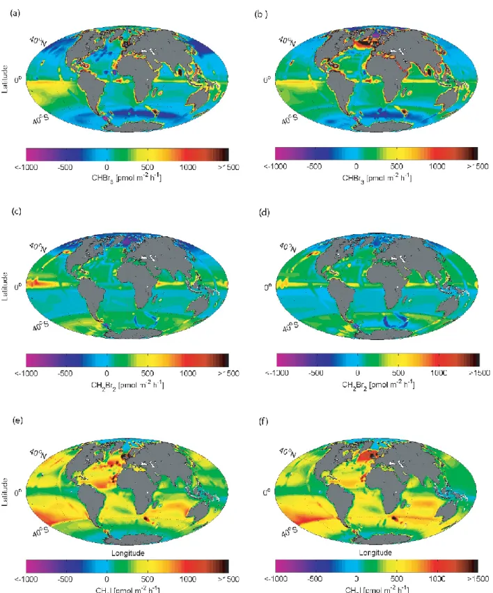
Elevated bromoform fluxes from the ocean to the atmo-sphere are generally found close to coastlines, in equato-rial and eastern boundary upwelling regions (e.g. the Mau-ritanian upwelling region) and a wide region of the south-ern Pacific (subtropical gyre). Very high sea-to-air fluxes (> 1500 pmol m−2h−1)also occur in the Bay of Bengal, the Gulf of Mexico, the North Sea and the east coast of North America.
While they cover 16 % of the world ocean area, the coastal and shelf regions, with their high biological produc-tivity, have enhanced concentrations of bromoform and di-bromomethane and account for 67/78(RF/OLS) % of total Br emission attributable to CHBr3 and 22/24 % of that
at-tributable to CH2Br2. Most of the open ocean appears almost
in equilibrium with the atmosphere, especially in the subtrop-ical gyre regions. A CHBr3flux from the atmosphere to the
ocean is seen in the entire Southern Ocean, the northern part of the Pacific and in some parts of the North Atlantic (e.g. east of North America).
Our open ocean flux of CHBr3is about 25 % of the global
sea-to-air flux estimate, which is in agreement with the 20 % calculated by Butler et al. (2007) and the 33 % of Quack and Wallace (2003). This underlines that the coast and shelf re-gions play a significant role in the global bromoform budget. The tropics (20◦N to 20◦S, including open ocean, shelf and coastal area) represent the region with the highest bromoform emissions of 44/55 % (Table 3). This is in agreement with the top-down approach of 55.6 % between 20◦N to 20◦S pub-lished by Ordonez et al. (2012) and of 37.7 % for 10◦N to 10◦S from Liang et al. (2010). A decrease in the total emis-sion towards the polar region is visible. Hence, the tropics are a “hot spot” for bromoform emissions.
Comparable with the sea-to-air fluxes based on the RF analysis, the emissions using the OLS method shows en-hanced sea-to-air fluxes in the North Atlantic and all gyre regions, and an elevated sink in the Arctic region (Fig. 5). We estimate a global positive sea-to-air flux for CHBr3 of ∼ 2.06 Gmol Br yr−1 (RF), ∼ 2.96 Gmol Br yr−1
(OLS); and a global sink, air-to-sea flux, for CHBr3 of
∼0.56 Gmol Br yr−1(RF), ∼ 0.47 Gmol Br yr−1(OLS). Differences between the distribution of source and sink re-gions and of CH2Br2emissions calculated with the RF and
OLS regression are less pronounced than those of CHBr3
(Fig. 5). The Arctic Ocean acts mainly as a sink for atmo-spheric CH2Br2, most likely because of the low sea surface
temperatures, low water concentrations and higher air con-centrations. The Southern Ocean (south of 50◦S) acts as a source to the atmosphere. The OLS based emissions show an enhanced source region in the southern Pacific due to elevated marine surface concentrations. We estimate a pos-itive global CH2Br2 sea-to-air flux of ∼ 0.89 Gmol Br yr−1
(RF), ∼ 1.09 Gmol Br yr−1(OLS); and an air-to-sea flux of
∼0.12 Gmol Br yr−1(RF), ∼ 0.11 Gmol Br yr−1(OLS). Our total open ocean flux of 0.6–0.76 Gmol Br (CH2Br2) yr−1 is in agreement with the estimates
of ∼ 0.7 Gmol Br yr−1given by Ko et al. (2003) and 0.6 Gmol Br yr−1 given by Butler et al. (2007). The coast and shelf regions play a minor role for the global CH2Br2
budget compared to the open ocean, which contributes
∼77 % Gmol Br yr−1. The global emission distribution for CH2Br2 and CHBr3 is similar in the midlatitudes and the
tropics. (Table 3). Enhanced source regions for the atmo-sphere are found in the tropical area contributing about 44/49 % between 20◦N and 20◦S. This is lower compared with the study of Ordonez et al. (2012) who calculated a con-tribution of 63.1 % from 20◦N to 20◦S. The CH
2Br2
emis-sions decrease towards the polar regions.
4.4 Climatological emission maps of CH3I
The global emissions of CH3I reveal an opposite pattern
compared with CHBr3and CH2Br2(Fig. 5). The main
dif-ference is the enhanced emission in the subtropical gyre re-gions.
Fig. 4. Global maps of marine concentrations (pmol L−1)and atmospheric mixing ratios (ppt) for bromoform (a, b), dibromomethane (c, d) and methyl iodide (e, f) based on the robust fit (RF) regression analyses. The concentration maps calculated with the OLS method are included in the Supplement (Fig. S3).
Fig. 5. Global sea-to-air flux climatology of bromoform (a, b), dibromomethane (c, d) and methyl iodide (e, f) in pmol m−2h−1based on the RF (a, c, e, left column) and OLS (b, d, f, right column) analyses.
Equatorial upwelling regions, as well as the Arctic and Antarctic polar regions, are mostly in equilibrium. In com-parison with CHBr3and CH2Br2, the global CH3I sea-to-air
fluxes are generally positive, indicating the larger supersat-urations of the oceanic waters. The OLS regression shows the North Atlantic to be a very strong source region for at-mospheric methyl iodide. Coast and shelf regions transport only ∼ 13 % of I (CH3I) to the atmosphere. The open ocean
contribution of 87 % is more than the estimate from Butler et al. (2007) of 50 % open ocean emissions of methyl iodide. Possibly, the subtropical gyre regions are more distinctive source areas in our climatology than in Butler et al. (2007). The southern tropics and subtropics represent the regions with the highest emission strength, decreasing towards the polar areas (Table 3). We calculate a global sea-to-air flux for CH3I of ∼ 1.24 Gmol I yr−1(RF) and ∼ 1.45 Gmol I yr−1
(OLS).
4.5 Evaluation of RF and OLS results
All subtropical regions, and especially the equator, show a large temporal and spatial variability in the data, which is re-flected in the enhanced RMSE parameter (Tables S1 and S2 in the Supplement). The wide concentration ranges might be caused by real variations between sampling in different sea-sons, where the seasonally varying strength and expansion of upwelling (equatorial and coastal) (Minas et al., 1982; Hagen et al., 2001) and solar flux may cause different concentrations of the compounds.
The evaluation of the two regression methods shows that RF is more representative of a climatology, since it is cal-culating a regression independently of outliers and weighted by the data distribution. In comparison, the OLS regression weights outliers, and, hence considers extreme data and vari-ability more than the RF method (Fig. 2). The global appear-ances of RF and OLS maps are not extremely different (see Supplement). Nevertheless, they introduce slight differences in the concentration gradients and in the sea-to-air flux cli-matologies.
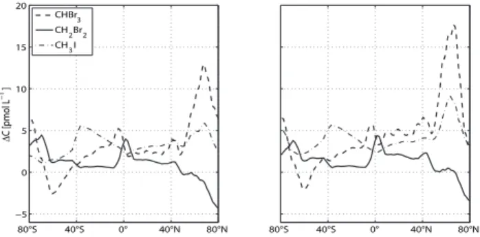
The influence of the RF and the OLS regression for the global surface concentration distribution in atmosphere and ocean, which has consequences for the concentration gra-dient, is shown in Table 1 and Fig. 6. In general, the OLS technique calculates higher mean and median values, includ-ing the enhanced concentrations and outliers. Additionally, bromoform shows higher variance compared with the other compounds in both techniques and reflects the high data vari-ability between coastal and open ocean bromoform concen-trations. Further, the calculated concentration gradient from the OLS method exhibits stronger source (emission into the atmosphere) and weaker sink regions compared with RF, which is again most pronounced for bromoform (Fig. 6). The OLS and RF distribution (mean, median and standard devi-ation) for dibromomethane and methyl iodide are in closer agreement compared with bromoform. The reason for this
80°S 40°S 0° 40°N 80°N −5 0 5 10 15 20 ∆C [pmol L −1] CHBr3 CH2Br2 CH 3I 80°S 40°S 0° 40°N 80°N
Fig. 6. Zonal mean concentration gradients for bromoform (dashed line), dibromomethane (solid line) and methyl iodide (dash-dotted line) in pmol L−1, calculated with RF (left side) and OLS (right side) methods.
smaller difference between RF and OLS is the occurrence of less extreme values in the concentration gradients for CH2Br2and CH3I compared with CHBr3. The global surface
emissions of bromoform, dibromomethane and methyl io-dide yield a similar spatial distribution with both techniques (Table 2).
4.6 Comparison of estimation methods
In the following section we compare our emission clima-tology with recently published estimates, including differ-ent calculation techniques (i.e. bottom-up and top-down ap-proaches), as well as laboratory experiments (Table 6). The global bromoform emission estimates show the largest dif-ference between the studies.
Warwick et al. (2006) modelled surface mixing ratios us-ing different emission scenarios and fitted them to the avail-able atmospheric measurements. These scenarios applied different global emission estimates, e.g. the bottom-up es-timate from Quack and Wallace (2003). The course resolu-tion of 2.8◦×2.8◦used in the Warwick study does not well resolve the coastal areas, which are thought to be the main source for bromoform. In addition the applied uniform inter-polations do not reflect the actual conditions. In the results of Warwick et al. (2006), the coastlines further north and south of the tropics exhibit no enhanced atmospheric bromoform concentrations or emission to the atmosphere compared to the open ocean. This does not reflect the in situ measure-ments from the HalOcAt database. Based on local bromo-form measurements in Southeast Asia, Pyle et al. (2011) re-duced the emission estimate of Warwick et al. (2006) in this coastal area. This study shows the importance of local mea-surements for the improvement of global estimates. Other model studies based on the ideas of Warwick et al. (2006), e.g. Kerkweg et al. (2008), show the same underestimation of coastal emissions in the extra tropics. In contrast, Liang et al. (2010) consider all coastlines with enhanced emissions in their scenario; furthermore the finer classification of their emission scenario compared with Warwick et al. (2006) is
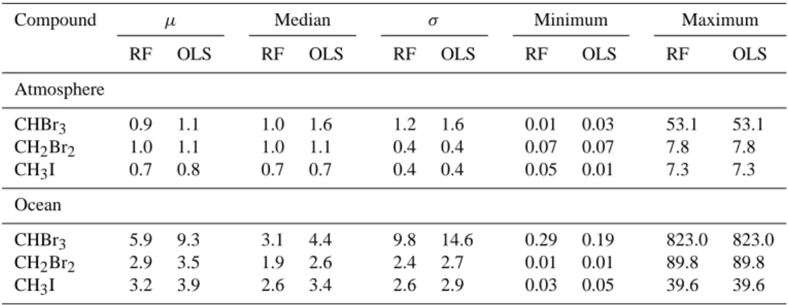
Table 1. Statistical moments: mean (µ), median, standard deviation (σ ), minimum and maximum values of atmospheric mixing ratio (ppt) and oceanic concentration (pmol L−1)climatologies of CHBr3, CH2Br2and CH3I based on the RF and OLS regression analyses.
Compound µ Median σ Minimum Maximum
RF OLS RF OLS RF OLS RF OLS RF OLS
Atmosphere CHBr3 0.9 1.1 1.0 1.6 1.2 1.6 0.01 0.03 53.1 53.1 CH2Br2 1.0 1.1 1.0 1.1 0.4 0.4 0.07 0.07 7.8 7.8 CH3I 0.7 0.8 0.7 0.7 0.4 0.4 0.05 0.01 7.3 7.3 Ocean CHBr3 5.9 9.3 3.1 4.4 9.8 14.6 0.29 0.19 823.0 823.0 CH2Br2 2.9 3.5 1.9 2.6 2.4 2.7 0.01 0.01 89.8 89.8 CH3I 3.2 3.9 2.6 3.4 2.6 2.9 0.03 0.05 39.6 39.6
Table 2. Statistical moments: mean (µ), median, standard deviation (σ ), minimum and maximum values for the calculated global sea-to-air flux climatologies of CHBr3, CH2Br2and CH3I based on the RF and OLS regression analyses, in pmol m−2h−1.
Global Sea-to-Air µ Median σ Minimum Maximum
Flux Climatology RF OLS RF OLS RF OLS RF OLS RF OLS
CHBr3 154.9 236.2 47.1 89.7 549.7 749.6 −5339 −5230 19 618 19 618
CH2Br2 76.5 112.4 79.3 78.8 237.9 258.4 −1687 −1714 3978 3978
CH3I 329.6 405.0 307.3 385.2 289.8 348.3 −49 −55 4895 4878
Table 3. The emission distribution of CHBr3, CH2Br2and CH3I
calculated with two different regression methods (RF and OLS) for different latitudinal bands (see text for explanation), expressed as a percentage.
CHBr3 CH2Br2 CH3I
RF OLS RF OLS RF OLS
50–90◦N 22.8 21.2 −9.7 −4.9 10.4 7.6
20–50◦N 7.4 15.9 13.7 19.1 19.8 20.3
20◦N–20◦S 54.7 43.6 48.9 44.3 28.9 32.1
20–50◦S 22.7 19.3 25.1 22.1 32.8 34.1
50–90◦S −7.6 0.007 22.0 19.5 8.2 5.9
similar to our study. Another comparable classification (lat-itudinal bands, higher emissions in coastal regions) is used in the model (top-down approach) by Ordonez et al. (2012), who parameterized oceanic polybromomethanes emissions based on a chlorophyll a (chl a) dependent source in the tropical ocean (20◦N to 20◦S). We also see the occurrence of
enhanced bromoform, as well as dibromomethane emissions in tropical upwelling regions and in coastal regions, although a direct correlation between chl a and the VSLS compounds is not apparent from the observations (Abrahamsson et al., 2004; Quack et al., 2007b). Palmer and Reason (2009) devel-oped a parameterization for CHBr3based on chl a (between
30◦N and 30◦S), including other parameters (mixed layer depth, sea surface temperature and salinity, wind speed). The
correlation between his modelled values and observations is, with r2=0.4, low, which reveals the deficiency of this method (and chl a).
In some studies local emission estimates are extrap-olated to a global scale. Extrapolating near-shore emis-sions may significantly overestimate the global sea-to-air fluxes, since they generally include elevated coastal con-centrations, which are not representative of the global ocean. Yokouchi et al. (2005) applied a coastal emission ratio of CHBr3/CH2Br2 of 9, and a global emission of
0.76 Gmol Br yr−1for CH2Br2to infer a global CHBr3flux
estimate of 10.26 ± 3.88 Gmol Br yr−1. O’Brien et al. (2009) followed the same method and extrapolated local near-shore measurements in the region surrounding Cape Verde to a global scale using an emission ratio of CHBr3/CH2Br2=13.
The global fluxes from these studies are nearly four times higher than those calculated in our study. However, since the emission ratios of CHBr3to CH2Br2are generally higher in
coastal regions than in the other areas (Hepach et al., 2013), the calculated global flux for CHBr3could be an
overestima-tion.
Butler et al. (2007) and Quack and Wallace (2003) inter-polated oceanic and atmospheric in situ measurements for global emission estimates. Butler et al. (2007) subdivided the ocean into the main basins and calculated the fraction of each compound for each region as a percentage. Coastal areas were not considered. The extrapolation by Quack and Wallace (2003) contained most of the currently available
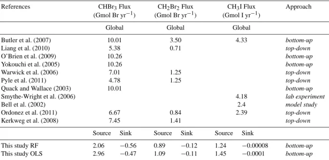
Table 4. Fluxes of bromine from CHBr3and CH2Br2in Gmol Br yr−1, and iodine from CH3I in Gmol I yr−1.
References CHBr3Flux CH2Br2Flux CH3I Flux Approach
(Gmol Br yr−1) (Gmol Br yr−1) (Gmol I yr−1)
Global Global Global
Butler et al. (2007) 10.01 3.50 4.33 bottom-up
Liang et al. (2010) 5.38 0.71 top-down
O’Brien et al. (2009) 10.26 bottom-up
Yokouchi et al. (2005) 10.26 bottom-up
Warwick et al. (2006) 7.01 1.25 top-down
Pyle et al. (2011) 4.78 1.25 top-down
Quack and Wallace (2003) 10.01 bottom-up
Smythe-Wright et al. (2006) 4.18 lab experiment
Bell et al. (2002) 2.4 model study
Ordonez et al. (2011) 6.67 0.84 2.39 top-down
Kerkweg et al. (2008) 7.45 1.41 top-down
Source Sink Source Sink Source Sink
This study RF 2.06 −0.56 0.89 −0.12 1.24 −0.00008 bottom-up
This study OLS 2.96 −0.47 1.09 −0.11 1.45 −0.0001 bottom-up
Fig. 7. Inter-annual sea-to-air flux variability over 1989–2011 (bold solid line) of bromoform (left), dibromomethane (centre) and methyl iodide (right) calculated with the two regression techniques (RF (lower panels) and OLS (upper panels)), in Gmol (Br/I) yr−1. Additionally, the respective climatological value is marked (dash-dotted line) as well as the standard deviation (grey shaded).
published measurements and used a finer area classification for shore, shelf and open ocean regions as well as for lati-tudinal bands. Both bottom-up approaches applied a coarse data interpolation compared to the classification and regres-sion techniques used in this study and appear too high.
We calculate a global CH2Br2 sea-to-air flux of 0.77–
0.98 Gmol Br yr−1, which is also in the lower (0.71– 3.5 Gmol Br yr−1)range of the other estimates (Table 4), but is in much closer agreement compared to the other com-pounds. Reasons for the good agreement with recent stud-ies could be the longer atmospheric lifetime of CH2Br2and
the lower variance of sea water values which cause a more homogenous global distribution.
Some earlier emission estimations for CH3I (1.05–
10.5 Gmol I yr−1)are given by Bell et al. (2002), who
pro-duced the first seasonal model simulation of global oceanic and atmospheric CH3I surface concentrations. A low
corre-lation between observations and modelled data was obtained (r = 0.4). The authors assumed a missing biological sink of CH3I in the ocean that would have reduced their
com-puted concentrations to better match the observations. Sink and source mechanisms for the formation of CH3I are not
fully understood, making it difficult to model CH3I emissions
based on source and sink parameterizations. In our study a global sea-to-air flux of 1.24–1.45 Gmol I yr−1is estimated, which is within the lower range of earlier studies (Table 4). Our calculated climatology uses a larger dataset than the study of Bell et al. (2002). Ordonez et al. (2012) calculate a global CH3I flux of the same magnitude as our study
us-ing a top-down approach with a modified global chemistry model that includes bromine and iodine chemistry. Smythe-Wright et al. (2006) calculated a global flux of iodine from Prochlorococcus marinus of ∼ 4.18 Gmol I yr−1 based on measurements from two cruises. The latter study assumes that this phytoplankton species is the major marine source of atmospheric CH3I. The assumption of Smythe-Wright et
al. (2006) that the oceanic surface (< 40◦N and S) is cov-ered with CH3I-producing picoplankton might overestimate
the global CH3I sea-to-air flux. Calculations based on culture
experiments from Brownell et al. (2010) demonstrate that Prochlorococcus marinus accounts only for 0.03 % of the global CH3I budget and is not a globally significant source
of CH3I. Hughes et al. (2011) suggest different culture
con-ditions as a possible explanation for the contradictory find-ings of the culture experiments. The bottle experiments of
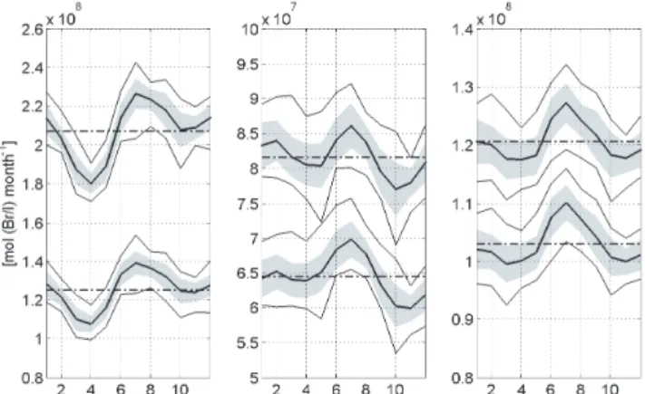
Fig. 8. Global monthly sea-to-air flux averages of bromoform (left), dibromomethane (centre) and methyl iodide (right) in mol (Br/I) month−1(bold solid line) from 1989 to 2011, including their stan-dard deviation (grey shaded area) and their minimum and maximum value (solid line). Additionally, the respective annual mean value is marked (dash-dotted line). The upper graphs show the oceanic emis-sions using the OLS regression technique and the bottom graphs the RF calculated fluxes.
Richter and Wallace (2004) suggested a photochemical pro-duction pathway of CH3I in open ocean water which might
also explain our surface distribution (enhanced emissions in the subtropical gyre regions).
The comparison of our global sea-to-air fluxes with other global estimates reveals the greatest discrepancy for bromo-form. We have shown that bromoform levels are the most variable in the ocean and atmosphere. Possibly, the under-representation of extreme values generates too small concen-tration gradients, which reduces our total emission estimate. Especially in coastal and shelf regions, the 1◦×1◦grid
reso-lution cannot resolve these extreme concentrations and very likely leads to underestimated emissions.
5 Variability of the climatological sea-to-air fluxes
We calculate global emission fields using fixed oceanic con-centrations and atmospheric mixing ratios and the highest available temporal resolution of the input parameters over the time period 1989–2011: 6-hourly means of U , SST, SLP and monthly means for the SSS. The global emissions of ev-ery time step are averaged over each month and the average monthly emissions are summed to the annual climatologi-cal emission. The climatologies thus include annual, seasonal and short timescale temporal variability.
5.1 Variability of the concentration data
The calculated global 1◦×1◦ maps of oceanic concentra-tions and atmospheric mixing ratios include in situ measure-ments from 1989 to 2011, illustrating a climatological year and covering the entire globe. Seasonally changing
condi-tions, e.g. light and water temperature or biological species composition, which have an influence on the variability of the air and water concentrations in certain areas (Archer et al., 2007; Orlikowska and Schulz-Bull, 2009), are not con-sidered because of the generally poor temporal data cover-age. Fitting the in situ measurements onto our 1◦×1◦grid (by using objective mapping) leads on average to a reduction of the initial atmospheric mixing ratios and oceanic concen-trations of less than 1 %. The accuracy of the interpolation is limited by the sparse data coverage and the regression tech-nique used. Seasonal and spatial accuracy could be improved if a larger dataset was available. Thus we recommend more measurements, especially in the ocean, as well as a refine-ment of process understanding. The temporal variability of the SST is considered in the concentration gradient, used in the sea-to-air flux calculation, by computing a new equilib-rium concentration for every 6 h time step from 1989 to 2011.
5.2 Annual and seasonal variability
The inter-annual variability of the global sea-to-air flux from 1989 to 2011 is small and generally less than 5 % (Fig. 7). The halocarbons all show a positive trend towards 2011. Within a year, the global flux varies monthly for every halo-genated compound (Fig. 8). The maximum global sea-to-air flux is most pronounced in July for all compounds, while the minimum is reached in March–April for CHBr3 and CH3I
and in October for CH2Br2. The climatological monthly
flux and the corresponding minimum and maximum monthly fluxes vary between 9 and 21 %. CH3I shows the smallest
mean deviation with 9 and 11 % for OLS and RF respec-tively, whereas the variation for CH2Br2is between 14 and
17 % and for CHBr3 between 17 and 21 %. Thus the
sea-sonal variation of the global climatological flux is larger than the inter-annual variation, despite the shifting of the seasons (half a year) between the Northern Hemisphere and Southern Hemisphere. The global climatological fluxes, obtained from the sum of the monthly averages between 1989 and 2011, de-scribe the current best possible estimates of the moderately varying annual and seasonal global emissions. However, the results do not consider a seasonally varying influence of ei-ther the water or the air concentration on the emission be-cause the current sparse investigations do not allow a suitable parameterization of the VSLS yet.
5.3 Short time variability of fluxes
In situ fluxes from a cruise (TransBrom) between Japan and Australia in October 2009 are compared to the near-est grid points of our climatology (Fig. 9) as an example for the influence of short time variability. The TransBrom data include 105 CHBr3 and CH2Br2 measurements and
96 CH3I measurements, and are included in the
climatol-ogy. The cruise transited through different biogeochemical regions with varying meteorological conditions influencing
(a) (b) (c)
(d) (e) (f)
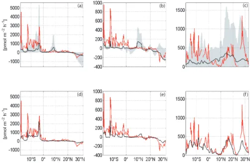
Fig. 9. The upper panels illustrate the comparison between our climatological estimate (black line) and the in situ sea-to-air fluxes from the TransBrom cruise (red line) for bromoform (a), dibromomethane (b) and methyl iodide (c) in pmol m−2h−1(see more details in the text) including the climatological minimum and maximum values (grey shaded area). The lower panels represent the same in situ measurements compared to our model values using the nearest 6-hourly mean of SST, U and SLP and monthly mean of SSS with fixed mixing ratios and oceanic concentrations calculated with the RF method for bromoform (d), dibromomethane (e) and methyl iodide (f) (the emissions using OLS look similar).
the strength of VSLS emissions (Kr¨uger and Quack, 2012). The in situ and climatological sea-to-air fluxes for bro-moform and dibromomethane compare very well in the Northern Hemisphere, where small concentration gradients are found in the open oceans. The enhanced emissions in the Southern Hemisphere encountered during the cruise are under-represented in the climatology. Comparison of the methyl iodide in situ fluxes and the climatology shows a sim-ilar trend, although the extreme values of the in situ mea-surements are highly under-represented in the climatological mean flux value. Our climatology underestimates the short-term measured fluxes by smoothing the values of the varying input parameters. The mean deviation between the climatol-ogy and the in situ fluxes during October 2009 is ∼ 120 % for CHBr3, ∼ 20 % for CH2Br2and ∼ 176 % for CH3I,
respec-tively.
We also calculate the sea-to-air fluxes using the nearest temporal and spatial 6-hourly means (highest available reso-lution) of SST, SLP and U , the monthly mean of the SSS and the climatological oceanic concentration and mixing ratios, and compare them to the measured fluxes (Fig. 9). The mean deviation between the 6-hourly means and the in situ fluxes for the three compounds is only ∼ 48 % for CHBr3, ∼ 15 %
for CH2Br2and 51 % for CH3I. These values show the good
match between “modelled” and in situ measurements and validate the predictive capability of this approach. The cli-matological minimum and maximum values of the cruise
nearest data points (Fig. 9, upper panel) reveal how variable the “modelled” fluxes can be at a single location. While most in situ fluxes are included in the 6 h minimum and maximum range from 1989 to 2011, it is also noteworthy that even with this high temporal (6 h) resolution of input parameters, the “modelled” fluxes can neither match the extreme values of the encountered in situ fluxes, nor do they resolve the high variability of the in situ fluxes completely. An additional fac-tor for the under-representation of the extreme in situ values is the mean concentration gradient (1◦×1◦resolution) in our
“model”. In the vicinity of source regions, e.g. coast lines, the water concentrations can vary by more than 100 % over short distances (Butler et al., 2006), which strongly influences the in situ fluxes and is likely not resolved in the model due to poor data coverage.
6 Summary and conclusion
Global sea-to-air flux climatologies (considering the time span from 1989 to 2011 of the three important short-lived halocarbons, bromoform, dibromomethane and methyl io-dide) are calculated based on surface oceanic and atmo-spheric measurements from the HalOcAt database. The phys-ical and biogeochemphys-ical factors of the compounds’ distribu-tions in ocean and atmosphere are also considered. Data are classified into coastal, shelf and open ocean regions, and are interpolated on a 1◦×1◦ grid. The missing grid values are
filled with robust fit (RF) and ordinary least squares (OLS) regression techniques based on the latitudinal and longitudi-nal distribution of the compounds. The RF interpolation esti-mates background values, since it is weighted on the quantity of measurements, whereas the OLS regressions include ex-treme data and therefore represent our highest values. Global emission fields are calculated with a high temporal resolution of 6-hourly wind speed, sea surface temperature and sea level pressure data. The climatological annual global flux for 1989 to 2011 is obtained as sum of the monthly average fluxes. We estimate positive global sea-to-air fluxes of CHBr3,
CH2Br2and CH3I of 2.06/2.96, 0.89/1.09 Gmol Br yr−1and
1.24/1.45 Gmol I yr−1, based on RF/OLS respectively, which are all at the lower end of earlier studies. Previous global cli-matological estimate studies have not determined negative fluxes (flux into the ocean). We estimate negative global sea-to-air fluxes of −0.47/−0.56, −0.11/−0.12 Gmol Br yr−1 and −0.08/−0.1 Mmol I yr−1for CHBr3, CH2Br2and CH3I,
respectively. The net oceanic emissions of our climatology are 1.5/2.5 Gmol Br yr−1for CHBr3, 0.78/0.98 Gmol Br yr−1
for CH2Br2, and 1.24/1.45 Gmol I yr−1for CH3I.
Our low bottom-up emission estimates, compared to re-cent top-down approaches, especially for bromoform, are most likely caused by an under-representation of extreme emissions. Observed high temporal and spatial in situ vari-ances cannot be resolved in the 1◦×1◦ grid climatology. It is still unclear how important extreme events are for the global bromoform budget, but we suggest that small spatial and temporal events of high oceanic bromoform emissions are important for the transport of bromine into the tropo-sphere and lower stratotropo-sphere. The monthly variation of the global climatological flux (9–21 %) is contained within our calculations and it is larger than the inter-annual variability, which is generally less than 5 % for all three compounds.
Our global sea-to-air flux estimates can be used as input for different model calculations. The existing uncertainties can be reduced by enlarging of the HalOcAt database with more measurements, especially in ocean waters, common calibration techniques and more basic research into the un-derlying source and sink processes.
Supplementary material related to this article is
available online at: http://www.atmos-chem-phys.net/13/ 8915/2013/acp-13-8915-2013-supplement.zip.
Acknowledgements. We thank all contributors sending their
data to the HalOcAt database and for their helpful comments on the manuscript. We also thank our assisting student helpers Julian Kinzel, Christian M¨uller, Eike H¨umpel, Anja M¨uller and Theresa Conradi who populated the database, which started in 2009. This work was financially supported by the WGL project TransBrom, the European commission under the project SHIVA
(grant no. 226 224) and by the German Federal Ministry of Education and Research (BMBF) during the project SOPRAN (grant no: 03F0611A). SOLAS Integration (Surface Ocean Lower Atmosphere Study; http://www.bodc.ac.uk/solas integration/) helped instigate this project and Tom Bell and Peter Liss were supported in this by a NERC UK SOLAS Knowledge Transfer grant (NE/E001696/1). Part of this project was supported by COST (European Cooperation in Science and Technology) Action 735, a European Science Foundation-supported initiative. Additionally, we would like to thank the ECMWF for providing the ERA Interim reanalysis data. We thank two anonymous reviewers for their useful comments and advice.
The service charges for this open access publication have been covered by a Research Centre of the Helmholtz Association.
Edited by: R. Volkamer
References
Abrahamsson, K., Bertilsson, S., Chierici, M., Fransson, A., Froneman, P. W., Loren, A., and Pakhomov, E. A.: Varia-tions of biochemical parameters along a transect in the south-ern ocean, with special emphasis on volatile halogenated or-ganic compounds, Deep-Sea Res. Part II, 51, 2745–2756, doi:10.1016/j.dsr2.2004.09.004, 2004.
Amachi, S., Kamagata, Y., Kanagawa, T., and Muramatsu, Y.: Bacteria mediate methylation of iodine in marine and terres-trial environments, Appl. Environ. Microbiol., 67, 2718–2722, doi:10.1128/aem.67.6.2718-2722.2001, 2001.
Antonov, J. I., Seidov, D., Boyer, T. P., Locarnini, R. A., Mishonov, A. V., Garcia, H. E., Baranova, O. K., Zweng, M. M., and John-son, D. R.: World ocean atlas 2009, Volume 2: Salinity. S. Levitus Ed. NOAA Atlas NESDIS 69, U.S. Government Printing Office, Washington, DC, 184 pp., 2010.
Archer, S. D., Goldson, L. E., Liddicoat, M. I., Cummings, D. G., and Nightingale, P. D.: Marked seasonality in the concentrations and sea-to-air flux of volatile iodocarbon compounds in the west-ern English Channel, J. Geophys. Res.-Oceans, 112, C08009, doi:10.1029/2006jc003963, 2007.
Aschmann, J., Sinnhuber, B.-M., Atlas, E. L., and Schauffler, S. M.: Modeling the transport of very short-lived substances into the tropical upper troposphere and lower stratosphere, Atmos. Chem. Phys., 9, 9237–9247, doi:10.5194/acp-9-9237-2009, 2009. Bates, N. R. and Merlivat, L.: The influence of short-term wind
vari-ability on air-sea CO2exchange, Geophys. Res. Lett., 28, 3281–
3284, doi:10.1029/2001gl012897, 2001.
Bell, N., Hsu, L., Jacob, D. J., Schultz, M. G., Blake, D. R., Butler, J. H., King, D. B., Lobert, J. M., and Maier-Reimer, E.: Methyl iodide: Atmospheric budget and use as a tracer of marine con-vection in global models, J. Geophys. Res.-Atmos., 107, 4340, doi:10.1029/2001jd001151, 2002.
Bondu, S., Cocquempot, B., Deslandes, E., and Morin, P.: Effects of salt and light stress on the release of volatile halogenated organic compounds by Solieria Chordalis: A laboratory incubation study, Bot. Mar., 51, 485–492, doi:10.1515/bot.2008.056, 2008. Brinckmann, S., Engel, A., B¨onisch, H., Quack, B., and Atlas,