HAL Id: tel-02860058
https://tel.archives-ouvertes.fr/tel-02860058
Submitted on 8 Jun 2020HAL is a multi-disciplinary open access archive for the deposit and dissemination of sci-entific research documents, whether they are pub-lished or not. The documents may come from
L’archive ouverte pluridisciplinaire HAL, est destinée au dépôt et à la diffusion de documents scientifiques de niveau recherche, publiés ou non, émanant des établissements d’enseignement et de
Chi-Hak Uy
To cite this version:
Chi-Hak Uy. Two-Polarization dynamics in optically delayed lasers. Optics / Photonic. Centrale-Supélec, 2018. English. �NNT : 2018CSUP0006�. �tel-02860058�
CentraleSupélec
Ecole Doctorale
C2MP
« Chimie Mécanique. Matériaux Physique »
Laboratoire LMOPS
« Laboratoire Matériaux Optiques, Photonique et Systèmes »
THÈSE DE DOCTORAT
DOMAINE : SPI
Spécialité : Photonique
Soutenue le
31 octobre 2018
par :
Chi-Hak UY
Two-Polarization dynamics in optically delayed lasers
Composition du jury :
Directeur de thèse : Marc SCIAMANNA Professeur, CentraleSupélec
Co-directeur de thèse : Damien RONTANI Maître de conférences, CentraleSupélec
Rapporteurs : Frédéric GRILLOT Professeur, Télécom ParisTech Krassimir PANAJOTOV Professeur, Vrije Universiteit Brussel Examinateurs : Stefan BREUER Dr. Habil., Technische Universität Darmstadt
Cristina DE DIOS FERNANDEZ Professeur, Universidad Carlos III de Madrid Germano MONTEMEZZANI Professeur, Université de Lorraine
Page
1 Introduction 1
1.1 From maser to laser : the story of Charles H. Townes . . . 2
1.2 Physics of lasers . . . 6
1.2.1 Principle . . . 6
1.2.2 Semiconductor lasers . . . 9
1.2.3 From edge to surface-emitting lasers . . . 11
1.2.4 Relaxation oscillations . . . 12
1.3 Some Applications of lasers . . . 14
1.3.1 Optical communications . . . 14
1.3.2 LIDAR for optical ranging and aerosol detection . . . 15
1.4 Nonlinear dynamics and chaos in laser diodes . . . 16
1.4.1 The strange-attractor of Lorenz . . . 17
1.4.2 Bifurcation diagram of the Lorenz’s equations . . . 19
1.4.3 Analogy between lasers and the Lorenz’s system . . . 21
1.4.4 Classification of lasers . . . 23
1.4.4.1 Class C lasers . . . 23
1.4.4.2 Class B lasers . . . 24
1.4.4.3 Class A lasers . . . 24
1.4.5 Unlocking nonlinear dynamics in semiconductor lasers . . . 24
1.4.5.1 Different approaches . . . 24
1.4.5.2 Optical feedback and route to chaos . . . 26
1.5 Applications of chaos in laser diodes . . . 29
1.5.1 Chaos for secure communication . . . 29
1.6 Conclusion, objectives and outlines . . . 31
2 Polarization instabilities in VCSELs and non-local correlation prop-erty in low-frequency fluctuation regime 33 2.1 Polarization properties in VCSELs . . . 34
2.1.1 Polarization instabilities in VCSELs in comparison with EELs 35 2.1.2 Types of polarization switching . . . 36
2.1.2.1 Polarization selection from gain competition . . . 37
2.1.2.2 Polarization selection from gain competition and losses 39 2.1.3 Prediction of polarization switching from spin relaxation process 41 2.1.4 Application of polarization instabilities . . . 45
2.1.4.1 Random bits generation . . . 45
2.1.4.2 Logical gates . . . 46
2.1.4.3 High-frequency oscillation generation . . . 47
2.1.4.4 Reservoir computing based on two polarization modes 47 2.2 VCSEL under optical feedback and low-frequency fluctuation regime 49 2.2.1 Steady-States and External Cavity Modes . . . 50
2.2.2 Low-Frequency Fluctuation mechanism . . . 52
2.2.3 LFF in polarization modes of VCSELs . . . 54
2.2.4 Observation of double-peak structures in the literature . . . . 58
2.3 Experimental investigation . . . 59
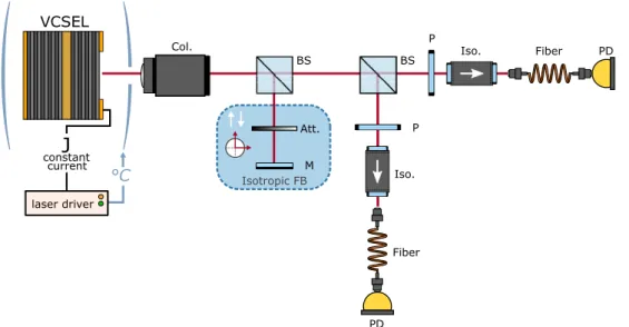
2.3.1 Experimental setup . . . 59
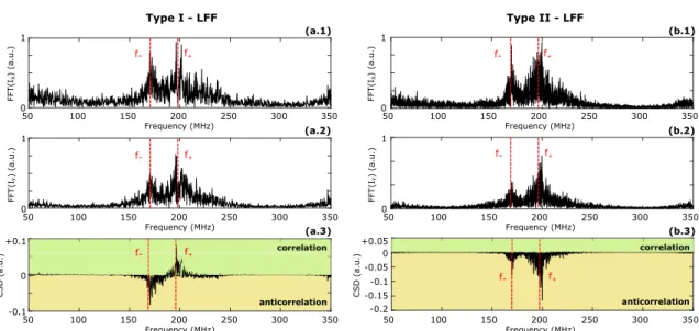
2.3.2 LFF : Double peak and correlation features in the RF spectrum 61 2.4 Physical origin of the double-peak structure . . . 64
2.4.1 Phase-space dynamic and mode/antimode interaction . . . 65
2.4.2 Double-peak structure with a single-mode model . . . 69
2.5 Conclusion . . . 70
3 Vectorial Rogue Wave in VCSEL light polarizations 73 3.1 Observations of Rogue Wave . . . 74
3.1.1 Freak wave in oceanography . . . 74
3.1.2 Identification of rogue waves . . . 75
3.1.3 Rogue Waves in optics and motivation . . . 77
3.2.1 Two types of extreme events in VCSELs . . . 81
3.3 Extreme events statistics . . . 84
3.3.1 Deviation from a Gaussian distribution . . . 84
3.3.2 Waiting times between successive events . . . 85
3.4 Generation rate of extreme events . . . 87
3.4.1 Vectorial Extreme events . . . 89
3.4.2 Noise effect on the generation rate of EEs . . . 90
3.4.3 Differences between Type-I and Type-II LFF . . . 91
3.5 Modal competition effect on the EEs generation rate . . . 93
3.6 Conclusion and perspective . . . 95
4 Sustained oscillations accompanying polarization switching in a laser diode 97 4.1 Square-wave modulation in optics . . . 98
4.2 Bifurcation to high-frequency oscillation in square-wave regime . . . 102
4.2.1 Description of the experimental setup . . . 103
4.2.2 An overview on the observed dynamics . . . 104
4.2.3 Effects of the feedback ratio and the injection current . . . 105
4.2.4 Influence of the delay . . . 106
4.3 Numerical Investigation . . . 108
4.3.1 Rate equations for EEL subjected to a PROF . . . 108
4.3.2 Bifurcation scenario leading to sustained oscillations . . . 109
4.3.3 Influence to the delay . . . 111
4.3.4 Effect of the laser parameters . . . 113
4.3.4.1 Pump parameter P . . . 113
4.3.4.2 Carrier to photon lifetime ratio T . . . 115
4.3.4.3 Linewidth enhancement factorα . . . 117
4.3.4.4 Gain coefficient ratio k and TM additional lossesβ . 118 4.3.5 Effect of noise . . . 119
4.4 Analytical investigation on the sustained oscillations frequency . . . 122
4.4.1 Steady states . . . 123
4.4.2 Hopf bifurcations . . . 124
4.4.3 Approximations . . . 125
5 Optical chimera in light polarization 129
5.1 Chimera state : a coexistence of coherence and incoherence . . . 130
5.1.1 Demonstration of spatially extended chimera states . . . 131
5.1.1.1 Chemical oscillators . . . 131
5.1.1.2 Optolectronic oscillators . . . 132
5.1.1.3 Mechanical oscillators . . . 133
5.1.2 Chimera states in optical spectrum and virtual-space . . . 134
5.1.2.1 In the optical spectrum of a mode-locked laser . . . . 135
5.1.2.2 In a virtual space from a time-delay system . . . 135
5.1.3 Discussion on optical chimera state . . . 138
5.2 Chimera state in laser polarization . . . 140
5.2.1 Experimental setup . . . 140
5.2.2 Theoretical model . . . 142
5.2.3 Observation of virtual chimera states . . . 142
5.2.4 Stabilization of multi-headed chimeras with a 2nd delay . . . . 144
5.2.5 Multi-stability and chimera-heads mechanisms . . . 147
5.2.6 Influence of the initialization and of the feedback strength . . 149
5.2.6.1 Influence of the initialization . . . 149
5.2.6.2 Influence of the PROF strength . . . 150
5.3 Conclusion . . . 154
6 Conclusion 157 6.1 Summary, contributions and perspectives . . . 157
7 Résumé de la thèse 167
C
H A P1
I
NTRODUCTION
M
ore than fifty years after their invention, lasers keep improving their performances; and their application domains are constantly broadening [1]. It has become a fundamental tool in various fields of metrology as in telemetry to measure distances, for gyroscopes to measure angular speeds, for lidar to detect objects, their motions and even sometime their shapes. In the latter case, it also allows the detection of pollution in air and the measurement of the Earth’s surface topology. Lasers have also paved the way for safer, more precise and/or new treatments in medicine as for the cure of glaucomas which can cause vision losses, to burn cancerous tumors, and even in plastic surgery for long-term hair removal and cellulite erasing. It is also a powerful tool in industry for welding and cutting materials, in telecommunication with the development of fiber optics, in chemistry for spectroscopy and astronomy for the exploration of cosmological physics.The goal of this introduction is to present the context of this thesis and to provide the required basics to follow the thesis work. It is also an opportunity to acknowledge the work of great scientists that laid the foundation for laser modern applications such as Charles H. Townes, inventor of the maser, pioneer of the laser who persevered through thick and thin in his research.
This Chapter is organized as follows : first we introduce the story of laser as it was related by Townes in his autobiography published in 1999 [2]. Then, we explain what
a laser is and its principle of operation. We also provide details on the well-spread semiconductor lasers. Secondly, we highlight the discovery of chaos and nonlinear dynamics and how lasers are able to display such dynamics. We emphasize on the importance of chaotic lasers in many innovative applications. Finally, we introduce the main objectives of our work and summarize the outlines of the thesis.
1.1
From maser to laser : the story of Charles H.
Townes
The goal of this section is to recall the work of Charles H. Townes (1915-2015), inventor of the maser1 and Nobel Laureate in 1964. In his book How the Laser Happened published in 1999 [2], Townes relates about his adventure that led him to design the first maser despite the criticisms of famous physicists.
In 1935, Townes was one of the only two students in physics from Furman University. He was offered an assistantship at Duke University, where he worked on Van de Graff generators, an accelerator of protons using static electricity. At that time, he failed to get a full-time fellowship in several other universities better known for their physics programs. Nevertheless, with hindsight, he will later be always grateful for those failures as he decided afterward to go to Caltech without any financial support in 1937. His PhD thesis was on the separation of stable isotopes of oxygen, nitrogen and carbon upon which he improved his spectroscopy skills. This later served him as a starting point for the realization of the first maser. In 1939, he got a position at AT&T’s Bell Labs and quickly worked on military radar bombing systems as the United States were about to get involved in the World War II. The purpose of his work was probably aimed to be used for the atomic bomb just after the discovery of nuclear fission. One of the challenge he faced was to reach a sub-centimeter aiming-accuracy that would be achieved by generating an electromagnetic wave at the same order of wavelength. He did extensive study of ammonia (NH3), a
highly present molecule in the Pacific showing strong resonances at sub-centimeter wavelength. The war ended and Townes never reached such accuracy. However, his research on ammonia absorption led him to pursue in sub-centimeter wavelength
generation from molecular spectroscopy. In 1950, he was invited to join Columbia University by Isidor Isaac Rabi, who received the Nobel prize in physics in 1944.
In 1951, a small committee of physicists including Townes gathered to find a proper way to generate sub-centimeter wavelength. It was already known at that time that molecular transitions involve absorption and emissions at millimeter-wavelength. However, in order to get an output energy sufficiently high, the sample had to be shined by a tremendous amount of power. The meeting ended without any convincing solution. However, it was during this meeting that Townes thought about making a cavity in which excited molecules would be placed. From the stimulated emission theory of Einstein, the electromagnetic wave would be amplified after crossing the sample of molecules [see Fig. 1.1]. He kept the idea for himself as he wasn’t that sure yet how far it would go.
Figure 1.1: First draft of a maser drawn by Townes during the sub-centimeter committee meeting in 1951. It consists on a constant beam of excited molecules sent into a cavity. The figure is taken from Ref. [2].
Back to Columbia University, he double-checked his first calculations based on ammonia as the excited medium. He predicted not only an amplification of the wave, but also a coherent beam at nearly a constant wavelength. With Jim Gordon, a freshly graduated student from MIT and Herb Zeiger, a former PhD student of Isaac Rabi in the field of molecular beam, Townes launched his first experimental
project on maser. For this first attempt, they settled on using the strongest ammonia transition at 1.25 cm. Two years after the beginning of the project, the maser was still not running and Townes an its coworkers faced a lot of criticism from Rabi and Kusch2. As reported by Townes in his book, he was told : "you should stop the work you are doing. It isn’t going to work. You know it’s not going to work. We know it’s not going to work. You’re wasting money. Just stop!".
Three months later, after carefully trying different angles for the gaz beam and looking for the good material for the cavity to lower the losses, Jim Gordon has achieved the first working maser. It was in April of 1954. The same day, they decided to name this device maser which stands for "microwave amplification by stimulated emission of radiation" [3, 4]. The picture in Fig. 1.2 shows J. Gordon and C.H. Townes with another maser build after the prototype. This second maser was build to measure the maser spectral purity by making both masers beating together.
Figure 1.2: J. Gordon (right) and C.H. Townes (left) with the second maser at Columbia University.
With this demonstration, masers have aroused interest of many groups in spec-troscopy and atomic clocks. Some have even stated maliciously that maser stood for "means of acquiring support for expensive research" and indeed it did give Townes research support. However, still this maser wasn’t of great use as it wasn’t tunable in wavelength and wasn’t neither at sub-centimeter wavelength.
In 1958, with Schawlow, one of this his former post-doc and actual brother-in-law, he published one of the most important paper for the future design of optical maser i.e. laser which stands for "Light amplification by stimulated emission of radiation" [5]. They theoretically considered a Fabry-Perot cavity and explained how the cavity selects resonant wavelengths while suppressing the others. It was in 1960, that Theodore Maiman demonstrated for the first time a working laser [6] using a ruby crystal and two layers of aluminum forming the aforementionned Fabry-Perot cavity. The next year, Ali Javan, a former PhD student of Townes, demonstrated the helium-neon laser [7]. In 1962, Robert N. Hall [8] demonstrated the first semiconductor laser.
Figure 1.3: (left to right) Theodore Maiman, Ali Javan and Robert N. Hall
Charles H. Townes received in 1964 the Nobel Prize in physics3 for the invention of maser that paved the way for lasers. Since then, lasers have been used in numerous fields of research, leading to important Nobel Prize discoveries : D. Gabor in 1971 for holography, N. Bloembergen, A. Schawlow, K.M. Siegbahn in 1981 for laser spectroscopy, S. Chu, C. Cohen Tannoudji, W.D. Phillips in 1997 for atom cooling 3that he shared with Bassov and Prokhorov, two Russians that independently worked also on
using laser, and B.C. Barish, Rainer Weiss, K. Thorne in 2017 for laser interferometry technique used in the LIGO detector and for the observation of gravitational waves.
1.2
Physics of lasers
The underlying theory of maser, described in the previous section, has later inspired the invention of laser. In this section, we will explain the main aspects of this theory and introduce semiconductor laser.
1.2.1
Principle
Laser is an acronym which stands for light amplification by stimulated emission of radiation. The mechanism of stimulated emission was predicted in 1916 by Albert Einstein [9] from quantum theory [10]. Stimulated emission provides a second coherent photon with the similar energy than the incoming photon, hence it creates a coherent amplification of the light. The energy of a photon Ephot is given by Ephot=
hν with h the Plank constant and ν the electromagnetic frequency of the photon. However, stimulated emission also competes with other light-matter processes : the spontaneous emission and the absorption. In Fig. 1.4, we describe these mechanisms and consider a single atom with two atomic levels : E1and E2which are respectively
the ground-state and the excited-state (i.e. E2> E1). The three mechanisms are
described as follow :
• Absorption [Fig. 1.4 (a)] : an incoming photon is absorbed by an atom in the energy level E1. The atom goes to the excited energy level E2
• Spontaneous emission [Fig. 1.4 (b)] : the atom is already in its excited energy level E2. Without any external perturbation, the atom spontaneously goes down
to the ground state E1by emitting a photon of energy Ephot= E2− E1. Here
the photon has a random phase.
• Stimulated emission [Fig. 1.4 (c)] : the atom is already in its excited energy level E2. An incoming photon of energy Ephot= E2− E1 stimulates the
transi-tion of the atom toward the ground state E1. The process is accompanied by
the emission of an additional photon with identical phase and frequency to the incoming photon : it brings light amplification.
Photon Photon Photon Photon
(a) (b) (c)
E1
E2
Figure 1.4: Light-matter mechanisms in a two-energy level system with E1 the
energy of the ground state and E2 the energy of the excited state (a) Absorption
of a photon by an atom in its ground state E1 causing its transition to the excited
state E2. (b) Spontaneous emission of a photon by an atom in its excited state E2
causing its transition to the ground state E1. (c) Stimulated emission by an atom in
its excited state E2due to the stimulation of an incoming photon. The transition of
the atom toward the ground-state E1creates a second identical photon.
Hence, when stimulated emission becomes the dominant process, light amplifica-tion is obtained. However, it requires to have more atoms in the excited state than in the ground state. This situation is called population inversion. It can be obtained with different methods called pumping. For the gas maser of Townes [3], population inversion was achieved by continuously injecting excited molecule of ammonia. For the ruby laser of Maiman [6], the pumping is achieved from a light source that cause absorption. For the Helium-Neon [7] and the semiconductor laser [8], the pumping is achieved by applying an electrical current to the active medium.
Finally, wavelength selection is performed by placing the gain medium inside a resonant optical cavity. Traditionally, the resonator is a simple Fabry-Perot cavity made of parallel and partially reflecting mirrors. Only electromagnetic waves which satisfy the boundary conditions imposed by the mirrors can constructively propagate back and forth in the cavity. They are called modes of the laser and their optical frequency difference∆f is given by the Free-Spectral Range (FSR) :
(1.1) ∆f = FSR = c
2L,
with c = 299792458 m/s the speed of light and L the length of the Fabry-Perot cavity. Furthermore, only modes that have an energy, hence an wavelength, that matches the difference of energy between the ground-state and the excited-state of the active medium can be amplified. The cavity also reduces the amount a pumping necessary
to achieve population inversion as it ensures a large number of photons in the gain medium which participate in the stimulated-emission process.
The laser starts to emit a coherent beam of photons when the gain in the cavity exceeds the losses (caused by absorption and by photons exiting the cavity). This particular state, where the gain equalizes the losses, is called the laser threshold. Figure 1.5 shows a typical instance of light-pump curve of a laser. When the pump energy is too low to compensate the losses in the cavity, the laser emission is mostly driven by the spontaneous emission. On the contrary after the threshold, population inversion is reached, the stimulated emission becomes the dominant process and coherent emission of light is obtained.
In summary, lasing effect requires three main ingredients: • A gain medium with stimulated emission (i.e. amplification), • A pump to ensure population inversion,
• A resonator to select the emission wavelength and to reduce the amount of pumping necessary for lasing.
Laser threshold
spontaneous emission stimulated emission
Optica
l P
ower
Pump parameter
Figure 1.5: Illustration of a typical light-pump curve of a laser. Before the threshold, the laser emission is mostly driven by spontaneous emission of incoherent light. At the threshold, the gain equalizes the losses in the laser cavity. A coherent light is obtained beyond the threshold point where stimulated emission becomes the dominant radiative process.
1.2.2
Semiconductor lasers
Semiconductor laser (or laser diode) is today one of the most common type of lasers. Due to their small size, they are mass-produced at a very low-cost. Here, we introduce their basic structure and mechanism.
In semiconductor lasers, radiative transitions typically occur between upper energy states in the conduction band and lower energy states in the valence band. Conduction and valence bands are separated by an energy band-gap where electrons are forbidden. At zero temperature, electrons occupy energy states in the valence band. On the contrary, when increasing the temperature, some of the electrons might occupy energy states in the conduction band leaving an empty space in the valence band called holes that can be considered as a virtual positively charged particle.
In addition, as seen previously, population inversion is a vital condition to obtain optical amplification. The simplest semiconductor structure to achieve population inversion in the so called p-n junction in which a p-type semiconductor is in contact with a n-type semiconductor. p- and n-type semiconductors are defined by their doping i.e. the addition of impurities in the material. In p-type semiconductor, the doping creates an excess of holes while in n-type, it creates an excess of electrons.
P N + V - electrons holes population inversion conduction band valence band (a) (b) N P
Figure 1.6: (a) Illustration of a p-n junction with a forward bias V. (b) Corresponding energy band diagram. Population inversion is achieved at the junction.
When these two semiconductors are in contact, diffusion of carriers occurs : the electrons diffuse toward the p-region and the holes toward the n-region. The diffusion stops when an equilibrium is reached. This effect creates a difference of potential at the junction which acts as barrier of potential preventing any further electrons to flow toward the p-region and holes toward the n-region. The barrier can be lowered by applying a forward bias between the p-region and the n-region allowing the
electrons in the n-region to drift toward the p-region and the hole in the p-region to drift toward the n-region. This constant stream of carriers creates a tiny region at the junction where population inversion is observed as depicted in Fig. 1.6. A p-n junction is also referred to as a homojunction because the band gap is similar in both the p and n-regions.
Although laser action can be obtained from an homojunction, it has soon been found to be unsatisfactory as it requires low temperature, high pumping current and it was difficult to maintain a continuous-wave operation [11]. In 1963, Herbet Kroemer, Nobel Laureate in 2000, proposed another structure where a small band gap material is placed in between two higher band gap materials. This structure is called double heterostructure [12]. In Fig. 1.7, we show a typical double heterostructure. The double barrier surrounding the active region (p-region here) prevents the electrons to flow toward the p+-region and the holes toward the n+-region. This greatly reduces the threshold current as it leads to a better carrier confinement. In addition, it provides a waveguide-like structure as the cladding layers have usually a smaller refractive index than the active layer. Hence, this structure also improves the gain uniformity along the direction of propagation in the active medium and enhances the stimulated emission process.
Photon conduction band valence band N+ P P+ electrons holes (a) (b) population inversion N+ P P+ + V
-Figure 1.7: (a) Illustration of a double heterostructure made of two p-n junctions. (b) Corresponding energy band diagram. Population inversion is achieved in between the two p-n junctions.
1.2.3
From edge to surface-emitting lasers
Historically, the Edge-emitting laser (EEL) in Fig. 1.8 (a) is the original structure proposed for semiconductor lasers [12]. It’s energy-band diagram rely on the dou-ble heterostructure shown in Fig. 1.7. The resonator length is typically about few hundreds of micrometer to one millimeter which is sufficient to achieve high-gain without the need of high-quality Fabry-Perot mirrors. In fact, the resonator is simply based on Fresnel reflections at the air/semiconductor interfaces (with usually a power reflectivity of ≈ 30%). The light is emitted from the edge of the device i.e. orthogonal to the semiconductor growth direction. In addition, due to the geometry of the active region, EEL shows a larger region of amplification in the x-direction than in the y-direction. As a result, the polarization of the output light is usually polarized linearly in the x-direction called the TE-mode while the TM-mode polarized in the y-direction is depressed. Active Medium Active Medium Surface DBR Bottom DBR (a) (b) Semiconduct or gro wth direc tion y z x
Figure 1.8: Illustration of (a) an EEL emitting a laser beam orthogonally to the semiconductor growth direction and (b) a VCSEL having the active medium in between two DBR. The light is pointed in the same direction as the semiconductor growth direction.
However, one main drawback of EEL is that, due to their direction of emission, one cannot test the laser directly on the wafer or neither making a 2D-array of it without cleaving it first. In 1979, Soda et al. proposed a double-heterostructure which allows the emission of a 1.2 µm light in the semiconductor-growth direction : the vertical-cavity surface-emitting laser (VCSEL) [13]. In addition, contrary to EELs which typically have a cavity length of the order of micrometers, the VCSEL cavity length is usually of the order of nanometers. As a result, to keep a reasonable threshold
current value, one has to decrease the losses, hence increasing the mirror reflectivity dramatically. In the first VCSEL proposed, the mirrors were made from gold [14]. However, although gold has almost a reflectivity of 95% at 1.2 µm wavelength, the device still requires a tremendous amount of pumping current with a threshold at 900 mA (11kA/cm2). The need of high-reflectivity mirrors has led to the use of distributed Bragg reflectors in which different layers of semiconductor with alternatively low and high refractive indices are stacked vertically. The first proposal was made by Ogura et al. in 1987 [15] following by a great improvement in term of reflectivity (in the order of 99%). This has allowed a threshold current of about 1 mA in 1989 by Jewell et al. [16].
In addition of its capability to emit light from the surface, VCSEL demonstrates nowadays very low threshold current (≈ 0.5 mA) and emits a quasi-perfect circular beam due its cylindric structure compared to EELs which usually emits elliptical beam. Furthermore, as we will discussed in Chapter 2 VCSELs show intriguing polarization properties which are detrimental for telecommunication applications but might also bring interesting dynamical behaviors. Indeed, contrary to EEL, the geometry of the active region in VCSEL does not favor any polarization direction resulting in polarization instabilities [17, 18].
1.2.4
Relaxation oscillations
As we have seen, laser operation relies on the interplay between photons and carriers, which is at the origin of what is called relaxation oscillations. For example, an increase of the pumping current leads to an enhancement of the population inversion in the active medium. Thus, as more electrons are exited, the stimulated emission rate increases creating more photons in the cavity and enhancing the optical power. However, while stimulated emission processes occur, more and more carriers are consumed. The decrease in carrier weakens the stimulated emission rate leading to lower optical power until the carriers build up again. The loop occurs periodically several times and manifests itself by damped oscillations of the laser output power until the laser settles on his new operating point. This dynamic is referred to as relaxation oscillations. The corresponding frequency is usually of the order of 1 to 15 GHz in semiconductor lasers.
0 0.5 1 1.5 0.4 0.6 0.8 Time (ns) Otica l output po wer (a .u.) Pumping current (a.u.) 0 1 TRO=1/fRO (a) (b)
Figure 1.9: (a) Step in pumping current occurring at t=0. (b) Before the step, the laser is operating in a continuous wave emission. A t=0, the pumping current is increased resulting a relaxation oscillations of the output power at a frequency fRO≈ 11 GHz.
The oscillations amplitude decreases until reaching another steady-state with higher optical power.
The law that drives the relaxation oscillation frequency fRO to the pumping
current J is given by : (1.2) fRO=1 2 s 1 τcτp ( J Jth− 1) ,
where τc is the carrier lifetime,τp is the photon lifetime and Jthis the
pump-ing current at the laser threshold. The relaxation oscillation frequency is in the same range that the direct modulation frequency limit i.e. the maximum frequency achieved by a modulation of the pumping current.
Experimentally, fROcan be deduced by applying a step of current as described
in Fig. 1.9 or by measuring the relative intensity noise (RIN) of the laser. The RIN describes the temporal fluctuation of the laser output power when operating at constant parameters (fixed current and temperature). It is usually visualized in the Radio-Frequency (RF) domain and is characterized by a peak at the relaxation oscillation frequency fRO. When measuring the RIN of a laser on a RF spectrum
signal Nmeas [19]. Neq is mainly driven by the thermal noise Nth which can be
measured before switching on the laser. For a more accurate measure of RIN, the shot-noise Nsn of the photodiode has to be also measured. Shot-noise originates from
random excitations of carriers in the photodiode which depends on the mean optical intensity that reaches the detector.
1.3
Some Applications of lasers
In the previous sections, we have related the story that led to the invention of lasers and their fundamental physics. In the following, we have selected two applications of lasers which have revolutionized modern society such as optical telecommunication, and optical ranging. Of course, there would be many additionnal laser applications to cite, and more details can be found in many books [1, 14, 20].
1.3.1
Optical communications
The rise of modern optical communications is related to the invention of four main components : semiconductor lasers, low-loss optical fibers [21], optical amplifiers [22] and photodetectors as shown in Fig. 1.10.
Semiconductor Laser
Optical
Amplifier AmplifierOptical
Optical fiber Optical fiber Optical fiber
Photodetector
150 - 200km
DFB - Laser EDFA Single-mode
silica fiber
PN junction
Figure 1.10: Illustration of modern optical communication architecture. A semicon-ductor laser emits a modulated light into an optical fiber. Each 150 − 200km an optical amplifier amplifies the optical signal until reaching a photodetector.
Back to basics, modern communications are digital implying that the signal is modulated as function of bits "0" or "1". For example, in optical links, the absence of light defines a "0" and the detection of light a "1"4. Nowadays, optical signals can
achieved data rate about 2.5 Gb/s to 40 Gb/s; this means light is modulated in this range of frequency. As a comparison, the first Internet system based on electrical links could only transmit data at 56kb/s ! The advantages of semiconductor lasers are threefold : 1/ they have low energy consumption and high optical power, 2/ the optical linewidth is narrow which allows multiplexing at hundred of wavelengths in a single fiber, 3/ they support high modulation speeds. In the latter case, lasers are limited to ≈ 10 GHz and external modulators are used to increase the modulation speed. Indeed, as we will see later, a modulation frequency of the pumping current close to the relaxation oscillation frequency may induce unwanted erratic fluctuations.
The second main discovery that led to optical communication was the optical fiber technology. Charles K. Kao received the physics Nobel Prize in 2009 for this discovery. The most widespread silica fiber has only an attenuation of 0.2dB/km at wavelength close to 1.5µm (also called the conventional band or C-band). Although the signal power is divided by a factor two after 15 km, propagation over 150 to 200 km is easily achieved. As a comparison, at this range of modulation frequency, electrical signal would be completely lost after hundreds of meters. The transverse profile of the fiber is also crucial : a single mode fiber (with a core diameter < 8 µm) is mandatory to minimize temporal deformation of the optical signal. Nonetheless, very lately, multi spatial modes multiplexing in multimode fibers [23] are under investigation in order to increase the data rate in optical telecommunication. A new world record of 10 Pb/s in a single fiber has been achieved with this technique [24] in 2017.
After 150 km of propagation in fibers, an optical amplifier is placed. The un-derlying physics behind amplifiers also rely on stimulated emission of light. The most common technology is the Erbium-Doped Fiber Amplifier (EDFA) [22] that can directly amplify the light inside a doped fiber. Usually, the amplifier is pumped by a 980 nm laser. Finally, the light is detected by a semiconductor photodetector whose physics are very similar to semiconductor lasers. Instead of stimulated emissions at its PN junction, photodetectors create pairs of electrons and holes from absorption of light hence modifying the voltage at the junction.
1.3.2
LIDAR for optical ranging and aerosol detection
LIDAR stands for light detection and ranging. Similarly to RADARs, LIDAR are used for ranging applications but using light instead of microwaves. For LIDARs, a
laser emits pulses at nanosecond scales. When the light encounters an obstacle, a part of it is reflected back to the LIDAR. The position of the obstacle is deduced by measuring the delay between the emission and the detection time.
It is also possible to measure the speed of the obstacle using the Doppler effect. To do so, their are two mains techniques : either measuring the deformation of the pulse shape by a moving object or by measuring the optical frequency shift of the light. The latter technique is called heterodyne detection.
LIDAR technology is used in a variety of field such as for measuring the wind direction map and amplitude for wind farms, for the detection of threats in military context, for the detection of obstacle for future autonomous cars, drones and robots, for elevation measurement, for speed measurement of cars by police officers etc. Lately, an impressive technique has been reported for the detection of hidden object [25] relying of the measurement of photons scattered by several objects in the environment. They used a femtosecond pulsed laser in order to achieve better signal-to-noise ratio on their detector.
1.4
Nonlinear dynamics and chaos in laser diodes
Dynamical system can be found in a large variety of subjects going from physics to biology, chemistry and engineering [26]. It has first started in the 17th century when Newton found the differential equations for the laws of motions and objects gravitational interactions such as gravitational motion of planets. Following the Kepler’s empirical laws, he solved the two-body problem taking the example of the earth trajectory around the Sun. However, physics have struggled for decades on the three-body problem when adding for example the moon dynamics into the equations. In the 19th, Poincaré demonstrated that this problem doesn’t have an explicit solution i.e. one cannot find an explicit set of formulas that gives the positions of the moon, sun and earth simultaneously. This discovery by Poincaré is often considered as the first step towards what is called today nonlinear dynamics, i.e. a dynamical motion that does not directly and linearly relate to the changes in their operating conditions. However, due to the complexity of such systems, Poincaré’s works have encountered only a little impact in the scientific community until the 50’s with the invention of computers. It was in 1963 that Edouard Lorenz demonstrated from numerical
simulations that a set of deterministic equations5 describing a simple model of the atmosphere may result in a complex trajectory [27] : more specifically, an aperiodic dynamic that never repeats itself and that shows an utmost sensitivity to initial conditions. Such a dynamics has later been referred to as chaos [28].
In 1975, Haken showed theoretically the close analogy between laser equations and those used by Lorenz [29]. In this section, we will first introduced the work of Lorenz and the basics of chaotic dynamics and develop its analogy with lasers.
1.4.1
The strange-attractor of Lorenz
In 1963, while investigating convective fluids for weather prediction, Lorenz showed that a nonlinear system described by three state-variables shows large regions of parameters where the solutions never settle down on a periodic state or an equilibrium state. It was the first demonstration of chaos. The model he used is given by a set of three simple equations [27] :
d X dt = −σX + σY , (1.3) dY dt = −X Z + rX − Y , (1.4) dZ dt = X Y − βZ, (1.5)
where σ, r and β are the parameters of the system and X, Y and Z the state variables. As an example, we show in Fig. 1.11 (a-c) the time evolution of the state variables when taking the parametersσ = 10, r = 30 and β = 8/3. All three variables shows an erratic behavior despite no randomness (such as noise) is introduced in the equations. In Fig. 1.11, we show the trajectory of the system in the phase space where each axis stands for one state variable. The trajectory consists on two wings centered around two fixed points. In this dynamic, the system remains confined around what has been called a strange attractor as it bounds all trajectories in its neighborhood.
-20 0 20 X -50 0 50 Y 0 500 1000 1500 2000 2500 3000 3500 4000 4500 5000 Time (a.u.) 0 20 40 Z 0 40 10 20 30 Z 40 20 Y 50 X 10 -15 -40 -20 (a) (b) (c)
Figure 1.11: Time-evolution of the state variables (a) X, (b) Y and (c) Z and (d) the corresponding trajectory in the phase space. The simulated parameters areσ = 10, r = 30 and β = 8/3.
This attractor was also referred to as the Butterfly of Lorenz for its comparison to a butterfly and that has given the expression : the butterfly effect. The butterfly effect is a metaphor in chaos theory illustrating the sensitivity on initial conditions. Indeed, two nearby trajectories of a chaotic system diverge from each other exponentially fast. We illustrate this sensitivity in Fig. 1.12 (a) where we show the time evolutions of the variable X for two different sets of initial conditions [X0, Y0, Z0] while keeping
the parameters fixed. In blue, we have initialized with [0, 1, 1.05] while in orange we have chosen a different but yet very close set [0.000001, 1.000001, 1.05000001]. At the beginning, both time series remain quasi-identical until t > 5000 where differences appear. This is confirm in Fig. 1.12 (b), where the Euclidean distance6 between the two attractors is shown. At first, both trajectories are following the same journey until their distance increases quickly around t = 5000. However, they remain confined relatively close to each other as they are both attracted towards the same attractors.
0 5000 10000 15000 -20 0 20 0 5000 10000 15000 0 20 40 60 Time (a.u.) (a) (b) X Eucli dian di stance
Figure 1.12: (a) Time evolution of the variable X for two different ini-tializations. In blue, [X0, Y0, Z0] = [0,1,1.05] and in orange, [X0, Y0, Z0] =
[0.000001, 1.000001, 1.05000001]. (b) Corresponding Euclidean distance between the blue and the orange attractor.
In summary, a chaotic system can be described by the following three criteria : • Aperiodicity : the trajectory does not settle on a steady state nor into periodic
or quasi-periodic orbit as time goes to infinite.
• Determinism : the equations that model the system do not include any random term. Complex dynamics arise from the intrinsic nonlinearity.
• Sensitivity to initial conditions : for two very close initial states, their trajecto-ries diverge exponentially fast.
1.4.2
Bifurcation diagram of the Lorenz’s equations
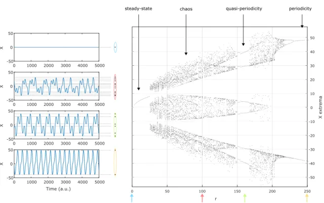
Although chaotic dynamics is easily found from direct simulations of Eqs. (1.3)-(1.5), many different dynamics and complex waveforms can also be obtained when varying the simulation parameters. We show in Fig. 1.13 different solutions obtained when varying the parameter r. For r = 0 in Fig. 1.13 (a), the system is in its quiescent state with no fluctuation of its variables. Increasing r in Fig. 1.13 (b), chaotic fluctuation in observed. For r = 160 in Fig. 1.13 (c), X oscillates quasi-periodically at two different
frequencies and finally for high values of r in Fig. 1.13 (d), a periodic train of pulses is observed. 0 500 1000 1500 2000 2500 3000 3500 4000 4500 5000 -50 0 50 0 500 1000 1500 2000 2500 3000 3500 4000 4500 5000 -50 0 50 0 500 1000 1500 2000 2500 3000 3500 4000 4500 5000 -50 0 50 0 500 1000 1500 2000 2500 3000 3500 4000 4500 5000 Time (a.u.) -50 0 50 X X X X (a) (b) (c) (d)
Figure 1.13: Time evolution of the variable X in the Lorenz equations for (a) r = 0, (b) r = 100, (c) r = 160 and (d) r = 250. Other parameters are identical to those used in Fig. 1.11
In order to have a more comprehensive snapshot of the different dynamics ex-hibited by the system, one convenient tools is the bifurcation diagram. It displays for each value of the parameter r, all the minimum and maximum values (hence extrema values) taken by one state variable. In addition, as we have seen in Fig. 1.13, the qualitative dynamic of the Lorenz’s equations can change as the parameter r evolves. These modifications are called bifurcations and the range of stability of the outcome dynamic is suggested by the analysis of the bifurcation diagram in Fig. 1.14. Although it does not give any information on the waveform of the resulting dynamic, the different dynamical regimes are easily deduced : for r < 25, only one point is displayed per value of r : this is a steady-state; for 25 < r < 150 and 168 < r < 219 there is a large number of points, sign of chaotic behavior, for 150 < r < 168 and 29 < r < 230, X oscillates quasi-periodically with 6 values of extrema and finally for r > 230, X oscillates periodically with only 2 extrema.
0 50 100 150 200 250 -50 -40 -30 -20 -10 0 10 20 30 40 50 0 1000 2000 3000 4000 5000 -50 0 50 0 1000 2000 3000 4000 5000 -50 0 50 0 1000 2000 3000 4000 5000 -50 0 50 0 1000 2000 3000 4000 5000 Time (a.u.) -50 0 50 X X X X r X extrema
steady-state chaos quasi-periodicity periodicity
Figure 1.14: Construction of a bifurcation diagram based on the Lorenz’s equations. r is the bifurcation parameter and X the variable of interest. Other parameters are identical to those used in Fig. 1.11
1.4.3
Analogy between lasers and the Lorenz’s system
In 1975, Haken [29] demonstrated mathematically the close analogy between the model of Lorenz in Eqs. (1.3)-(1.5) and the commonly used Maxwell-Block equations that model laser dynamics. By neglecting the diffusion of carrier and the diffraction of the electrical field in the laser cavity, one can show that lasers can be modeled by the following system of equations :
dE
dt = −κ(1 + iθ)E + P, (1.6)
dP
dt = −γ⊥(1 − iθ)P + γ⊥a(1 + iθ
2)N E, (1.7) dN dt = −γe(N − µ) − (EP ∗− E∗P), (1.8)
N the normalized carrier inversion with respect to transparency7,θ the normalized detuning,µ the normalized injection current, γ⊥the dipolar polarization relaxation rate,γethe carrier decay rate from spontaneous emission and non-radiative
recombi-nation, a the differential gain at the laser frequency,κ the field decay rate.
This system of equations can be redefined by introducing the real and imaginary parts of E and P and considering the following variables
E ≡ r γ⊥µ 2κr (Er+ iEi), (1.9) P ≡ r γ⊥µ 2κr (Pr+ iPi), (1.10) N ≡ µ −µ rN, (1.11) r ≡µa κ (1 + θ 2), (1.12) t ≡ tγ⊥, (1.13) σ ≡ κ/γ⊥, (1.14) b ≡ γe/γ⊥, (1.15)
With these changes, the model reads :
dEr dt = −σ(Er− θEi− Pr), (1.16) dEi dt = −σ(Ei− θEr− Pi), (1.17) dPr dt = − − Pr− θPi+ rEr− NEr, (1.18) dPi dt = −Pi+ θPr+ rEi− NEi, (1.19) dN dt = −bN + ErPr+ EiPi, (1.20)
Finally, if we considerer a single longitudinal mode operation for whichθ = 0 and if Ei= P = i = 0 [30, 31], we obtain :
dEr dt = −σ(Er− Pr), (1.21) dPr dt = −Pr+ rEr− NEr, (1.22) dN dt = −bN + ErPr, (1.23)
which are the Lorenz equation described previously in Eqs. (1.3)-(1.5). As a re-sult, lasers might be thought as good candidates for chaotic behavior. Nonetheless, although the above equations are analogous to the Lorenz’s system, chaos is not always achieved by every single lasers. Indeed, the model of Lorenz implicitly sug-gests comparable relaxation time-scale for each variables which implies that each variable contributes to the dynamic of the system. In lasers though, this is not always true and the dipolar polarization variable Prmight, in some cases, be adiabatically
eliminated from the equations. The laser dynamics in that case is a motion in the plane, hence preventing the observation of chaos [28].
1.4.4
Classification of lasers
In Eqs. (1.6)-(1.8), we have taken into consideration different time constants :κ the field decay rate,γ⊥the dipolar polarization relaxation rate andγethe carrier decay
rate which have been included in the parametersσ and β in Eqs. (1.21)-(1.23). The stability of lasers have been classified in three groups depending of these time scales : classe A, B and C [32, 33].
1.4.4.1 Class C lasers
When all the time constantsκ, γ⊥andγeare in the same order, we must considered all
three equations (1.6)-(1.8). As illustrated with the Lorenz’s model, several dynamics including chaos can be obtained. This class encompasses N H3laser [34, 35], Ne-Xe
lasers emitting a 3.51µm [36], and He-Ne lasers emitting at 3.39µm [37, 38]. We show an example of route to chaos made of successive period double of the optical power in Fig. 1.15. It shows the optical spectrum of the measured signal. The different solutions are obtained by tilting one mirror of the Fabry-Perot cavity forming the cavity. While tilting the mirror from it’s ideal position, the output optical power
shows first oscillation at a frequency of 7 MHz followed by successive period doubling (or frequency halving) : a period-2 at 3.5 MHz, a period-4 at 1.75 MHz and a period-8 at 0.875 MHz until it reaches fully developed chaos in Fig. 1.15 (e).
Figure 1.15: Experimentally observation of the optical spectrum of an He-Ne laser emitting a 3.39µm when tilting one Fabry-Perot mirror. (a) Period-1 oscillations, (b) Period-2 oscillations, (c) Period-4 oscillations, (d) Period-8 oscillations, (e) chaos. The figure is taken of Ref. [38]
1.4.4.2 Class B lasers
In class B lasers, the dipolar polarization rateγ⊥is high enough compared toκ and
γethat the equation (1.7) can be adiabatically removed from the system of equations.
As a result, class B laser are only modeled by 2 equations making then intrinsically stable [28]. However, as we will see in the next section, instabilities can be unlocked with class B laser by the addition of external perturbations. Class B lasers encompass semiconductor, CO2 and fiber lasers.
1.4.4.3 Class A lasers
Class A lasers are characterized by their long photons lifetime i.e.κ is very small compared to γ⊥ and γe. Therefore, the equation for the population inversion N
and the dipolar polarization P can be adiabatically eliminated. As a result only the equation for the field E remains. Class A laser are the most stable lasers. It comprises visible He-Ne, Ar-ion and dye lasers.
1.4.5
Unlocking nonlinear dynamics in semiconductor lasers
1.4.5.1 Different approaches
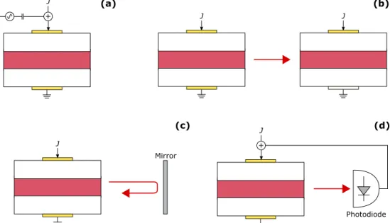
As we have seen, class B lasers are intrinsically stable. During the last 40 years, many techniques have been employed to unlock nonlinear dynamics as it can be useful for various applications (see Section 1.5). In Fig. 1.16, we summarize the main
configurations that allow rich nonlinear dynamics in semiconductor lasers [39]. For all of them, the idea is to increase the number of degrees of freedom of the system from 2 to 3 or even infinite for some cases.
J Mirror J J J + J + Photodiode (a) (b) (c) (d)
Figure 1.16: Different ways to unlock nonlinear dynamics in semiconductor lasers. (a) Direct current modulation, (b) Optical injection, (c) Optical feedback and (d) Opto-electronic feedback.
• Direct modulation in Fig. 1.16 (a): Under certain conditions, direct modu-lation of the laser injection current can induce chaotic pulsing. It requires a modulation frequency of the order of the relaxation oscillation frequency with a relatively high modulation depth [40, 41]. In Ref. [42], the polarization properties of VCSEL have been numerically explored under the influence of direct modulation, and chaos was achieved on a broader range of parameters than found in EELs.
• Optical injection in Fig. 1.16 (b): A laser called master injects its light into the cavity of another laser, the slave. A large variety of dynamic can be unlocked when varying the optical frequency detuning between the master and the slave or by increasing the injected power [43, 44]. Some studies have focused on different polarization states of the injected light : either orthogonal to the naturally emitted light of the slave laser [45] or parallel [46]. In other study,
the master laser is settled on an already chaotic dynamic [47]. Optical injection might also induce the so-called injection locking where the laser emission wavelength locks on the master laser wavelength. Injection locking has been shown to enhance the modulation frequency limit of the slave laser [48]. • Feedback in Fig. 1.16 (c-d) : There are two main configurations of feedback
: the optical feedback and the opto-electronic feedback. In optical feedback experiment, a fraction of the laser light is re-injected in the cavity. In opto-electronic feedback experiment, the emitted light is detected by a photodiode and re-injected in the laser through its injection current. In both cases, the feedback induces a time-delayτ which competes with the internal time-scale of the lasers. However they differs in the sense that opto-electronic feedback is incoherent i.e. it does only influence the carrier population while optical feedback is said to be coherent as it interferes with the electrical field. We will later develop the case of optical feedback.
• It is also worth mentioning that chaos has been also achieved in solitary VC-SELs. In some cases, a nonlinear coupling can occur between two-polarization modes, hence unlocking series of bifurcations when changing the injection cur-rent or the temperature or the strain inside the cavity. This has been reported in a quantum-dots VCSEL [49] where the active region is made of tiny dots of active material or in quantum-well VCSELs subjected to a mechanical strain [50]
1.4.5.2 Optical feedback and route to chaos
Among the above mentioned techniques to unlock nonlinear dynamics in semiconduc-tor lasers, optical feedback is probably the easiest way as it only requires a simple mirror as shown in fig. 1.17. In this configuration, the external mirror (placed at a distance L of the laser) and the output facet of the laser form an external cavity. As discussed above, the round-trip time of the light inside the external cavity induces a delayτ =2Lc that interplays with the internal time scale of the laser i.e. the relaxation oscillation period TRO= 1/ fRO.
Another parameter of importance in external cavity laser is the feedback ratio. It is defined as the ratio between the power of the feedback light and the total output
power of the laser. It can be easily tuned by introducing a variable attenuator in the light path.
J
Mirror
External cavity length L
Figure 1.17: Laser diode subjected to an optical feedback. A mirror is placed at a distance L in front of a laser and reflect a small amount of the light back into the laser.
In 1986, Tkach and Chraplyvy identified five dynamical regimes in external cavity lasers based on qualitative modification of the optical spectrum properties [51]. The transition from one regime to another depends of both the external cavity length (or delay) and the feedback ratio as shown in Fig. 1.18.
• Regime I : At very small feedback levels (less than 0.001%), the laser optical spectrum narrows or broadens depending on the phase of the feedback
• Regime II : Regime II is unlocked when the frequency shift induced by the feedback has multiple solutions also called external cavity modes (ECM). ECMs are stationary solutions whose optical frequency is shifted by n2Lc with n an integer. This regime occurs for a small feedback level (less than 0.01%). Experimentally, the laser hops on these different solutions hence leading to different peaks in the optical spectrum. When looking at the corresponding time traces, the hopping is seen as a fluctuation of the optical power. Each ECM is associated with a certain gain i.e. a certain level of output power. • Regime III : For a very narrow region of feedback ratio (close to 1%), the
optical spectrum narrows for all phases of the feedback (all external cavity lengths). In this regime, the feedback favors one mode over the others.
• Regime IV : For moderate value of feedback (about 1%), sidebands appear on the optical spectrum separated from the emission peak by a frequency equal to
the relaxation oscillation frequency fRO. When looking at the corresponding
time trace, the sideband is seen a undamped oscillations at fRO. As the feedback
is increased, the sidebands broaden leading to coherence collapse i.e. chaotic oscillations that reduce the temporal coherence of the laser.
• Regime V : For high value of feedback (higher than 10%), the external cav-ity acts as an extension of the laser. The laser operates on a single narrow longitudinal mode.
Figure 1.18: Five dynamical regimes of an external cavity laser as function of the distance to reflector L and the feedback ratio. Figure taken from Ref. [51].
Although this classification does not provide an in-depth view on the different dynamics that are unlocked with optical feedback, it summarizes the expected behaviors of such system demonstrating for example the need of high suppression ratio isolator (> 40 dB) to prevent any feedback effect. In particular, it does not
relate to some specific features of external-cavity diode dynamics such as the Low-Frequency Fluctuations [52–54] - that we will investigate in Chapter 2 - or neither the Regular Pulse Packages regime obtained for short external cavity (τ < TRO) [55–57].
Different dynamical behaviors also can be obtained when designing the external cavity by including for example : a) a phase-conjugated mirror known to unlock self-pulsing oscillation of the output power at multiples of the external cavity frequency fEC= 1/τ [58, 59], b) a polarization rotating element such as Faraday-rotator leading to square-wave modulation of the output power [60, 61], c) a wavelength filter such as Fabry-Perrot resonators [62] or grating mirrors [63] which only reflects a narrow window of wavelength favoring one ECM over the others, hence stabilizing the laser. The field of laser diode nonlinear dynamics therefore remains very active considering the numerous configurations that unlock complex dynamics and also considering the development of new laser diodes with new physics.
1.5
Applications of chaos in laser diodes
In Section 1.3, we have introduced two examples of laser applications that have greatly impacted modern society : optical telecommunication and optical ranging. We hereby provide extensions of such technologies when using chaotic oscillations of laser diodes. More examples can be found in Ref. [39].
1.5.1
Chaos for secure communication
As described in Section 1.3.1, lasers are ubiquitous in today telecommunication system. Cisco has predicted to reach by 2021 an annual IP traffic of 3.3 ZB (3.3 trillions of GB) compared to the 1.2 ZB in 2016 with more than 58% of the world population connected to internet [64]. This expansion of telecommunication combined to the democratization of digital money transaction requires safer data transmission. Although the most promising technology is the quantum-key distribution (QKD) with an impressive demonstration in 2017 by the Chinese satellite Micius [65] , chaos-based telecommunication can also improve the data security and can be easily incorporated in actual infrastructure [66].
The chaos-based telecommunication relies on the synchronization of two similar laser diodes through optical injection [67–69], one at the emitter side and the other
one at the receiver side. While the emitter’s laser (master) is forced into chaotic oscillation through e.g. optical feedback, the receiver’s laser (slave) is injected with the light provided by the first one. When both lasers are almost identical and operate in similar conditions (current and temperature), the receiver’s laser can exhibit identical chaotic oscillations compared to the emitter’s. The chaotic signal is used here as a carrier and the message is carefully encoded in the chaotic carrier. Since synchronization occurs between the two chaotic signals (at the emitter and at the receiver), a simple substraction of the chaotic output of the receiver with the input of the receiver (chaos+message) yields the message decoding. In addition, as the synchronization can only be achieved by the use of an identical laser, decryption of the message can be hardly performed by a spy. This experiment has already been conducted in the city of Athens, Greece [66].
1.5.2
Chaotic LIDAR for ranging
LIDAR usage is expected to grow quickly in the next few years in crowded environ-ment such as cities and highways. As a result, the probability for on LIDAR device to detect pulses from other LIDAR (causing failures of detection also called ghost images) also increases. In addition, classic LIDAR are vulnerable to jamming i.e. when someone intentionally shines a LIDAR detector, also causing ghost images.
In order to prevent such issue, randomly-modulated LIDARs have been proposed [70]. It consist on the emission of randomly modulated optical power through an ex-ternal modulator. Then, the position of a target is deduced from the cross-correlation between the emitted and the back-scattered signal. As a result, other sources of light contributed solely to noise. However, this technique still has two drawbacks : first, the electronic of modulation needs to be fast which is then very costly, second, it often relies on a pre-designed sequence of random bits that can be detected and reproduced by a jammer.
By contrast, chaotic lidar (CLIDAR) can overcome such problematic as it doesn’t require fast electronic and chaos is by nature unpredictable [71]. It can be achieved by an optical feedback [71] or from an optical injection [72]. However, improvements of CLIDAR is still required for better energy-efficiency. Indeed, usually, the detection electronic is relatively slow (< 1 GHz) while chaotic laser tends to distribute its energy around the relaxation oscillation frequency (≈ 10 GHz) which results in
energy losses by the equivalent detection low-pass filter. In 2018, Cheng et al. [73] proposed a solution based of an homodyne interference arm that redistributes the energy toward low-frequency regions improving the signal-to-noise ratio by 20dB.
1.6
Conclusion, objectives and outlines
In summary, we have briefly introduced the physics of semiconductor lasers and emphasized two types of structure : the Edge-emitting lasers (EEL) and the Vertical-cavity surface-emitting lasers (VCSEL). These devices have revolutionized our mod-ern society with innovative applications. In addition, we bring to light how laser diodes can exhibit nonlinear dynamics including chaos under external perturbation and how it can be of use for data security and lidar technology.
The work presented here is devoted to the generation of nonlinear dynamics in EEL and VCSEL by mean of optical feedback. More specifically, we bring a focus on the polarizations physics of the emitted light. VCSELs can exhibit nonlinear dynamics simultaneously in two polarization modes when subjected to an isotropic optical feedback [57, 74–76]. On the contrary, EELs show a strongly dominant polarization due to its active medium geometry. As a result, under an isotropic optical feedback, only the dominant polarization is excited. For the depressed polarization to participate in the overall dynamic, some studies have modified the external cavity by adding polarization sensitive components [60, 77–79]. In the following, we will investigate both configurations with VCSEL and EEL and analyze the interplay between the polarization modes. These topics have been selected during my PhD for their fundamental and/or applied interests.
In Chapter 2, we report on the main findings on polarization instabilities in VCSELs. First, we introduce the so-called San Miguel, Feng Monoley (SFM) rate equations which are commonly used to model VCSEL polarizations dynamics. Then, we briefly present the VCSEL physics under isotropic optical feedback and focus and the Low-Frequency Fluctuation (LFF) regime. We analyze both experimentally and numerically polarization correlation properties and highlight an intriguing double-peak structure in the RF spectrum of both polarizations. This latter observation is explained in the manuscript in the framework of the dynamical trajectory in the phase-space around stable ECMs and their unstable counterparts.
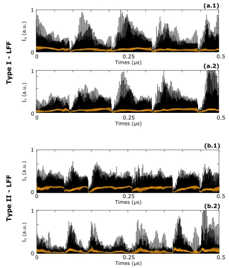
In Chapter 3, we study the generation of high intensity pulses in the total intensity output of VCSEL when operating in LFF regime. Statistics of these pulses show close similarities with the oceanic rogue-waves (RW) which are giant waves emerging on calm seas. We also investigate on the effect of polarization competition on the generation rate of RWs which results in a saturation of the number of RWs when varying the feedback ratio in contrast with the case of single-polarization emission.
In Chapter 4, we investigate the dynamic of EEL subjected to polarization rotated optical feedback (PROF) leading to square-wave (SW) modulation with a periodicity close to twice the external cavity delay. We report on a novel bifurcation resulting in the appearance of fast oscillations on the plateaus of the SW. The experiment and the numerics show that the frequency of these oscillations is neither equal to the external cavity frequency nor to the relaxation oscillation frequency. Analytical study proves that the frequency of those oscillation is proportional to fRO
with a coefficient that depends on the laser parameters, hence can be significantly larger than fRO.
In Chapter 5, we show that our PROF experiment is suitable for the study of asymmetry emerging from spatially extended system such as ring of oscillators. This asymmetry is defined as the coexistence of coherence and incoherence and has been referred to as chimera-state. This is a new paradigm in network systems discovered in 2002 by Kuramoto and Battogtokh [80]. Only few experiments have been able to prove its existence until now but chimera-state is expected to be a generic feature in general physics. From a space-time analogy, we demonstrate that lasers under PROF configuration are able to produce chimera-state with different pattern solutions made of one or several regions of coherence and incoherence called multi-headed chimera.
In Chapter 6, we summarize and conclude on our main findings and discuss about further investigations.
C
H
A
P
2
P
OLARIZATION INSTABILITIES IN
VCSEL
S AND
NON
-
LOCAL CORRELATION PROPERTY IN
LOW
-
FREQUENCY FLUCTUATION REGIME
I
n this chapter, we focus on vertical-cavity surface emitting lasers (VCSEL) . We first introduce the polarization instabilities in VCSEL and explain it phys-ical origin. We also introduce the San Miguel, Feng and Moloney (SFM) rate equations, which consist of a four-level approach to model the polarization behavior of VCSEL. Although polarization instabilities are detrimental for modern telecom-munication systems, we provide here a discussion about their possible interest for future application in communication and information processing.Secondly, we present the basic physics behind VCSEL under isotropic optical feedback and more specifically in the so-called Low-Frequency Fluctuations (LFF) regime. We unveil, both numerically and experimentally, new correlation properties of the polarization modes that couple non-locally two different time-scales of the polarization dynamics. We furthermore investigate the appearance of an intriguing double-peak structure in the vicinity of the external-cavity frequency observed in the RF spectrum of the modes. An exploration of the literature shows that such feature is more generic than expected as it has been observed in different dynamical regimes and laser systems. However, the physical origin remained elusive over almost three
decades.
Finally, we provide a physical interpretation of these particular features and connect them with the trajectory of the system in the vicinity of ruins of stable and unstable external-cavity modes. We perform a detailed study of the parametric influence (pumping current and time delay) and show that our interpretation for the double-peak holds also for EELs with a simple model that only takes into account one polarization mode, a single round-trip in the external-cavity and one longitudinal mode.
This work has been partially reported in the following journal publication : Uy, C. H., Rontani, D., Breuer, S., and Sciamanna, M. (2017). Non-local correla-tions via chaotic itinerancy in VCSEL with optical feedback. Optics express, 25(6), 6914-6923.
2.1
Polarization properties in VCSELs
As discussed in Chapter 1, the VCSEL is considered as one of the most spectacular recent improvement of semiconductor laser technology allowing cheaper growth process and enabling more efficient optical interconnection [81] and parallel infor-mation transmission [82]. For example, in December 2017, Apple, the multinational firm, announced an investment of 390 millions of U.S. dollar in Finisar, one of the largest VCSEL manufacturer worldwide, as VCSEL is rumored to feature the facial recognition technology in the next generations of mobile devices developed by Apple.
"VCSELs power some of the most sophisticated technology we’ve ever developed and we’re thrilled to partner with Finisar over the next several years to push the boundaries of VCSEL technology and the applications they enable."
Jeff Williams, Chief Operating Officer at Apple However, since its first demonstration in 1979 by Soda et al. [13], their polar-ization direction of emission has shown to be very difficult to predict even among VCSELs that are grown in the same wafer [83]. In addition, although the light emis-sion is usually linearly polarized, its direction may also switch with a slight change of the operating parameters [84]. This polarization instability has prevented the use of VCSEL in data transmission technologies, where stable polarization direction is


![Figure 2.16: Spectrogram of the Y-LP mode in the frequency range (a) f ∈ [200 MHz, 400 MHz] as function of the external-cavity delay (b) f ∈ [0 MHz, 70 MHz]](https://thumb-eu.123doks.com/thumbv2/123doknet/14506572.720203/70.892.160.680.245.672/figure-spectrogram-frequency-range-function-external-cavity-delay.webp)