HAL Id: hal-01554834
https://hal.archives-ouvertes.fr/hal-01554834
Submitted on 11 May 2018
HAL is a multi-disciplinary open access
archive for the deposit and dissemination of
sci-entific research documents, whether they are
pub-lished or not. The documents may come from
teaching and research institutions in France or
abroad, or from public or private research centers.
L’archive ouverte pluridisciplinaire HAL, est
destinée au dépôt et à la diffusion de documents
scientifiques de niveau recherche, publiés ou non,
émanant des établissements d’enseignement et de
recherche français ou étrangers, des laboratoires
publics ou privés.
The VIMOS Public Extragalactic Redshift Survey
(VIPERS): PCA-based automatic cleaning and
reconstruction of survey spectra
A. Marchetti, B. Garilli, B.R. Granett, L. Guzzo, A. Iovino, M. Scodeggio, M.
Bolzonella, S. de la Torre, U. Abbas, C. Adami, et al.
To cite this version:
A. Marchetti, B. Garilli, B.R. Granett, L. Guzzo, A. Iovino, et al.. The VIMOS Public Extragalactic
Redshift Survey (VIPERS): PCA-based automatic cleaning and reconstruction of survey spectra.
Astron.Astrophys., 2017, 600, pp.A54. �10.1051/0004-6361/201630249�. �hal-01554834�
December 7, 2016
The VIMOS Public Extragalactic Redshift Survey (VIPERS)
PCA-based automatic cleaning and reconstruction of survey spectra
?A. Marchetti
2, B. Garilli
2, B. R. Granett
2, 3, L. Guzzo
2, 3, A. Iovino
2, M. Scodeggio
2, M. Bolzonella
4, S. de la
Torre
5, U. Abbas
6, C. Adami
5, D. Bottini
2, A. Cappi
4, 7, O. Cucciati
10, 4, I. Davidzon
5, 4, P. Franzetti
2,
A. Fritz
2, J. Krywult
8, V. Le Brun
5, O. Le Fèvre
5, D. Maccagni
2, K. Małek
9, F. Marulli
10, 11, 4,
M. Polletta
2, 12, 13, A. Pollo
9, 14, L.A.M. Tasca
5, R. Tojeiro
15, D. Vergani
16, A. Zanichelli
17, S. Arnouts
5, 18,
J. Bel
19, E. Branchini
20, 21, 22, J. Coupon
23, G. De Lucia
24, O. Ilbert
5, T. Moutard
255, L. Moscardini
10, 11, 4,
and G. Zamorani
4(Affiliations can be found after the references) Received ; accepted
ABSTRACT
Context. Identifying spurious reduction artefacts in galaxy spectra is a challenge for large surveys.
Aims. We present an algorithm for identifying and repairing residual spurious features in sky-subtracted galaxy spectra with application to the VIPERS survey.
Methods. The algorithm uses principal component analysis (PCA) applied to the galaxy spectra in the observed frame to identify sky line residuals imprinted at characteristic wavelengths. We further model the galaxy spectra in the rest-frame using PCA to estimate the most probable continuum in the corrupted spectral regions, which are then repaired.
Results. We apply the method to 90,000 spectra from the VIPERS survey and compare the results with a subset where careful editing was performed by hand. We find that the automatic technique does an extremely good job in reproducing the time-consuming manual cleaning and does it in a uniform and objective manner across a large data sample. The mask data products produced in this work are released together with the VIPERS second public data release (PDR-2).
1. Introduction
Large surveys of galaxy redshifts represent one of the pri-mary means to explore the structure of the Universe and the evolution of galaxies. These include wide-angle surveys at relatively low redshift, notably the SDSS (York et al. 2000) and 2dFGRS (Colless et al. 2001) and deeper, narrower probes including VVDS (Le Fèvre et al. 2005; Garilli et al. 2008), DEEP2 (Newman et al. 2013) and zCOSMOS (Lilly et al. 2009) [see Guzzo et al. (2014) for a more complete re-view of current and past surveys]. The recently completed VIMOS Public Extragalactic Redshift Survey (VIPERS) has built a sample that is at the same time deep, densely sampled and covers a volume similar to the 2dFGRS, but at z = [0.5, 1.2] (Scodeggio et al. 2016; Guzzo et al. 2014; Garilli et al. 2014).
Send offprint requests to: A. Marchetti e-mail: [email protected]
? based on observations collected at the European Southern
Observatory, Cerro Paranal, Chile, using the Very Large Tele-scope under programs 182.A-0886 and partly 070.A-9007. Also based on observations obtained with MegaPrime/MegaCam, a joint project of CFHT and CEA/DAPNIA, at the Canada-France-Hawaii Telescope (CFHT), which is operated by the Na-tional Research Council (NRC) of Canada, the Institut NaNa-tional des Sciences de l’Univers of the Centre National de la Recherche Scientifique (CNRS) of France, and the University of Hawaii. This work is based in part on data products produced at TER-APIX and the Canadian Astronomy Data Centre as part of the Canada-France-Hawaii Telescope Legacy Survey, a collab-orative project of NRC and CNRS. The VIPERS web site is http://www.vipers.inaf.it/.
These surveys provide unique insight into both cosmol-ogy and galaxy formation. The spectra of extragalactic sources can enlighten our understanding of the underlying processes of galaxy evolution through the measurements of physical properties such as star formation, metallicity, gas content and rotational velocity. The observed redshift con-tains not only information on the galaxy distance from the uniform Hubble expansion, but also the imprint of peculiar motions produced by the growth of structure. Statistically, this information can be extracted and used to test the na-ture of gravity (see e.g. the parallel papers by de la Torre et al. 2016; Hawken et al. 2016; Pezzotta et al. 2016; Wilson et al. 2016). Knowledge of precise distances to galaxies also enables us to map the cosmic web and characterize galaxies with respect to the local density field; this is the starting point to study the interplay between galaxy properties and their environment (see the parallel paper by Cucciati et al. 2016).
Spectra obtained from ground–based optical surveys suffer from contamination from signal coming from the Earth’s atmosphere (besides instrumental and data reduc-tion artifacts). This sky emission affects the identifica-tion and measurements of emission and absorpidentifica-tion fea-tures, which are used to determine the redshift; they will also corrupt estimates of line intensities, through which galaxy properties are characterised. These defects can be cured manually, when the number of spectra is small. In large modern surveys, however, automatic data reduction pipelines have become mandatory, as to efficiently manage the large quantity of data (e.g. Stoughton et al. 2002; Garilli et al. 2010, and references therein).
A&A proofs: manuscript no. Masking_paper
Spectroscopic data reduction pipelines perform the sub-traction of sky lines and other known features; however, this operation is not free of errors, depending on various effects such as instrument optical distortions or the presence of fringing. As a result, after automatic sky subtraction, spu-rious residuals may be left and contaminate the spectrum, especially at λ > 7500Å, where the sky emission becomes more and more dominant. For this reason, the processed spectra are usually inspected and often cleaned by human intervention, e.g. substituting the corrupted portion with a sensible interpolation. This cleaning procedure facilitates and improves the quality of any spectral measurement per-formed on the calibrated spectrum (from the redshift to line intensities and spectral indices).
Unfortunately, repairing these defects is not always straightforward, and in some cases may require the invest-ment of an important amount of time. This is not feasible for the large numbers of spectra implied by the modern in-dustry of redshift surveys, with hundreds of thousands to millions of spectra collected within the same project. Addi-tionally, such cleaning would be intrinsically subjective: dif-ferent operators will apply difdif-ferent styles of cleaning across the same data, introducing some inhomogeneity. The only appropriate way to perform an efficient and objective clean-ing of redshift survey spectra from sky residuals or similar features is then to implement a fully-controlled, automatic procedure.
In this paper we describe the automatic pipeline we have developed within the VIPERS project. The algorithm identifies the position of residual artefacts that appear in the sky-subtracted spectra (observed spectra from now on-wards) and create a mask that matches their position; whenever possible, the corrupted spectral section is recon-structed and repaired. Both the identification and repara-tion of the affected spectral secrepara-tions are based on the appli-cation of Principal Component Analysis ( PCA Karhunen 1947; Connolly et al. 1995; Yip et al. 2004).
A PCA-based sky subtraction was adopted by Wild & Hewett (2005) for the SDSS spectra: a set of sky emission templates was built by computing the principal components of the sky spectra, observed with a number of dedicated fibers. The best-fitting sky contribution to each galaxy spec-trum was then estimated and subtracted. Such an approach is appropriate for modeling and subtracting the sky spectra obtained with a fibre–fed spectrograph, but with VIPERS we face a different issue. VIMOS is a slitlet multi-object spectrograph, in which the sky is extracted from the frac-tion of slit adjacent to the object and then subtracted. This is done automatically by the data reduction pipeline (Scodeggio et al. 2005). All works well when the adjacent rows of sky spectrum are all aligned in wavelength with those containing the object spectrum. Unfortunately, opti-cal distortions and fringing on the CCD surface break this symmetry: sky emission lines are distorted along the slit, thus leading to a sub-optimal subtraction that leaves resid-ual features on the processed spectrum. Being related to the brightest sky features, these residuals appear at char-acteristic wavelengths.
The idea we have successfully developed in this paper has been to identify these residuals through a template spectrum, which is obtained by applying the PCA to the observed-frame galaxy spectra. In the observed frame, in fact, sky artifacts will sum up, while galaxy features will be, to some extent, suppressed as they appear at
differ-ent redshifts. Given the stochastic nature of the residuals, however, this technique cannot be expected to reproduce the exact intensity and profile of each feature. Significant information will be contained in the high-order eigenvec-tors of the PCA (where less and less common details are encoded); these will get more and more mixed with real features from the galaxy spectra (since many objects are at similar redshift, thus sharing similar spectral structures in the observed frame).
We therefore have to limit ourselves to the first few eigenvectors (or eigenspectra, as we call them), where the long redshift baseline of the survey guarantees that the main galaxy features are practically washed out. Under these conditions, the PCA reconstruction will not exactly reproduce the shape and intensity of the sky residuals, but can still be used to define a mask that marks the corrupted spectral ranges.
After the determination of the spectral sections to be masked we compute a realistic model of the spectrum to re-construct the affected regions. This further step, unlike the masking procedure, requires the knowledge of galaxy red-shifts. The contaminated regions we find are reconstructed by a second application of the PCA, this time performed in the galaxy rest frame (Marchetti et al. 2013).
Although designed for and calibrated on the VIMOS low-resolution spectra (see Scodeggio et al. 2016, for de-tails), the procedure is quite general and can be easily trans-ported to other surveys. The paper is structured as follows: in §2 we briefly introduce the data on which the method has been developed (VIPERS spectra), in §3 we make a general overview of the PCA method, in §4 we describe the resid-uals masking procedure, in §5 its application to spectra, in §6 we describe the repairing of spectra within the masked regions and its advantages. In §7 we summarize and draw the conclusions. In the Appendix we compare the automatic masking of VIPERS spectra to the manual one and discuss the results.
2. The VIPERS survey
The VIPERS survey spans an overall area of 23.5 deg2over the W1 and W4 fields of the Canada-France-Hawaii Tele-scope Legacy Survey Wide (CFHTLS-Wide). The VIMOS multi-object spectrograph (Le Fèvre et al. 2003) was used to cover these two regions through a mosaic of 288 point-ings, 192 in W1 and 96 in W4. Galaxies were selected from the CFHTLS catalogue to a limit of iAB < 22.5, applying
an additional (r − i) vs (u − g) colour pre-selection that efficiently and robustly removes galaxies at z < 0.5. Cou-pled with a highly optimised observing strategy (Scodeg-gio et al. 2009), this doubles the mean galaxy sampling efficiency in the redshift range of interest, compared to a purely magnitude-limited sample, bringing it to 47%.
Spectra were collected at moderate resolution using the LR Red grism (7.14 Å/pixel, corresponding to an average R ' 220), providing a wavelength coverage of 5500-9500 Å. The typical redshift error for the sample of reliable redshifts (see below for definitions) is σz= 0.00054(1 + z); this
cor-responds to an error on a galaxy peculiar velocity at any redshift of 163 km s−1 .
The data were processed with the Pandora Easylife (Garilli et al. 2010) reduction pipeline. Redshifts and qual-ity flags are measured with the Pandora EZ (Easy Z) package (Garilli et al. 2010). The redshift and flag assigned
by the Pandora pipeline were visually checked and vali-dated, typically by two team members for each spectrum. The quality flag, in the form ±XY.Z, indicates the con-fidence level of the redshift measurement. The most rele-vant digit is the second, Y , which can take values 0, 1, 2, 3, 4, in order of increasing confidence; the value 9 is re-served for measurements based on a single emission line. Measurements with Y = 2 or larger define what the sample of reliable redshifts, which is used for statistical investiga-tions, guaranteeing a confidence of 96.1% (see Scodeggio et al. 2016, for a description of the quality flag scheme). Flag 1 redshifts are highly uncertain at the 50% confidence level. Flag 0 objects are not part of the officially released PDR-2 catalogue, as they correspond to spectra for which a redshift could not be assigned. This are included in the analysis presented here, since they often provide the most information about artefacts from sky residuals. Thus, this work uses the whole set of 97,414 observed spectra, whose detail is given in Table 2 of Scodeggio et al. (2016).
Together with object spectra, the VIPERS survey database provides the sky spectra and the noise spectra associated to every observed spectrum (Garilli et al. 2010). The data from the final VIPERS Public Data Release (PDR-2) are available at http://vipers.inaf.it.
3. PCA on spectra
Principal component analysis (PCA) is a non-parametric way to reduce the complexity of high-dimensional datasets while preserving the majority of the information. This is possible when strong correlations exist in the data as is the case for galaxy spectra. Galaxy spectra share many com-mon features but yet are unique.
PCA consists of a linear transformation that changes the frame of reference from the observed, or natural, one to a frame of reference that highlights the structure and corre-lations in the data. The transformation aligns the principal axes with the directions of maximum variance in the data and is computed by diagonalising the data correlation (or covariance) matrix. When applied to spectra with flux mea-surements fλ in M bins the correlation matrix is given by
Cλ1,λ2= 1 N − 1 N X i=1 fλi1fλi2, (1)
where i indexes the N spectra in the sample and λ1 and
λ2 index wavelength bins of the M2 element correlation
matrix.
The eigenvectors eiλ
j of the sample, obtained
diagonal-izing the correlation matrix
Cλ1,λ2=
M
X
i=1
eiλ1Λieiλ2. (2)
represent the axes of the new coordinate system. The ba-sis one obtains will be made up by orthogonal (i.e. uncor-related) eigenvectors which are linear combinations of the original variables. The eigenvalues give the variance of the data in the orthogonal space and may be used to order the eigenvectors. By using only the most significant eigenvec-tors corresponding to the largest eigenvalues we can recon-struct most of the statistical information in the dataset.
Our data consist of N galaxy spectra each with M wave-length bins. Since the eigenspectra have the shape of spec-tra we address them as eigenspecspec-tra. When the specspec-tra are kept in the observed frame, the signature of sky residuals is a coherent feature while the signal from astrophysical emis-sion/absorption features present in our targets cancels out due to the wide range of different redshifts. Nonetheless, we will still find a smooth signal representing the superposition of all spectral continua, even if they are shifted with respect to each other according to their redshift. To eliminate this, we subtract the continua before computing the correlation matrix.
Each of the observed-frame spectral energy distribu-tions, namely fλ, can be expressed as a sum of the M
eigen-vectors with a set of M linear coefficients. We will truncate the sum to use only the first K M components:
ˆ fλ= K X i=1 aieiλ, (3)
where aiare the linear coefficients. Projecting the
observed-frame spectra onto the leading eigenspectra will give our best estimate of the locations and strengths of the sky resid-uals. We refer to the projection, ˆfλin Eq. 3, as the sky
resid-uals spectrum. The choice of the number of components to take may be made based upon the relative power of each: P (ei) =
Λi
Σtot
k Λk
(4) where Λi stands for the i-th eigenvalue, related to the i-th
eigenspectrum ei.
4. The sky residuals eigenspectra
The first step of the method is to obtain the sky residuals eigenspectra. This is performed after subtracting the con-tinuum and normalizing the spectra by the scalar product. We estimate the continuum by convolving with a Gaussian kernel with width σ = 50 pixels, corresponding to 355Å. After computing the eigenspectra, they are ordered with decreasing eigenvalue, such that the most common features within the spectra are contained in the first few eigenspec-tra.
To determine how many components to keep, we con-sider the size of the corresponding eigenvalues. Fig. 1 shows the power associated to the first 10 eigenspectra. The first eigenspectrum gives the average contribution of the sky residuals and it alone explains nearly 82% of the variance in the dataset. The second and third components encode 7.5% and 1.2% of the remaining information giving a total of 90% in the first three components. The information in the fourth one is significantly lower at 0.16% and the value of each higher order eigenspectrum decreases steadily. On the basis of this distribution of power as a function of the number of eigenspectra, we decided to use the first three to characterize the residual spectra. Using more does not improve the results and can lead to over-fitting astrophysi-cal features. We thus construct a basis from the three most significant eigenspectra, as shown in Fig. 2. The continuum-subtracted spectra are projected onto this basis to compute the residual spectra (Fig. 3).
The main aim of this analysis is to define a mask for each spectrum, in correspondence with the more intense sky
A&A proofs: manuscript no. Masking_paper 0 2 4 6 8 10 N of eigenspectrum 0.817 0.075 0.012 0.001 Power
Fig. 1. The power associated with the first 10 eigenspectra. The labels on the vertical axis indicate the abscissae of the data points. 5500 6000 6500 7000 7500 8000 8500 9000 9500 wavelength[ ˚A] −0.5 0.0 0.5 1.0 1.5 2.0 2.5 1 2 3
Fig. 2. The 3 principal components from the observed-frame VIPERS dataset. The first and second eigenspectra have been offset by 2 and 1 respectively, for visualization convenience.
residual features of the associated reconstructed sky resid-uals spectra. While the position of the sky residual features is recovered with reasonable accuracy, their intensity is of-ten slightly over- or under- estimated: this is a consequence of using only few eigenspectra (see Marchetti et al. 2013). However, as the aim is to determine the position of the sky residuals, other than to capture their precise strength, these discrepancies in intensity are not important.
5. Automatic masking of the spectra
5.1. Identifying the location of common sky features
We estimate the residuals of contamination for each galaxy spectrum, the sky residuals spectrum, by projecting the spectra onto the basis of eigenspectra. The sky residuals spectrum is used to determine the threshold for masking. For each sky residuals spectrum, we compute the mean value and standard deviation σ. We mask all wavelengths where the sky residuals spectrum exceeds the mean of the spectrum by greater than kσ. The parameter k is set ac-cording to the characteristics of the dataset. For VIPERS, we adopted 1.2σ at wavelengths shorter than 7500Å, and
5500 6000 6500 7000 7500 8000 8500 9000 9500 wavelength[ ˚A] −0.05 0.00 0.05 0.10 Flux ID-112116643, z=0.63 Obs. spectrum Mask Sky residuals
Fig. 3. An example of sky residuals spectrum (thin cyan) and its relevant observed spectrum (thick blue), from the VIPERS survey. The red straight lines indicate where the mask is applied, on the basis of the sky residuals spectrum.
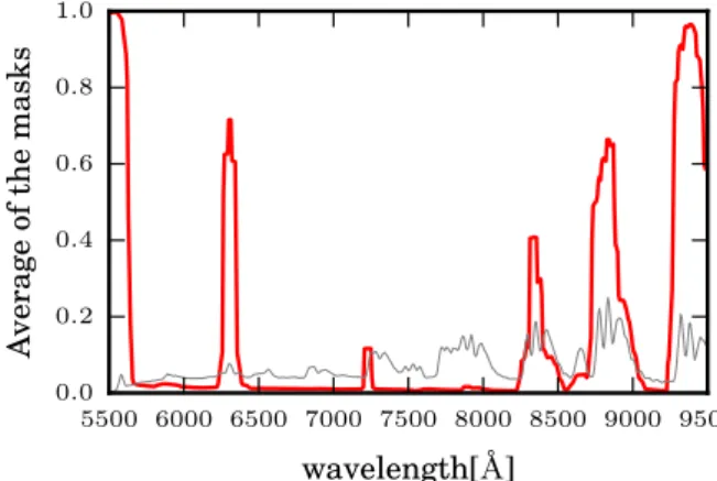
5500 6000 6500 7000 7500 8000 8500 9000 9500 wavelength[ ˚A] 0.0 0.2 0.4 0.6 0.8 1.0 A verage of the masks
Fig. 4. Average of the masks for the VIPERS sample (thick red); a VIPERS sky spectrum is depicted in grey (thin).
1.8σ at wavelengths longer than 7500Å, due to the higher contamination. These thresholds have been chosen empiri-cally: the values were set to select the known sky lines in a subset of representative spectra.
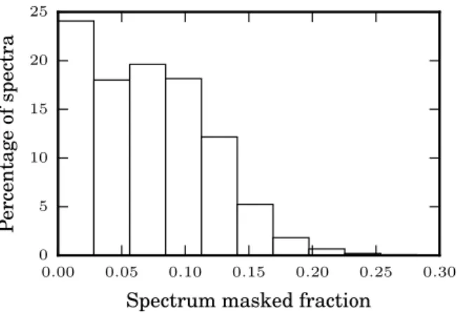
Fig. 4 shows the frequency of masked wavelengths af-ter applying the algorithm to the VIPERS dataset. Around 65% of spectra have been masked in correspondence of the λ=6300Å sky line and of the OH group at ∼ λ=8700Å; about 40% have been masked around λ=8300Å, and only the 10% at ∼ λ=7300Å. Nearly all spectra are masked at the upper and lower wavelength limits of the spectrum, where there is a significant contribution from fringing and calibration issues. In particular, at the lower limit there is the presence of the 5577Å sky line residual combined with the fall-off in the detector sensitivity. The extent of the masking is summarised in Fig. 5. For half of the spectra, the mask covers less than 5% of the wavelength range.
Specifically for the VIPERS spectra, during this phase we also accounted for the extra residuals originating from the subtraction of the zero-order images of bright objects, as shown in the example of Fig. 6. These extra features were identified in the noise spectra delivered by the VIPERS re-duction pipeline through a simple thresholding. Their
po-0.00 0.05 0.10 0.15 0.20 0.25 0.30
Spectrum masked fraction
0 5 10 15 20 25 Percentage of spectra
Fig. 5. Histogram for the distribution of the fraction of masked spectrum after the sky/zero-order residuals masking procedure (the regions at the edges of the spectra have been excluded).
5500 6000 6500 7000 7500 8000 8500 9000 9500 wavelength[ ˚A] 0.0 0.5 1.0 1.5 Flux[erg ·cm − 2s − 1˚ A − 1 ] ×10−17 ID-405051442, z=0.67 Observed spectrum PCA mask Noise spectrum
Fig. 6. Example of zero-order residual in a VIPERS spectrum (top, highlighted by the yellow vertical bar); at the bottom we show the corresponding noise spectrum. The clear excess corre-sponding to the zero-order position is used to supplement the sky residual mask (red line), as to account for this extra contri-bution in the final cleaning and repairing.
sition and size was thus added to the sky residual mask for subsequent treatment.
The process described so far is summarised in the flow chart of Fig. 7.
6. Repairing the spectra
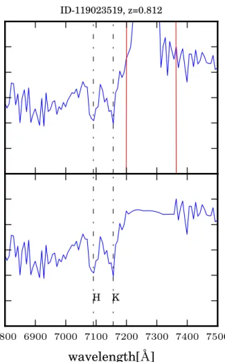
We next compute an estimate for the galaxy continuum in masked regions allowing us to repair the contaminated data. This is helpful not only for visual inspection of the spectra but aids the measurement of spectral features as well. For example, line measurement tools require estimates of the continuum which may be unreliable due to spurious artefacts. Fig. 8(top) shows the D4000 break for a VIPERS spectrum affected by an artefact that prevents the proper measurement of the intensity of the break.
Our approach to reconstruct and repair the spectrum is based on the PCA model in the rest-frame (Marchetti et al. 2013). The shift to rest-frame can only be made if the redshift is known; thus, we apply the procedure only to
A&A proofs: manuscript no. Masking_paper
wavelength[ ˚A]
ID-119023519, z=0.812 6800 6900 7000 7100 7200 7300 7400 7500wavelength[ ˚A]
H KFig. 8. Top panel. Zoom of a VIPERS spectrum with strong residual at the right of D4000Å break. The region of the mask is delimited by the red vertical lines. Bottom panel. The same VIPERS spectrum after repairing the portion affected by the residual.
galaxies with redshift quality flag >= 1. Futhermore, the wavelength range in the rest-frame is limited by the redshift range of the sample. To have sufficient spectra we limit the sample to the redshift range to 0.4 < z < 1.4.
After shifting the spectra to the rest frame, we compute the eigenspectra as described in Marchetti et al. (2013). We use the most significant three eigenvectors to reconstruct the spectra continuum.
The PCA with three components was found to accu-rately reconstruct the continuum of VIPERS spectra in Marchetti et al. (2013). Here we further demonstrate the accuracy of the reconstruction using mock spectra built from linear combinations of Bruzual-Charlot (Bruzual & Charlot 2003) and Kinney-Calzetti (Kinney et al. 1996) templates, also described in Marchetti et al. (2013). The mock spectra were redshifted and degraded with Gaussian noise to mimic the properties of the VIPERS spectra. Us-ing a sample of 20,000 mock spectra we estimated the first three eigenspectra. We then project the mock spectra onto the basis of eigenspectra to compute the reconstruction. We plot an example spectrum in Fig. 9 showing excellent agreement between the model and the reconstruction at all wavelengths. While for the emission lines the discrepancies can be up to ∼25% (Marchetti et al. 2013), the continua
3500 4000 4500 5000 5500 wavelength[ ˚A] −0.005 0.000 0.005 0.010 0.015 0.020 0.025 0.030 0.035 Flux Model Model+noise PCA reconstruction
Fig. 9. Comparison between a model spectrum (orange thick) and the PCA reconstruction of the same spectrum (thin green) after degrading it with noise (in soft grey the degraded spec-trum). ID-116117443, z=1.03 Observed spectrum 5500 6000 6500 7000 7500 8000 8500 9000 9500 wavelength [ ˚A] Repaired spectrum
Fig. 10. Example of a VIPERS spectrum (blue) and the cor-responding mask (red straight lines) (top panel) and its PCA repairing in the masked portions (bottom).
are always well reproduced; in particular from the test spec-tra, we found that the discrepancies between reconstructed and model continua are on average lower than ∼1.6%, and are never worse than ∼5%, where such a discrepancy is ob-tained in rare cases (< 0.1%).
Since the intensity of line features cannot be reproduced precisely we introduce a “line safeguard” and do not use the reconstruction at the locations of known features. For VIPERS we ensure that the reconstruction does not sub-stitute the most prominent emission lines (e.g. [OII], Hβ, [OIIIa], [OIIIb], Hα for galaxies), and the D4000 break. The safeguard was necessary for 30% of VIPERS spectra for which a mask fell on a known feature.
An example of rest-frame repairing within the mask re-gions is shown in Fig. 10. After the repairing, the deter-mination of the intensity of the galaxy spectral features is easier and more reliable, as shown in Fig. 8 bottom.
Not all spectra may be repaired using this procedure; sources outside the redshift range 0.4 < z < 1.2 or sources without a measured redshift cannot be modeled using the PCA. For these sources we use a constant interpolation
Fig. 11. A VIPERS stellar spectrum repaired with points at constant value at the level of the continuum, computed near the regions of the mask (red).
to repair the masked regions, see Fig. 11. Additionally, for active galaxies (AGN), the PCA reconstruction based upon galaxy eigenspectra is not applicable. Marchetti et al. (2013) found that the eigenspectra computed from the full survey could not represent rare AGN spectra well. Thus, for VIPERS spectra identified as AGN we have used con-stant interpolation to repair the masked regions. The steps followed to create the automatic repairing described here are schematically listed in the flow chart of Fig. 12.
7. Comparison and combination of automatic and
manual cleaning for the VIPERS data
For VIPERS spectra, a significant amount of time has been spent by the VIPERS team to manually clean the spec-tra from sky residuals or other artifacts, producing many careful manual edits. To check the reliability and efficiency of the automatic procedure, we compared ∼ 500 automati-cally masked and repaired spectra with their corresponding manually edited spectra.
Fig. 13 shows this comparison for two spectra of dif-ferent quality. The black spectrum in the upper plot of Fig. 13-top is a high signal-to-noise sky subtracted trum; the corresponding statistical PCA sky residuals spec-trum is overplotted in cyan; the red line shows the mask as computed by the cleaning procedure. The resulting auto-matically masked and PCA repaired spectrum is shown in the middle plot of Fig. 13-top (blue): within the regions of the mask, the observed spectrum has been replaced by the corresponding portion of the rest-frame PCA cleaned spectrum. The black dotted-dashed vertical lines highlight the wavelengths where some important emission lines are expected given the redshift. In these regions the repairing (if any) is not applied. The lower plot of Fig. 13-top shows the manually edited spectrum. Overall, the automatically cleaned and repaired spectrum is very similar to the manu-ally edited one. In the region of strong OH lines, the PCA cleaning looks more aggressive because the reconstructed portion of the spectrum is noise free while the human se-lectively edited the spurious features.
The bottom group of panels of Fig. 13 is like the pre-vious, but shows a spectrum with lower signal to noise. In this case, the automatic cleaning is more precise with
re-Fig. 12. Scheme of the automatic repairing procedure
spect to the manual cleaning, especially around the 6300Å sky line and the zero order spectrum at 8700Å.
8. Conclusions
We have presented a novel algorithm based upon princi-pal component analysis to identify and repair spectral de-fects (such as those deriving from a non-perfect sky subtrac-tion) in large sets of galaxy spectra. We have implemented the procedure for the VIPERS dataset and tested its per-formance extensively against conventional manual spectral masking. The data products produced by this work are part
A&A proofs: manuscript no. Masking_paper
Fig. 13. Cleaning of a Flag 4 (top) and a Flag2 (bottom) VIPERS spectrum: for each panel, the upper plot is the observed (sky subtracted) spectrum (thick black), superposed to the mask (red straight lines) and the rescaled sky residuals spectrum (thin cyan); the middle plot shows the automatic cleaning, with the expected position of the [OII], Hβ and [OIII] lines marked in black by the dash-dotted lines; the bottom plot is the manually edited spectrum.
of the VIPERS second data release (PDR-2) (Scodeggio et al. 2016).
The PCA algorithm characterizes a dataset with a com-pact set of components without specification of a model. These components can represent the signal of interest but may also describe unwanted systematic effects as we ex-plored in this work. With the advent of spectroscopic sur-veys collecting millions of spectra, the use of automated procedures is becoming unavoidable to guarantee the effi-cient and accurate treatment of the data.
References
Bruzual, G. & Charlot, S. 2003, MNRAS, 344, 1000
Colless, M., Dalton, G., Maddox, S., et al. 2001, MNRAS, 328, 1039 Connolly, A. J., Szalay, A. S., Bershady, M. A., Kinney, A. L., &
Calzetti, D. 1995, AJ, 110, 1071
Cucciati, O., Davidzon, I., Bolzonella, M., et al. 2016, ArXiv e-print 1611.07049
de la Torre, S. et al. 2016, A&A submitted, ArXiv e-print XXXX.YYYY
Garilli, B., Fumana, M., Franzetti, P., et al. 2010, PASP, 122, 827 Garilli, B., Guzzo, L., Scodeggio, M., et al. 2014, A&A, 562, A23 Garilli, B., Le Fèvre, O., Guzzo, L., et al. 2008, A&A, 486, 683 Guzzo, L., Scodeggio, M., Garilli, B., et al. 2014, A&A, 566, A108 Hawken, A. J., Granett, B. R., Iovino, A., et al. 2016, ArXiv e-print
1611.07046
Karhunen, H. 1947, Ann. Acad. Science Fenn, A.I, 37
Kinney, A. L., Calzetti, D., Bohlin, R. C., et al. 1996, ApJ, 467, 38 Le Fèvre, O., Saisse, M., Mancini, D., et al. 2003, in Proc. SPIE, ed.
M. Iye & A. F. M. Moorwood, Vol. 4841, 1670–1681
Le Fèvre, O., Vettolani, G., Garilli, B., et al. 2005, A&A, 439, 845 Lilly, S. J., Le Brun, V., Maier, C., et al. 2009, ApJS, 184, 218 Marchetti, A., Granett, B. R., Guzzo, L., et al. 2013, MNRAS, 428,
1424
Newman, J. A., Cooper, M. C., Davis, M., et al. 2013, ApJS, 208, 5 Pezzotta, A. et al. 2016, A&A submitted, ArXiv e-print XXXX.YYYY Scodeggio, M., Franzetti, P., Garilli, B., Le Fèvre, O., & Guzzo, L.
2009, The Messenger, 135, 13
Scodeggio, M., Franzetti, P., Garilli, B., et al. 2005, PASP, 117, 1284 Scodeggio, M., Guzzo, L., Garilli, B., et al. 2016, ArXiv e-print
1611.07048
Stoughton, C., Lupton, R. H., Bernardi, M., et al. 2002, AJ, 123, 485 Wild, V. & Hewett, P. C. 2005, MNRAS, 358, 1083
Wilson, M. et al. 2016, A&A submitted, arXiv:XXXX.YYYY Yip, C. W., Connolly, A. J., Szalay, A. S., et al. 2004, AJ, 128, 585 York, D. G., Adelman, J., Anderson, J. J. E., et al. 2000, AJ, 120,
1579
1 2
INAF - Istituto di Astrofisica Spaziale e Fisica Cosmica Mi-lano, via Bassini 15, 20133 MiMi-lano, Italy INAF - Osservatorio
Astronomico di Brera, Via Brera 28, 20122 Milano – via E. Bianchi 46, 23807 Merate, Italy
3 Università degli Studi di Milano, via G. Celoria 16, 20133
Milano, Italy
4
INAF - Osservatorio Astronomico di Bologna, via Ranzani 1, I-40127, Bologna, Italy
5
Aix Marseille Univ, CNRS, LAM, Laboratoire
d’Astrophysique de Marseille, Marseille, France
6
INAF - Osservatorio Astrofisico di Torino, 10025 Pino Tori-nese, Italy
7
Laboratoire Lagrange, UMR7293, Université de Nice Sophia Antipolis, CNRS, Observatoire de la Côte d’Azur, 06300 Nice, France
8
Institute of Physics, Jan Kochanowski University, ul. Swi-etokrzyska 15, 25-406 Kielce, Poland
9
National Centre for Nuclear Research, ul. Hoza 69, 00-681 Warszawa, Poland
10 Dipartimento di Fisica e Astronomia - Alma Mater
Studio-rum Università di Bologna, viale Berti Pichat 6/2, I-40127 Bologna, Italy
11 INFN, Sezione di Bologna, viale Berti Pichat 6/2, I-40127
Bologna, Italy
12
Aix-Marseille Université, Jardin du Pharo, 58 bd Charles Livon, F-13284 Marseille cedex 7, France
13
IRAP, 9 av. du colonel Roche, BP 44346, F-31028 Toulouse cedex 4, France
14
Astronomical Observatory of the Jagiellonian University, Orla 171, 30-001 Cracow, Poland
15
School of Physics and Astronomy, University of St Andrews, St Andrews KY16 9SS, UK
16
INAF - Istituto di Astrofisica Spaziale e Fisica Cosmica Bologna, via Gobetti 101, I-40129 Bologna, Italy
17
INAF - Istituto di Radioastronomia, via Gobetti 101, I-40129, Bologna, Italy
18 Canada-France-Hawaii Telescope, 65–1238 Mamalahoa
High-way, Kamuela, HI 96743, USA
19 Aix Marseille Univ, Univ Toulon, CNRS, CPT, Marseille,
France
20 Dipartimento di Matematica e Fisica, Università degli Studi
Roma Tre, via della Vasca Navale 84, 00146 Roma, Italy
21
INFN, Sezione di Roma Tre, via della Vasca Navale 84, I-00146 Roma, Italy
22
INAF - Osservatorio Astronomico di Roma, via Frascati 33, I-00040 Monte Porzio Catone (RM), Italy
23
Department of Astronomy, University of Geneva, ch.
d’Ecogia 16, 1290 Versoix, Switzerland
24
INAF - Osservatorio Astronomico di Trieste, via G. B. Tiepolo 11, 34143 Trieste, Italy
25
Department of Astronomy & Physics, Saint Mary’s Uni-versity, 923 Robie Street, Halifax, Nova Scotia, B3H 3C3, Canada
26
Institute of Cosmology and Gravitation, Dennis Sciama
Building, University of Portsmouth, Burnaby Road,
Portsmouth, PO13FX
27 Institut Universitaire de France
28 Institute d’Astrophysique de Paris, UMR7095 CNRS,
Uni-versité Pierre et Marie Curie, 98 bis Boulevard Arago, 75014 Paris, France
29
Institute for Astronomy, University of Edinburgh, Royal Ob-servatory, Blackford Hill, Edinburgh EH9 3HJ, UK