Passive and Active Coupling Comparison of Fuel Cell and
Supercapacitor for a Three-Wheel Electric Vehicle
A. Macias1*, M. Kandidayeni1, L. Boulon1,2, J. Trovão3,4
1 Université du Québec à Trois-Rivières, Hydrogen Research Institute, Trois-Rivières, QC,
Canada
2 Canada Research Chair in Energy Sources for the Vehicles of the Future
3 e-TESC Laboratory, Dept. Electrical & Computer Engineering, University of Sherbrooke,
Sherbrooke, QC, J1K 2R1, Canada
4 Canada Research Chair in Efficient Electric Vehicles with Hybridized Energy Storage
Systems
[*]Corresponding author: alvaro.omar.macias.fernandez@uqtr.ca
This is the peer reviewed version of the following article: Macías, A., Kandidayeni, M., Boulon, L., & Trovão, J. (2020). Passive and Active Coupling Comparison of Fuel Cell and Supercapacitor for a Three-Wheel Electric Vehicle. Fuel Cells, 20(3), 351-361, which has been published in final form at http://dx.doi.org/10.1002/fuce.201900089. This article may be used for non-commercial purposes in accordance with Wiley Terms and Conditions for Use of Self-Archived Versions.
Abstract
The desire to reduce the power electronics related issues has turned the attentions to passive coupling of powertrain components in fuel cell hybrid electric vehicles (FCHEVs). In the passive coupling, the fuel cell (FC) stack is directly connected to an energy storage system on the DC bus as opposed to the active configuration where a DC-DC converter couples the FC stack to the DC bus. This paper compares the use of passive and active couplings in a three-wheel FCHEV to reveal their strengths and weaknesses. In this respect, a passive
configuration, using a FC stack and a supercapacitor, is suggested first through formulating a sizing problem. Subsequently, the components are connected in an active configuration where an optimized fuzzy energy management strategy is used to split the power between the
components. The performance of the vehicle is compared at each case in terms of capital cost and trip cost, which is composed of FC degradation and hydrogen consumption, and total cost of the system per hour. The obtained results show the superior performance of the passive configuration by 17% in terms of total hourly cost, while the active one only results in less degradation rate in the FC system.
Keywords: Active Configuration, Electric Vehicles, Fuel Cell, Hybridization, Hydrogen Car,
1 Introduction
Conventional vehicles powered by fossil fuels are considered as major contributors to air pollution and have made transportation one of the main responsible sectors for CO2 emissions
[1]. While the air pollution poses considerable risks for human health and environment, its harmful effects can be mitigated through electrification of transport systems [2]. Among the existing technologies, such as electric vehicles, hybrid electric vehicles etc., FC vehicle is one of the most auspicious due to zero-local emissions, high level of driving autonomy, and fast refueling time [3]. However, FC systems cannot tolerate sudden and significant fluctuations in the load which are normal in vehicular applications [4]. The load peaks can cause air/fuel starvation in the FC system resulting in serious power drop [5, 6]. Furthermore, abrupt
changes in the load have detrimental effects on the lifetime of the FC stack since it accelerates the degradation rate of the system [7, 8]. Hybridization of a FC system with other sources, such as batteries and supercapacitors (SCs), has been widely used in the literature to alleviate the problems regarding the slow dynamic essence of a FC system [9]. The main goal of this hybridization is to supply the power peaks with an energy storage device and benefit from the regenerative braking mechanism. Different hybridization configurations can be found in the literature [10-13]. In [12], a review of six topologies, which can be mainly fallen into two categories of active and passive, for a FCHEV is presented. Active configuration refers to the connection of the power source to the DC bus via a converter. In active configurations, normally, an energy management strategy (EMS) is required to perform the power split among the components while satisfying the requested power. Several EMSs from rule based and optimization based to intelligent based strategies have been proposed for such
configuration [14]. Among them, fuzzy logic control (FLC) is one of the most commonly used due to the flexibility, robustness, and convenient implementation [15]. FLCs provide strategic rules by using linguistic labels. Several grounds, such as inaccurate model of a vehicle’s components, nonlinearity, and unknown aspects, like traffic, weather, etc., can be
mentioned for appropriateness of employing a FLC in FCHEV application. Contrary to the active configuration, passive coupling refers to the connection of the component directly to the DC bus. This kind of architecture is independent of an EMS and has self-management due to the characteristics (different impedance) of the components. The passive configuration provides similar benefits as the active architecture while it does not require any DC-DC converter saving of weight, cost, and energy losses linked with an extra level of power conversion. However, the drawback of the passive hybrid system is that the FC stack is the main responsible for supplying the requested traction power as there is no controlled power regulation among the power sources. The power split between the FC system and the SCs depends on the natural behavior of each source (internal resistor and open circuit voltage for instance). Therefore, several authors refer to it as “natural energy management” [16, 17]. This can lead to the presence of higher power ripples at the FC side and consequently increase the degradation rate of the stack. In [10], the comparison of active and passive hybrid
configurations of FC and battery, as an auxiliary power unit of trucks, reveals that the direct coupling of FC and battery has a better performance as long as the demanded power does not have substantial variations. However, marked fluctuations of the demanded power can make the FC operate in low-efficiency regions. The selection of active and passive configurations has been considered in a FCHEV, using a SC bank and a battery pack as the secondary power source units [11]. This study demonstrates that the active coupling of the battery with the FC stack leads to high power variations in the stack while the passive connection of FC-SC makes the requested power from the FC smoother and has a higher energetic efficiency. Although active configuration provides a better management of the components, several researchers have opted to use passive connections to reduce the complexity, cost, and weight of the system [18]. In this among, the direct connection of FC with SC, as an energy storage system, is more prevalent, compared to the battery, due to the capability of a SC in coping with intermittency of behavior in FCHEV applications. In [19-21], the main focus is on the
direct hybridization of SC to a single FC. The obtained experimental results indicate that the passive connection avoids negative voltage, provides self-protection against sudden power changes, increases the dynamic of the system, and enhances the electrical performance as patented by NISSAN company [22]. In [23], the performed study takes the arrangement of SCs into consideration in the passive configuration and concludes that increasing the number of SCs reduces the power supplied by the FC as well as the hydrogen consumption, while escalating the capital cos of the system. In [24, 25], the FC-SC passive coupling is specifically used for the vehicular application. In [26], the simulation results show that the direct
hybridization of FC-SC benefits from high fuel economy and recovers more regenerative energy than battery due to its low internal resistance. In [27], the experimental results of a 9.5-kW proton exchange membrane FC (PEMFC) passively coupled with a SC array illustrate a reduction in dynamic load, idling time, and rapid load changes in the FC without using a DC/DC converter.
In the light of the discussed manuscripts, it is obvious that some attempts have been already done regarding the direct coupling of FC and SC in vehicular applications. However, such a coupling has never been used for a recreational three-wheel electric vehicle so far. These types of vehicles are normally exposed to high dynamics and need to be light and compact. The thing that makes the choice of passive couplings interesting here is that these
configurations provide low mass and compactness through the elimination of power electronics. Moreover, SC, which is a prevalent component in this kind of configuration, is highly capable of dealing with high dynamics. In this regard, a comparative analysis of FC-SC passive and active configurations for a three-wheel vehicle, which has more power demand variation than conventional vehicles, is put forward in this manuscript. To do so, firstly, the minimum required size of the main components is determined in order to meet the requested power since this type of vehicle is expected to have low mass and volume.
selected components in both of passive and active configurations. Passive configuration benefits from self-management and does not require the design of an EMS. However, in the active configuration, the power split is performed by using an optimized fuzzy strategy. As opposed to other similar works which only use the hydrogen consumption as a means of comparison, a detailed performance index based on capital cost and trip cost of the system is defined in this work. Moreover, a real driving cycle from the three-wheel electric vehicle is utilized to carry out the simulation.
The remainder of this paper is organized as follows. The vehicle modeling with passive and active configurations is described in Section 2. The designed EMS for the active configuration is presented in Section 3. The obtained results of the comparative analysis are discussed in Section 4. Finally, the conclusion is given in Section 5.
2 Modeling
2.1 Components sizing
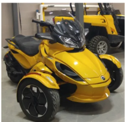
The studied vehicle in this paper (e-TESC-3W platform shown in Figure 1) is a three-wheel electric vehicle used essentially for leisure purposes. This prototype is currently used as a test bench at e-TESC laboratory of University of Sherbrooke [28]. The e-TESC-3W platform has a 28-kW (96 V) permanent magnet synchronous motor (PMSM) directly connected to the rear wheel. The main specifications of this vehicle are listed in Table 1 and explained thoroughly in [28]. This vehicle can reach a maximum speed of 120 km h-1.
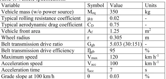
Table 1: Vehicle specifications
Variable Symbol Value Units
Vehicle mass (w/o power source) Meq 350 kg
Typical rolling resistance coefficient µfr 0.02 -
Typical aerodynamic drag coefficient CD 0.75 -
Vehicle front area Af 1.25 m2
Wheel radius r 0.305 m
Belt transmission drive ratio Ggb 5.033 (30:151) -
Belt transmission drive efficiency Ƞgb 95 %
Maximum speed Vmax 120 km h-1
Acceleration speed Vacc 100 km h-1
Acceleration time tacc 7 s
Grade slope at 100 km/h θ 0.03 %
Originally, e-TESC-3W platform has been a pure battery electric vehicle (BEV). In [29], a coupling of battery, as the main power source, and the SC, as the energy storage system, is proposed for this vehicle where battery supplies the average power while the SC is held responsible for the high dynamic phase. The authors in [29] indicate that their proposed hybrid configuration can enhance the lifetime of the e-TESC 3W platform powertrain components compared to the pure BEV. The principal objective of the current manuscript is to provide a comparison of passive and active FC-SC powertrain configurations for the e-TESC 3W platform. To do so, initially, performing a component sizing to figure out the rated power of the FC and SC in relation to the requirements of the vehicle is necessary. Leisure activity vehicles are typically characterized as being light and compact, but with a high acceleration and speed capabilities. In this regard, the sizing problem should ascertain the minimum required component dimensions to satisfy the requested power for all the constraints specified in Table 2 [30].
Table 2: FC stack and SC characteristics
Component Parameter Variable Value Units
FC
No. cells Ncell 135 Cells
Max power PFC,max 27.3 kW
Max current iFC,max 300 A
OCV voltage VFC,OCV 130.2 V
Max temperature TFC,max 70 °C
Thermal capacity MCfc 140 kJ K-1
Stack mass FCmass 19.5 kg
Current slew rate FCSR 20 As-1
SC
No. SC in series SCserie 50
SC mass SCmass 510 gr
Equivalent series resistance (ESR) SCESR 0.29 mΩ
Capacitance SCc 3000 F
Rated voltage SCv,rated 2.7 V
Max current SCMax,i 1900 A
Cut-off frequency SCcut-off 26 mHz
Based on the specifications, the FC needs to be sized in a way to supply the maximum power for a long distance, continuous, and high-speed driving. Otherwise the SC will get discharged quickly [31]. The FC supplies the base power (Pe) in the maximum speed condition premised
on the hybrid vehicle traction force resistance (Fenv) as:
Pe = Fenv VEV/(1000ƞt ƞem) (1)
Fenv = Froll + Fgrade + Fair (2)
Froll = Meq g µfr cos(θ) (3)
Fair = 0.5ρa Af Cd VEV2 (4)
Fgrade = Meq g sin(θ) (6)
where Froll is the rolling resistance force, Fgrade is the grade related force, Fair is the resistance
force against the air, Meq is the mass of the vehicle, g is gravity, µfr is the rolling resistance
coefficient, ρa is the air density, Cd is the aerodynamic drag coefficient, Af is the frontal area,
VEV is the vehicle speed, θ is the road grade, ƞt is the transmission efficiency, and ƞem is the
motor average efficiency [32]. Solving Eq. (1) leads to the value of 26.5 kW for Pe under
maximum speed condition (120 km h-1) on a flat road. This value defines the size of the FC
for steady conditions. Moreover, the maximum electric power for the vehicle acceleration from 0 to 120 km h-1 in 7 seconds comes to 88 kW on a flat road, obtained by:
Ptot = (Froll + Fgrade + Fair + Facc) VEV /(1000 ƞt ƞem) (7)
Facc = Meq δ d VEV /dt (8)
where Facc is the accelerating force, and δ is the mass factor related to the rotational inertia. δ
is assumed to be 1.035 for a one-speed gear-box [33].
With respect to the calculated Ptot, the minimum SC size should be 60.7 kW while the selected
FC size is 27.3 kW (FCvelocity-9SSL) from Ballard [34, 35]. The utilized SC in this work is K2 Series from Maxwell Technologies [24]. The characteristics of the selected components are listed in Table 2.
It is worth reminding that due to the direct connection of the SC bank and FC stack in passive configuration, the SC nominal voltage needs to be higher than the open circuit voltage of the FC. In this respect, the studied system requires 50 SCs connected in series. Regarding the active configuration, a 30-kW DC/DC converter (non-isolated) with a mass around 11 kg is used [36].
The tank size selection is done by assuming a similar autonomy as the pure electric e-TESC 3W platform, which is around 150 km for a full charge. Taking into account this autonomy and the performance of the FC system in the lowest efficient zone, which is at the maximum speed of 120 km h-1, the required hydrogen would be 1.77 kg. Based on the targets
of light-duty fuel cell vehicles of DOE, the system volumetric capacity of the tank in 2020 should be 0.040 kg H2 L-1 [37]. Therefore, the weight of the high-pressure tank in this
manuscript comes to 32.2 kg.
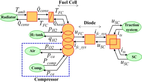
2.2 Energetic Macroscopic Representation
In this manuscript, energetic macroscopic representation (EMR), which is a graphical method to organize the model of complex multiphysics systems, is used to model the e-TESC 3W platform in both active and passive configurations [38, 39]. The traction system of
e-TESC 3W platform vehicle is shown in Figure 2. Passive and active energy source
subsystems (ESSs) are presented in Figure 3 and Figure 4 respectively. According to Figure 2, the hybrid vehicle velocity can be derived from the traction force and traction force resistance as [28]: Meq dVEV/dt = Ftr – Fenv (9) Ftr = (Ggb/r) Tem ƞgbζ (10) Ωm = (Ggb/r) VEV (11) ζ = 1, for Tem ≥ 0 (12) ζ = -1, for Tem < 0 (13) Tem = Tem_r (14)
where Ftr is the traction force, Ggb is the gearbox transmission ratio, r is the wheel radius, Tem is the electric machine torque, ƞgb is theGearbox transmission efficiency,Ωm is the rotor rotation speed, andTem_r is a reference torque to control the electric machine. The requested current of the vehicle from the electric motor side (its) is then formulated as: its = (Tem Ωm ƞmβ)/USC (15)
where USC is the SC voltage. In the passive configuration, as it can be seen in Figure 3, there is no DC-DC converter and a diode is used in series with the PEMFC stack to prevent the reversed current. The equivalent resistor of the diode (rD) along with the voltage difference of the FC (Ufc) and SC (USC) determine the current of the FC system (iFC-sys). iFC-sys = (Ufc -USC)/rD (16)
its = iFC-sys + iSC (17)
where iSC is the current of the SC. On the other hand, in the active configuration, as shown in
Figure 4, the current goes through a converter as [36]:
iFC-sys Vfc = idc/dc USC ƞdc/dc (18)
its = idc/dc + iSC (19)
Figure 2: Traction system of the e-TESC 3W platform vehicle
Figure 4: The utilized active ESS of e-TESC 3W platform vehicle
where idc/dc is the converter current and ƞdc/dc is the converter efficiency.
The PEMFC voltage (Ufc) is calculated by using the semi-empirical model suggested in [40].
Ufc = Ncell × (ENernst + Uact + Uohmic + Ucon) (20)
ENernst = 1.229 – 0.85×10⁻³ (Tfc – 298.15) + 4.3085 × 10⁻⁵ Tfc[ln(pH2) + 0.5ln(pO2)] (21)
Uact = ϒ1 + ϒ2 Tfc + ϒ3 Tfc ln(CO2) + ϒ4 Tfc ln(iFC) (22)
CO2 = pO2/5.08×106 e-(498/Tfc) (23)
Uohmic = - iFC Rinternal = - iFC (ξ1 + ξ2 Tfc + ξ3 iFC) (24)
Ucon = α iFCGln(1 – β iFC) (25)
where ENernst is the reversible voltage, Uact is the activation loss, Uohmic is the ohmic loss,Ucon
is the concentration loss, Tfc is the stack temperature, pH2 is the hydrogen partial pressure, pO2
is the oxygen partial pressure, ϒn (n = 1 … 4) is the empirical coefficients, CO2 is the oxygen
concentration, ifc is the the FC operating current, Rinternal is the internal resistor defined by the
diffusion mechanism (0.3≤ α ≤1.8), G is a dimensionless number related to the water flooding phenomena (1≤ G ≤4), and β is the inverse of the limiting current.
The thermal behavior of the stack is modeled by using the energy conservation law. The energy balance for describing the temperature dynamic of the PEMFC can be given by [41]:
Qheat=Nfc ifc(1.254 – Ufc) (26)
Hfc=(Nfc/36)(2700kt1 + kt2) (27)
Qconv=Hfc(Tfc – Tamb) (28)
dTfc/dt = (Qheat – Qconv)/MCfc (29)
where Qheat is the generated heat in the FC, Nfc is the number of cells, Hfc is the heat transfer coefficient, kt1 and kt2 are the coefficiencts obtained experimentally in [41], Tamb is the ambient temperature, Tfc is the stack temperature, Qconv is the convection heat transfer, and MCfc is the thermal capacity of the FC. The current of the PEMFC system (iFC-sys) is obtained by considering the losses from the balance of plant as [41, 42]: iFC-sys = (Pfc – Pcomp – Pfan)/Ufc (30)
Pcomp = ƞcomp-1 Wair cp Tamb ((pca/pamb)^((γ-1)/γ)-1) (31)
Pfc = Ufc ifc (32) Wair = λ WO2/χO2 (33) WO2 = MO2 Nfc ifc/2F (34) pO2 = 0.21pca (35) pH2 = 0.99pan (36) pca = a1 + a2ifc + a3ifc2+ a3ifc3 (37) pan = pca + 20000 (38)
where Pcomp is the consumed power by the compressor, pca is the pressure in the cathode, Pfan is
the consumed power by the FC fan (200 W), ƞcomp is considered as the average compressor
efficiency (0.70) [43], Wair is the rate of used air, cp is the air specific heat capacity (1005 JK -1), p
amb is the ambient pressure, γ is the ratio of specific heats of air (1.4), λ is the oxygen
excess ratio which is two, WO2 is the oxygen consumption rate, χO2 is the oxygen mass
fraction (0.233), MO2 is oxygen molar mass, F is the Faraday constant, pan is the pressure in
the anode, and ai(i=1…3) is the experimentally obtained coefficient.
The hydrogen flow (qH2) is calculated based on an experimental formula as [34]:
qH2 = 0.00696ifc Nfc (39)
Based on the mentioned models, the efficiency of the FC system is calculated considering the power losses of the auxiliaries:
Ƞsys = (Pfc – Pcomp – Pfan)/(qH2 HHV) (40)
where the generated hydrogen power is the product of hydrogen flow and the high heating value of hydrogen (HHV=286 kJ mol-1). In the active coupling, the converter efficiency is
multiplied by the FC system efficiency to know the efficiency in the DC bus. Finally, the SC is modeled based on the equivalent circuit proposed in [44].
USC=rSC iSC + (1/CSC) ∫ iscdt (41)
2.3 Degradation
One of the most significant factors while using a FC system as the main power source of a vehicle is durability consideration. This is mainly due to the fact that FC is really damage prone although it is one of the costly components of the powertrain. In automotive
applications, the end of life (EOL) of a FC stack is defined when a 10% voltage loss is reached [45]. For this reason, it is vital to include the degradation of the FC stack in the analysis of the system performance. According to [25, 46, 47], the causes of FC degradation fit into five cases of load changing, startup and shutdown, low power load (idle condition), high power load, and natural decay. An empirical model for determining the voltage degradation of the FC stack can be formulated as [46]:
∆𝐹𝐶deg = ∆𝐹𝐶𝑛at +∆𝐹𝐶𝑎𝑑𝑑 (42)
where ∆𝐹𝐶deg denotes the degradation of the FC in percentage, ∆𝐹𝐶𝑛at is the natural decay rate
related to the expected lifetime of the FC in normal operation conditions, and ∆𝐹𝐶𝑎𝑑𝑑 is the
degradations rooted from unfavourable operations.
The influence of each factor on the degradation of the FC can be defined as:
∆𝐹𝐶𝑑𝑒𝑔 = 𝑘1 𝑡1 + 𝑘2 𝑛1 + 𝑘3 𝑡2 + 𝑘4 t3 + βnat 𝑡𝐹𝐶_𝑂𝑁 (43)
where t1 is the idle time, n1 is the number of start-stops, t2 is the duration of heavy loading,
and t3 is the time in high power condition. The idle condition is described as the output power
which is less than 5% of maximum power (PLow), the heavy loading is an absolute variation
more than 10% of maximum power per second, and high power is delimited as higher than 90% of maximum power (PHigh). Based on the 2020 FC lifetime target of DOE (5000 hours),
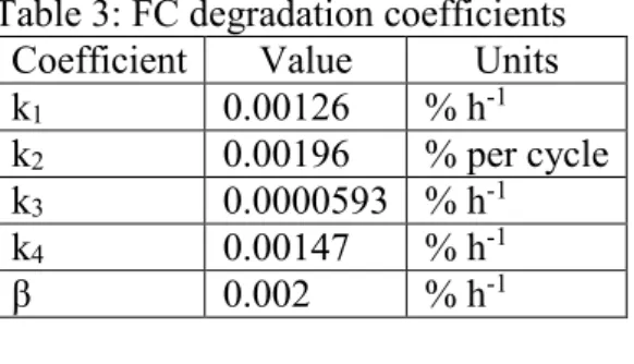
the natural decay rate βnat is set to reach a voltage loss of 10% in 5000 hours [48]. Table 3
In addition to the FC stack, a calendar degradation model has been considered for the SC based on the datasheet of the manufacturer. According to this datasheet, the expected lifetime of this device is 10 years. Moreover, the EOL of the SOC is defined as an increment of 100% in SCESR and a decrement of 20% in SCC [24].
Table 3: FC degradation coefficients
Coefficient Value Units
k1 0.00126 % h-1
k2 0.00196 % per cycle
k3 0.0000593 % h-1
k4 0.00147 % h-1
β 0.002 % h-1
3 Energy management strategy for active coupling
As explained earlier, the main purpose of this work is to compare the use of FC-SC passive and active couplings for the e-TESC 3W platform vehicle. Passive configuration does not need an EMS as the operating current harmonics are chiefly provided by the component with the lowest impedance, SC herein, in such configuration. However, to bring into attention the strengths of the utilized passive architecture, its performance is compared with an active configuration where the same selected FC stack is connected to the DC bus through a DC-DC converter and the SC is directly connected to the bus. Such active configuration needs an EMS to split the power between the FC and SC. In this respect, a FLC based EMS is designed and optimized by genetic algorithm (GA) for the purpose of this paper. FLC uses some if-then rules to integrate the knowledge of an expert into the design procedure and does not require a precise model of the system. Since the comparative analysis of this work is mainly based on a specific real deriving cycle, the parameters of the FLC has been adjusted by GA to improve its performance as much as possible for this known driving cycle.
The designed FLC for the purpose of power splitting in the active powertrain of this work has two inputs, requested power and SC voltage, and one output, which is the required power from the FC. The input and output membership functions (MFs) of the FLC as well as the
fuzzy reasoning rules are tuned by GA. Since the optimization of FLC is a common approach in the literature [49, 50], its explanation has been considered unnecessary in this manuscript. The proposed cost function for optimizing the performance of the FLC is as follows.
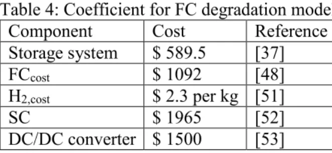
CTrip = FCcost ΔFC + H2,cost Hcons (44)
where FCcost is the cost of the FC, specified in Table 4, ΔFC is the degradation percentage of
the FC, obtained by Eq. (43), H2,cost is the cost per kilogram of hydrogen, and Hcons is the
hydrogen consumed during the trip. Table 4 shows the cost breakdown of the complete power source system.
Table 4: Coefficient for FC degradation model
Component Cost Reference
Storage system $ 589.5 [37]
FCcost $ 1092 [48]
H2,cost $ 2.3 per kg [51]
SC $ 1965 [52]
DC/DC converter $ 1500 [53]
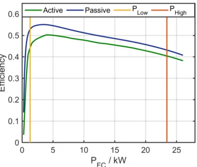
Figure 5 shows the comparison of the FC system efficiency between active and passive configurations. According to this figure, the overall efficiency of the passive system is higher than the active system due to the exclusion of the power electronic related losses. Figure 5 also delimits the low power (PLow) zone, which is 5% of the maximum power, and high power
(PHigh) zone, which is 90% of the maximum power. For both cases of passive and active
Figure 5: FC system efficiency comparison of active and passive couplings
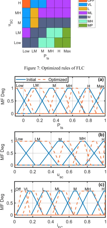
The optimization process has been carried out for a real driving cycle recorded from e-TESC 3W platform shown in Figure 6. The optimized reasoning rules of the FLC are
presented in Figure 7. From this figure, it is clear that the optimized EMS avoids unnecessary on-off cycles. Indeed, it keeps the FC stack in a very low (VL) power mode when the
requested power is low, and the voltage of the SC is high. Moreover, the FC stack tries to maintain the SC voltage in high levels in order to embrace any sudden peaks of power.
Figure 8 shows the initial and optimized MFs of the two inputs and one output. Regarding the MFs of the first input (Pts) and the output (IFC), it can be seen that they have almost formed an
equal distribution over the universe of discourse. On the contrary, in the second input (USC),
the low level covers up to 40% of the range of value. This range implies that the optimization algorithm has opted to keep the SC within a high level of energy to deal with the high
dynamics behavior of the profile. In order to clarify the obtained shape in the MFs of the optimized fuzzy, it should be reminded that a trapezoidal MF can be defined as Trapezoidal (x; a, b, c, d, while a < b < c < d):
0 x < a (45)
m1 = x-a/b-a a≤ x ≤ b (46)
1 b≤ x ≤c (47)
m2 = d-x/d-c c≤ x ≤d (48)
0 d ≤x (49)
where x represents real value (Crisp Value) within the universe of discourse while a, b, c, d represent a x-coordinates of the four heads of the trapezoidal. During the optimization process of this work, the two constructing slopes of each trapezoidal MF (m1 and m2) has been forced
to reach the same value.
Figure 7: Optimized rules of FLC
Figure 8: Optimized FLC MFs, a) requested power (input 1), b) voltage of SC (input 2), and c) required current from the FC (output)
4 Results and discussion
The achieved results of the carried out comparative study is presented in this section. Primarily, the results related to the split and distribution of the power among the power sources are investigated. Secondly, the cost of FC degradation and hydrogen consumption are compared for each of the configurations. Finally, other aspects, such as the trip cost, total cost of the system, and hourly system cost, are compared for each case study.
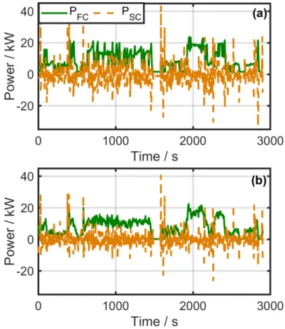
Figure 9 shows the power split between the FC stack and SC bank in each configuration. Comparison of the active and passive configurations shows that in the active coupling, the SC operates in a wider range which leads to the high efficiency performance of the FC stack. Regarding the passive coupling, it is clear that the extracted power from the FC stack follows a smoother path since the SC bank functions as a low-pass filter in such configurations. It is worth mentioning that both of the passive and active configurations respect the current slew rate of the FC specified in Table 2.
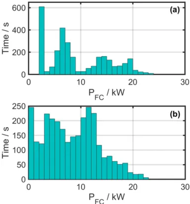
From Figure 10, it can be seen that active configuration manages to run the FC stack between PLow andPHigh regions. Operating the FC stack within this region results in higher efficiency
and less degradation of the system. Figure 10b shows that the passive configuration provides a homogeneous power distribution while it sometimes leads to the operation of the FC system in the low efficiency zone.
Figure 10: FC power distribution for a) active and b) passive coupling
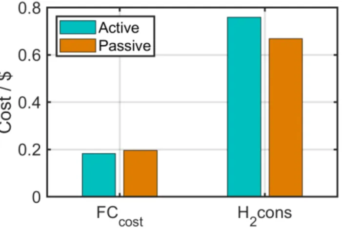
Figure 11 compares the cost of FC stack caused by the degradation as well as the hydrogen consumption for each considered case under the real driving profile condition. As explained earlier, the degradation cost of the FC stack is due to the idle time, number of start-stops, duration of heavy loading, and the operation time in high power condition. On the one hand, Figure 11 indicates that the FC degradation cost is $0.1825 and $0.1961 in active and passive configurations respectively. This result discloses the better performance of the active coupling by almost seven percent in terms of wear and tear in the FC system due to the management of the power between the sources while respecting their defined restrictions. On the other hand,
form Figure 11, it can be seen that the passive connection consumes less hydrogen than the active coupling by virtually 12 percent. This is essentially the result of not having the DC-DC converter electrical losses in the system.
Figure 11: Cost breakdown comparison of active and passive configuration To scrutinize deeper the pros and cons of having a passive coupling compared to the active one, a more detailed analysis from different perspectives is presented in Table 5.
Table 5: The cost comparison of FC-SC passive and active couplings
Type Active Passive
Trip cost $ 0.9420 $ 0.8650
No. Trips per tank 5.36 6.08
No. trips up to EOL of FC 5983 5569
Trip cost up to EOL $ 5636 $ 4817
Capital cost $ 3929 $ 2564
Total cost of the system $ 9565 $ 7381 Total system cost per hour $ 1.957 $ 1.623
According to this table, the trip cost, which is the sum of FC degradation and utilized
hydrogen, is less in passive configuration by 8%. Furthermore, the possible number of trips by one tank of hydrogen, calculated by using the total storage capacity of the tank and the
hydrogen consumption, is higher in the passive coupling by almost 13.5%. However, the possible number of trips before reaching the EOL of the FC stack is higher in the active coupling by practically 7%, which refers to the faster degradation of the stack in the passive configuration. This table also shows that the total cost of the system, which is composed of capital cost and trip cost up to EOL of the FC stack, is lower in the passive configuration by
22.8%. The last presented result in the table is related to the total cost of operating a passive or active configuration per hour, which is less in the passive coupling by 17%. This cost per hour has been obtained by the division of total cost by the number of hours the FC is able to operate before reaching its EOL. To sum up, Table 5 reveals that a passive coupling, despite of having a shorter operational time in the FC system, leads to a less expensive hourly total cost of the system.
5 Conclusions
This paper performs a comparative study of active and passive FC-SC couplings for the powertrain configuration of e-TESC 3W platform vehicle. In this respect, the size of the components is determined in relation to the requirements of the vehicle in the first place. Afterwards, the performance of the passive configuration is compared with a commonly used active one to spotlight the assets and liabilities of each case. An optimized FLC based on a real driving cycle of the e-TESC 3W platform is used to split the power between the FC stack and SC bank in the active configuration while the passive coupling does not require an EMS for power distribution. In order to investigate the performance of each configuration, an hourly total system cost for the operation of each case is calculated. This cost mainly contains the trip cost, which is composed of the FC degradation and consumed hydrogen costs, and the capital cost of the components. The performed analysis indicates that the hourly cost of the proposed passive connection is 17% less than the studied active configuration. It is worth reminding that the passive configuration causes higher rate of degradation in the FC system compared to the active one. However, this cost is compensated by the other aspects such as lower hydrogen consumption and the capital cost of the system.
Acknowledgements
This work was supported in part by Grant 950-230863 and 950-230672 from Canada
Research Chairs Program, and in part by Grant RGPIN-2018-06527 and RGPIN-2017-05924 from the Natural Sciences and Engineering Research Council of Canada.
List of Symbols
∆𝐹𝐶deg Voltage degradation of the FC stack / %
∆𝐹𝐶𝑎𝑑𝑑 Additional degradation of the FC / %
∆𝐹𝐶𝑛at Natural degradation of the FC / %
CO2 Oxygen concentration / mol cm-3
cp Air specific heat capacity / J K-1
CSC SC bank capacitance / F
CTrip Cost function / $
ENernst Cell reversible voltage / V
F Faraday constant / s A mol-1
Fair Resistance force against the air / N
Facc Accelerating force / N
Fenv Traction force resistance / N
Fgrade Grade related force / N
Froll Rolling resistance force / N
Ftr Traction force / N
g Gravity / m sec-2
Ggb Gearbox transmission ratio
Hcons Consumed Hydrogen / kg
Hfc Heat transfer coefficient / W K-1
idc/dc Converter current / A
IFC Current of the FC / A
iFC-sys Current of the FC system / A
iSC SC current / A
its Electric motor current / A
ktn Empirical coefficient
MCfc Thermal capacity of the FC / kJ K-1
MO2 Oxygen molar mass kg mol-1
Ncell Number of cells
ƞcomp Average compressor efficiency
ƞdc/dc Converter efficiency
ƞem Motor average efficiency / %
ƞgb Gearbox transmission efficiency / %
Ƞsys Efficiency of the FC system
ƞt Transmission efficiency / %
pamb Ambient pressure / Pa
pan Pressure in the anode / Pa
pca Pressure in the cathode / Pa
Pcomp Consumed power by the compressor / W
Pfan Consumed power by the FC fan / W
Pfc Generated power by the FC / W
pH2 Hydrogen partial pressure / Pa
PHigh FC high power limit / W
PLow FC low power limit / W
pO2 Oxygen partial pressure / Pa
Ptot Power at maximum acceleration / kW
Pts Transmission power / W
Qconv Convection heat transfer / W
qH2 Hydrogen flow / SLPM
Qheat Generated heat in the FC / W
rD Diode resistance / Ω
rSC SC bank resistance / Ω
Tamb Ambient temperatue / K
Tem Electric machine torque / N m
Tem_r Reference torque for electric machine / N m
Tfc Stack temperature / K
Uact Activation voltage drop / V
Ucon Concentration voltage drop / V
Ufc FC voltage / V
Uohmic Ohmic voltage drop / V
USC SC voltage / V
VEV vehicle speed / m s-1
Wair Rate of used air
WO2 Oxygen consumption rate
β Inverse of the limiting current / A-1
γ Ratio of specific heats of air
δ Mass factor
λ Oxygen excess ratio
ξn Parametric coefficients related to ohmic resistance
ρa Air density / kg m-3
ϒn Experiential coefficients related to activation loss
χO2 Oxygen mass fraction
Ωm Rotor rotation speed / rad s-1
𝑘n Degradation coefficient
References
[1] USDOE Energy Information Administration (EI), Washington, DC (United States). Office of Energy Analysis, 2019.
[2] Y. Wu, L. Zhang, Transportation Research Part D: Transport and Environment 2017, 51, 129-145.
[3] Z. P. Cano, D. Banham, S. Ye, A. Hintennach, J. Lu, M. Fowler, Z. Chen, Nature Energy 2018, 3, 279-289.
[4] B. Hollweck, M. Moullion, M. Christ, G. Kolls, J. Wind, Fuel Cells 2018, 18, 669-679.
[5] M. Bodner, A. Schenk, D. Salaberger, M. Rami, C. Hochenauer, V. Hacker, Fuel Cells
2017, 17, 18-26.
[6] F. X. Chen, Y. Yu, J. X. Chen, Fuel Cells 2017, 17, 671-681.
[7] D. Zhang, C. Cadet, N. Yousfi-Steiner, F. Druart, C. Bérenguer, Fuel Cells 2017, 17, 268-276.
[8] X. Zhang, Y. Yang, X. Zhang, L. Guo, H. Liu, Fuel Cells 2019, 19, 160-168. [9] T. Zimmermann, P. Keil, M. Hofmann, M. F. Horsche, S. Pichlmaier, A. Jossen,
Journal of Energy Storage 2016, 8, 78-90.
[10] R. C. Samsun, C. Krupp, S. Baltzer, B. Gnörich, R. Peters, D. Stolten, Energy Conversion and Management 2016, 127, 312-323.
[11] Q. Xun, Y. Liu, E. Holmberg, Proc. 2018 International Symposium on Power
Electronics, Electrical Drives, Automation and Motion (SPEEDAM), (Eds. A. Binder, A. Del Pizzo, I. Miki), Amalfi, Italy 2018, pp. 389-394.
[12] H. S. Das, C. W. Tan, A. H. M. Yatim, Renewable and Sustainable Energy Reviews
2017, 76, 268-291.
[13] J. P. Trovão, M. A. Silva, C. H. Antunes, M. R. Dubois, Applied Energy 2017, 205, 244-259.
[14] V. K. Kasimalla, N. S. G., V. Velisala, International Journal of Energy Research
2018, 42, 4263-4283.
[15] M. Kandi Dayeni, M. Soleymani, Clean Technologies and Environmental Policy
2016, 18, 1945-1960.
[16] R. E. Silva, F. Harel, S. Jemeï, R. Gouriveau, D. Hissel, L. Boulon, K. Agbossou, Fuel Cells 2014, 14, 894-905.
[17] C. Turpin, D. Van Laethem, B. Morin, O. Rallières, X. Roboam, O. Verdu, V. Chaudron, Mathematics and Computers in Simulation 2017, 131, 76-87. [18] H. Wang, A. Gaillard, D. Hissel, Renewable Energy 2019, 141, 124-138.
[19] S. Ait Hammou Taleb, D. Brown, J. Dillet, P. Guillemet, J. Mainka, O. Crosnier, C. Douard, L. Athouël, T. Brousse, O. Lottin, Fuel Cells 2018, 18, 299-305.
[20] K. Gérardin, S. Raël, C. Bonnet, D. Arora, F. Lapicque, Fuel Cells 2018, 18, 315-325. [21] B. Morin, D. Van Laethem, C. Turpin, O. Rallières, S. Astier, A. Jaafar, O. Verdu, M.
Plantevin, V. Chaudron, Fuel Cells 2014, 14, 500-507. [22] R. Shimoi, Y. Ono, WIPO, WO2005107360, 2005.
[23] D. Arora, K. Gérardin, S. Raël, C. Bonnet, F. Lapicque, Journal of Applied Electrochemistry 2018.
[24] 2.7V 650-3000F ultracapacitor, can be found under https://www.maxwell.com, 2013. [25] P. Pei, Q. Chang, T. Tang, International Journal of Hydrogen Energy 2008, 33,
3829-3836.
[26] H. Zhao, A. F. Burke, Fuel Cells 2010, 10, 879-896.
[27] B. Wu, M. A. Parkes, V. Yufit, L. De Benedetti, S. Veismann, C. Wirsching, F. Vesper, R. F. Martinez-Botas, A. J. Marquis, G. J. Offer, N. P. Brandon, International Journal of Hydrogen Energy 2014, 39, 7885-7896.
[28] J. P. F. Trovão, M. R. Dubois, M. Roux, E. Menard, A. Desrochers, Proc. 2015 IEEE Vehicle Power and Propulsion Conference (VPPC), Montreal, Quebec, 2015, pp. 1-6.
[29] J. P. F. Trovão, M. Roux, É. Ménard, M. R. Dubois, IEEE Transactions on Vehicular Technology 2017, 66, 5540-5550.
[30] A. S. Mohammadi, J. P. Trovão, M. R. Dubois, IET Electrical Systems in Transportation 2018, 8, 12-19.
[31] G. Wenzhong, IEEE Transactions on Vehicular Technology 2005, 54, 846-855. [32] R. Abousleiman, O. Rawashdeh, 2015 IEEE Transportation Electrification
Conference and Expo (ITEC), 2015, pp. 1-5.
[33] C. Mi, M. A. Masrur, Hybrid electric vehicles: principles and applications with practical perspectives, John Wiley & Sons, 2017.
[34] FCvelocity®-9SSL Product Manual and Integration Guide, can be found under www.ballard.com, 2017.
[35] V. Liso, M. P. Nielsen, S. K. Kær, H. H. Mortensen, International Journal of Hydrogen Energy 2014, 39, 8410-8420.
[36] C. H. Choi, S. Yu, I.-S. Han, B.-K. Kho, D.-G. Kang, H. Y. Lee, M.-S. Seo, J.-W. Kong, G. Kim, J.-W. Ahn, S.-K. Park, D.-W. Jang, J. H. Lee, M. Kim, International Journal of Hydrogen Energy 2016, 41, 3591-3599.
[37] Fuel Cell Technologies Office Multi-Year Research, Development, and
Demonstration Plan - Hydrogen Storage, can be found under www.energy.gov, 2015. [38] A. Bouscayrol, in Systemic Design Methodologies for Electrical Energy Systems (Ed.
X. Roboam), ISTE, 2012, pp. 89.
[39] L. Boulon, D. Hissel, A. Bouscayrol, M. Pera, IEEE Transactions on Industrial Electronics 2010, 57, 1882-1891.
[40] M. Kandidayeni, A. Macias, A. A. Amamou, L. Boulon, S. Kelouwani, Fuel Cells
2018, 18, 347-358.
[41] P. S. Oruganti, Q. Ahmed, D. Jung, Proc. WCX World Congress Experience, Michigan, U.S.A., 2018.
[42] X. Zhao, Y. Li, Z. Liu, Q. Li, W. Chen, International Journal of Hydrogen Energy
2015, 40, 3048-3056.
[43] J. M. Campbell, Gas conditioning and processing Volume 2: The Equipment modules, PetroSkills, U.S.A., 2014, pp. 197.
[44] L. Zubieta, R. Bonert, IEEE Transactions on Industry Applications 2000, 36, 199-205. [45] Y. Wang, S. J. Moura, S. G. Advani, A. K. Prasad, International Journal of Hydrogen
Energy 2019.
[46] Z. Hu, J. Li, L. Xu, Z. Song, C. Fang, M. Ouyang, G. Dou, G. Kou, Energy Conversion and Management 2016, 129, 108-121.
[47] K. Song, H. Chen, P. Wen, T. Zhang, B. Zhang, T. Zhang, Electrochimica Acta 2018, 292, 960-973.
[48] Fuel Cell Technologies Office Multi-Year Research, Development, and Demonstration Plan - Fuel Cells, can be found under www.energy.gov, 2015. [49] R. Zhang, J. Tao, IEEE Transactions on Fuzzy Systems 2018, 26, 1833-1843. [50] R. Zhang, J. Tao, H. Zhou, IEEE Transactions on Fuzzy Systems 2019, 27, 45-57. [51] Fuel Cell Technologies Office Multi-Year Research, Development, and
Demonstration Plan - Hydrogen Production, can be found under www.energy.gov,
2015.
[52] Z. Song, J. Li, J. Hou, H. Hofmann, M. Ouyang, J. Du, Energy 2018, 154, 433-441. [53] Electrical and Electronics Technical Team Roadmap, can be found under