ECSNeT++ : A simulator for distributed stream processing on edge and cloud environments

HAL Id: hal-02369500

https://hal.inria.fr/hal-02369500

Submitted on 19 Nov 2019

HAL is a multi-disciplinary open access

archive for the deposit and dissemination of

sci-entific research documents, whether they are

pub-lished or not. The documents may come from

L’archive ouverte pluridisciplinaire HAL, est

destinée au dépôt et à la diffusion de documents

scientifiques de niveau recherche, publiés ou non,

émanant des établissements d’enseignement et de

ECSNeT++ : A simulator for distributed stream

processing on edge and cloud environments

Gayashan Amarasinghe, Marcos Dias de Assuncao, Aaron Harwood, Shanika

Karunasekera

To cite this version:

Gayashan Amarasinghe, Marcos Dias de Assuncao, Aaron Harwood, Shanika Karunasekera.

EC-SNeT++ : A simulator for distributed stream processing on edge and cloud environments. Future

Gen-eration Computer Systems, Elsevier, In press, pp.1-18. �10.1016/j.future.2019.11.014�. �hal-02369500�

ECSNeT++ : A Simulator for Distributed Stream

Processing on Edge and Cloud Environments

Shanika Karunasekeraa

a_{School of Computing and Information Systems, The University of Melbourne, Australia} b_{Inria Avalon, LIP Laboratory, ENS Lyon, University of Lyon, France}

Abstract

The objective of Internet of Things (IoT) is ubiquitous computing. As a result many computing enabled, connected devices are deployed in various environ-ments, where these devices keep generating unbounded event streams related to the deployed environment. The common paradigm is to process these event streams at the cloud using the available Distributed Stream Processing (DSP) frameworks. However, with the emergence of Edge Computing, another con-venient computing paradigm has been presented for executing such applications. Edge computing introduces the concept of using the underutilised potential of a large number of computing enabled connected devices such as IoT, located out-side the cloud. In order to develop optimal strategies to utilise this vast number of potential resources, a realistic test bed is required. However, due to the over-whelming scale and heterogeneity of the edge computing device deployments, the amount of effort and investment required to set up such an environment is high. Therefore, a realistic simulation environment that can accurately predict the behaviour and performance of a large-scale, real deployment is extremely valuable. While the state-of-the-art simulation tools consider different aspects of executing applications on edge or cloud computing environments, we found that no simulator considers all the key characteristics to perform a realistic simulation of the execution of DSP applications on edge and cloud computing environments. To the best of our knowledge, the publicly available simulat-ors lack being verified against real world experimental measurements, i.e. for calibration and to obtain accurate estimates of e.g. latency and power consump-tion. In this paper, we present our ECSNeT++ simulation toolkit which has been verified using real world experimental measurements for executing DSP applications on edge and cloud computing environments. ECSNeT++ models deployment and processing of DSP applications on edge-cloud environments and

∗_{Corresponding author: School of Computing and Information Systems, The University of}

Melbourne, Victoria 3010, Australia.

Email addresses: gamarasinghe@student.unimelb.edu.au (Gayashan Amarasinghe), marcos.dias-de-assuncao@inria.fr (Marcos D. de Assun¸c˜ao), aharwood@unimelb.edu.au (Aaron Harwood), karus@unimelb.edu.au (Shanika Karunasekera)

is built on top of OMNeT++/INET. By using multiple configurations of two real DSP applications, we show that ECSNeT++ is able to model a real de-ployment, with proper calibration. We believe that with the public availability of ECSNeT++ as an open source framework, and the verified accuracy of our results, ECSNeT++ can be used effectively for predicting the behaviour and performance of DSP applications running on large scale, heterogeneous edge and cloud computing device deployments.

Keywords: Simulation, Edge Computing, Distributed Stream Processing, Internet of Things

1. Introduction

The recent surge of Internet of Things (IoT) has led to widespread introduc-tion and usage of smart apparatus in households and commercial environments. As a result the global IoT market is expected to hit$7.1 trillion in 2020 [1]. These smart devices have demonstrated to hold great potential to improve many sectors such as healthcare, energy, manufacturing, building construction, main-tenance, security, and transport [2][3][4][5]. For example, Trenitalia, the main Italian train service operator is currently using an IoT based monitoring system to move from a reactive maintenance model to a passive maintenance model to deliver a more reliable service to travellers [6].

One common trait of many IoT deployments is that the devices monitor the environment they are deployed in, and produce events related to the current status of the said environment. This generates a time series of events that can be processed to extract vital information about the environment. Generally this event stream is unbounded and hence, Distributed Stream Processing (DSP) techniques can be utilised in order to process the events in real-time [7].

Apache Storm[8], Twitter Heron[9], Apache Flink[10] are modern DSP frame-works widely used for distributed stream processing. Cloud computing has be-come the main infrastructure for deploying these frameworks, where they are generally hosted by large-scale clusters offering enormous processing capabilit-ies and whose resources are accessed on demand under a pay-as-you-go business model.

As mentioned earlier, with the involvement of IoT, the sources where events are generated are located outside the cloud. Therefore, if we are to process these event streams using DSP frameworks, the current status quo is to generate data streams at the IoT devices and transmit them to the cloud for processing [7]. However, this arrangement is not ideal due to the higher latency caused by the communication overhead between these IoT devices and the cloud, which often becomes the bottleneck [11][12].

On the other hand, Edge computing is emerging as a potential computing paradigm that can be utilised for sharing the workloads with the cloud for suit-able applications [13][14]. The goal of edge computing is to bring processing closer to the end users or in proximity to the data sources [12][15]. As a res-ult, concepts such as cloudlets, Mobile Edge Computing, and Fog Computing,

are utilised where the processing is conducted at the base stations of mobile networks or servers that reside at the edge of the networking infrastructure, sometimes even referred as the Edge Cloud [15]. However, with the advance-ments in processing and networking technologies, processing should not be lim-ited only to these processing servers that are at the edge of the networking infrastructure. Therefore, we utilise a broad definition for Edge Computing as computations executed on any processing element located logically outside the cloud layer which includes either edge servers and/or clients [12][15][16][17][18]. These devices are located closer to the data sources, sometimes acting as data sources or thick clients themselves. Wearable devices, mobile phones, personal computers, single board computers, many common smart peripherals with com-putational capabilities (such as many IoT devices), mobile base stations, and networking devices with processing capabilities belong to this category. With the increasing computational power of mobile processors, we believe these edge devices that are located closer to the end users, have potential that is not being fully utilised [19].

The commercial interest in the utilisation of IoT technologies for processing data at the edge, is shown with the invention of Google’s implementation of ar-tificial intelligence at the edge [18], in-device video analysis devices [20][21][22], home automation devices [23], and industrial automation applications [24]. However, these edge devices have limitations of their own as well – such as being powered by batteries and being connected to the cloud with limited bandwidth networks, which are often wireless.

The number of Edge computing devices (including IoT devices) is increasing exponentially. These devices have heterogeneous specifications and character-istics which cannot be generalised in a trivial manner. Many of these devices have potential that can be utilised in many ways. Therefore, finding efficient ways to utilise these heterogeneous resources is important and a timely require-ment. However, creating a real test environment for running such experiments is challenging due to the amount of effort and investment required. As a result, simulation has become a suitable tool that can be used to run these experiments and to acquire realistic results [25][26].

Currently, to the best of our knowledge, there is no complete simulation environment that provides both an accurate processing model and a network-ing model for edge computnetwork-ing applications – specifically for distributed stream

processing application scenarios. The available simulation tools lack an

ac-curate network communication model [25][26]. However, on edge computing applications, the network communication plays a critical role mainly due to the bandwidth and power limitations [13][26]. In addition, none of the available simulation tools have been verified against a real device deployment which we believe is equally important since simulation without a sense of accuracy and reliability of the acquired results is ineffective.

As a solution, we have implemented a simulation toolkit, ECSNeT++, with an accurate computational model for executing DSP applications, on top of the widely used accurate network modelling capabilities of OMNeT++. OMNeT++ is one of the widely used network simulators due to its in-detail network

mod-elling and accuracy [26][27]. We have verified ECSNeT++ against a real device deployment to ensure that it can be properly calibrated to acquire realistic measurements compared to a real environment.

More specifically, we make the following contributions:

• We present an extensible simulation toolkit, which we call ECSNeT++, built on top of the widely used OMNeT++ simulator that is able to simu-late the execution of DSP application topologies on various edge and cloud configurations to acquire the end to end delay, processing delay, network delay, and per-event energy consumption measurements.

• We demonstrate the effectiveness and adaptability of our simulation toolkit by simulating multiple configurations of two realistic DSP applications from the RIoTBench suite [28] on edge-cloud environments.

• We verify our simulation toolkit against a real edge and cloud deployment with multiple configurations of the two DSP applications to show that the measurements acquired by simulations can closely represent real-world scenarios with proper calibration.

• We display the extensibility of our simulation toolkit by adopting the LTE network capability from the SimuLTE framework [29] to simulate a realistic DSP application on an LTE network.

• We have made our simulation toolkit1 _{and the LTE plugin}2_{, open source}

and publicly available for use and further extension.

A high-level comparison of the features of ECSNeT++ against the state-of-the-art simulators publicly available as shown in Table 1, indicates that EC-SNeT++ is the only simulation tool of its kind for simulating the execution of DSP applications on edge and cloud computing environments that has also been verified against a real experimental set-up to demonstrate its capabilities.

Table 1: Comparison of ECSNeT++ simulation toolkit against state-of-the-art

Feature CloudSim EdgeCloudSim OMNeT++ iFogSim ECSNeT++

[30] [26] [27] [25] toolkit

Edge Devices × X × X X

Cloud Server X X × X X

Realistic Network Model Limited X X Limited X

Power Model X × X X X

Processing Model X X × X X

Device Mobility × X X × X

Comprehensive DSP Task Model × × × Limited X

DSP Task Placement × × × X X

Verification against real set-up × × × × X

The rest of this paper is organised as follows. We provide a brief background about the characteristics of host networks and DSP applications in Section 2,

1_{Available at https://sedgecloud.github.io/ECSNeTpp/}

whereas the modelling and simulation tool is described in Section 3. The eval-uation scenario and performance results are presented in Section 4 followed by the in detail analysis of lessons learnt during our study in Section 5. Section 6 discusses related work and Section 7 concludes the paper.

2. Background

2.1. Characteristics of a Host Network

An execution environment (i.e. a host network) is a connected graph where vertices represent devices and the edges of the graph are the network connectiv-ity. In our study we consider an environment that consists of cloud servers and edge computing devices, where the edge devices are connected to the cloud through a LAN and WAN infrastructure.

Each host device has data processing characteristics (with respect to the available CPU and the associated instruction set), network communication char-acteristics (via NICs and network protocols), and data storage charchar-acteristics (volatile and non-volatile storage). The network itself has a topology, different network components such as routers, switches and access points, and quantifi-able characteristics such as the network latency, bandwidth and throughput.

The processing power and storage characteristics vary depending on the host device. A cloud node usually provides a virtual execution environment often with high processing power with multi-core multi-threaded CPUs, and high RAM capacity and speed. In contrast, an edge device has lower processing power and memory. For an example a Raspberry Pi 3 Model B device has a 4 core CPU with 1024MB memory, while a high-end mobile phone may have a quad/octa-core CPU with 6/8GB memory. In addition, these different devices may have their own instruction sets depending on the processor architecture. All of these processing characteristics and memory characteristics are generally available with the device specifications.

The most power consuming components of these host devices are the network subsystem and the processing unit. The power consumption characteristics of hosts for the most part depend on the underlying hardware. The cloud servers consume significant amount of power since they have unconstrained access to power. On the other hand, the edge devices are constrained by power avail-ability. However, in most of these devices, it is possible to monitor and profile the power consumption characteristics empirically [31] or acquire them from the device specifications.

The characteristics of the underlying network depend on the network topo-logy and the components of the network. A Local Area Network has higher bandwidth and throughput with lower latency but a smaller, less intricate to-pology. A Wide Area Network has a more complex topology but often with higher latency that increases with distance. Depending on the location of the edge devices and cloud servers, a combination of LAN and WAN may be utilised to build the host network.

2.2. Characteristics of a DSP Application

As illustrated in Figure 1, a DSP application consists of four components, source, operator, sink, and the dataflow. In any DSP application, the sinks, sources and operators, known as tasks, are placed and executed on a processing node. These different tasks in the application topology have their own charac-teristics depending on the application.

r events/s σr events/s m kB selectivity ⍴m kB ratio : σ productivity ratio : ⍴ event generation rate : r ev/s event size : m kB

Source Operator Sink

Task Dataflow Event

Figure 1: Components and characteristics of a DSP application where a source generates events, which are then processed by the operators down stream, and reach a sink for final processing. Each source governs the event generation rate and the size of each event generated. Each operator manipulates either the properties of each event, the event processing rate or both.

A source generates events – therefore has an event generation rate and an event size associated with it. The event generation rate vary from one applic-ation to another. We can expect a uniform rate if the source is periodically reading a sensor and transmitting that value to the application. If the source is configured to read a sensor and report only if there is a change in reading, it can produce events at a rate that is difficult to predict. If the source is related to human behaviour, e.g.: activity data from a fitness tracker, the event gener-ation rate can follow a bimodal distribution with local maxima, where people are most active in the morning and the evening [28].

Each generated event has a fixed or variable size depending on the applic-ation. If the event is generated by reading a specific sensor, often an upper bound for the event size is known due to the known structure of an event. For example, a temperature reading from a thermometer may contain a timestamp, sensor ID, and the temperature reading. Therefore, the size of such an event can be trivially estimated. However, if each event is a complex data structure such as a twitter stream, which can contain textual data and other media, then the event size may vary accordingly.

For a given operator, two characteristics control the dataflow. For an op-erator Tj, the selectivity ratio σTj is the ratio between the outgoing

through-put λout

Tj and the ingress throughput λ

in Tj [32][28], i.e. σTj = λ out Tj /λ in Tj. We

also introduce, for an operator Tj, productivity ratio ρTj, which is the ratio

between an outgoing message size βout

Tj and the incoming message size β

in Tj, i.e. ρTj = β out Tj /β in

Tj. The distribution of the selectivity and productivity ratios

op-erator [28]. For example, if the opop-erator is calculating the average of incoming temperature readings for a given time window, an upper bound for the pro-ductivity ratio can be estimated since outgoing event structure is known. If the window length is known, the selectivity ratio can also be estimated. However, if the operator is tokenizing a sentence in a textual file, the productivity ratio and the selectivity ratio for that particular operator can vary depending on the input event. By profiling each operator, the selectivity and productivity ratio distribution can be estimated to a certain extent. But this is highly application dependent.

3. ECSNeT++ Simulation Toolkit

ECSNeT++ is a toolkit that we designed and implemented to simulate the execution of a DSP application on a distributed cloud and edge host

en-vironment. The toolkit was implemented on top of the OMNeT++

frame-work3_{[27] using the native network simulation capabilities of the INET}

frame-work4_{. OMNeT++ framework has matured since its inception in 1997 with}

frequent releases5_{. In addition to the maturity, and widespread use among the}

scientific community[33][34], OMNeT++ enabled the development of a modular, component based toolkit to simulate the inherent characteristics of edge-cloud streaming applications and networks.

The high-level architecture of ECSNeT++ is illustrated in Figure 2. We implemented the host device model, and the power and energy model by ex-tending the INET framework. The multi-core multi-threaded processing model is built on top of our host device model. The components of the DSP application model use all these features to simulate the execution of an application on an Edge-Cloud environment. The following subsections describe in detail how the different elements of a stream processing solution are modelled in the simulation toolkit. In Table 2 we summarize the symbols used throughout this paper. 3.1. Host Network and Processing Nodes

We have implemented a set of processing nodes of two categories: cloud nodes and edge nodes. As mentioned earlier, the edge computing nodes are the leaf nodes that are connected to the network via an either a IEEE 802.11 WLAN using access points for each separate network or via an LTE Radio Access Network with the use of ECSNeT++ LTE Plugin and eNodeB base sta-tions. Depending on the scalability of the edge layer, the number of access points or base stations can be configured. They act as the bridge between the edge clients and the wired local area network (See Figure 4 and Figure 17). All the wired connections are simulated in this host network as full duplex Eth-ernet links. However, by utilising the INET framework with our host device

3_{https://omnetpp.org/} 4_{https://inet.omnetpp.org/}

Figure 2: High level architecture of ECSNeT++ which is built on top of the OMNeT++ simulator and the INET framework

implementations, it is possible to simulate a complex LAN and WAN configur-ation as required. In addition, the use of an LTE network for communicconfigur-ation between the edge and the cloud by using the SimuLTE simulation tool6and the ECSNeT++ LTE Plugin, which provides a LTE network connectivity model, shows the extensibility of the networking model available in ECSNeT++.

We have implemented each type of edge device that use IEEE 802.11 con-nectivity by extending the WirelessHost module of INET framework which simulates IEEE 802.11 network interface controllers for communication. For LTE connected edge devices, each device is a standalone module with a LTE enabled network interface controller which implements the ILteNic interface from the SimuLTE tool. A cloud node is implemented by extending the Stand-ardHost module of the INET framework. This grants the cloud nodes the ability to connect to other modules (switches, routers, etc.) via a full-duplex Ethernet interface.

Each host has the capability to use either TCP or UDP transport for commu-nication. The preferred protocol can be configured by enabling the <host>.hasTcp or <host>.hasUdp property and setting the <host>.tcpType or <host>.udpType property appropriately on the omnetpp.ini file (or the relevant simulation

Table 2: Symbols used in the model Symbol Description Ti Task i Opi Operator i Soi Source i Sii Sink i

Vj Edge device or Cloud server j

σTi Selectivity ratio of Ti

ρTi Productivity ration of Ti

rSoi Event generation rate of Soi

mSoi Generated event size of Soi

δTiVj Processing time per event, per-task Ti, per-device Vj

ζTiVj CPU cycles consumed per event, per-task, per-device

CVj Per core processing frequency of device Vj

ηVj Number of CPU cores on device Vj

ψVj Number of threads per CPU core on device Vj

Φtotal Total power consumption

Φidle Idle power consumption

Φcpu(u) CPU power consumption at utilisation u

Φwif i,idle WiFi idle power consumption

Φwif i,up WiFi transmitting power consumption

Φwif i,down WiFi receiving power consumption

figuration file) to use the TCP or UDP protocol for communication. 3.2. DSP Application

Three separate task modules were developed to represent namely sources, op-erators, and sinks. A StreamingSource task module produces events depending on the configurations for event generation and event size. A StreamingOper-ator task module accepts incoming events, processes them using the processing model of the host and sends them to the next task or tasks according to the DSP topology. A StreamingSink task module is the final destination for all incoming events.

Each of these task modules should be placed on a host device with processing capabilities and can be connected according to the adjacency matrix of the DSP topology, which needs to be provided to the simulator, to simulate the dataflow of a DSP application. Instances of these modules should be configured, depending on the characteristics of each task in the DSP application topology. The processing of events in each of these tasks shall be done according to the processing model we have implemented in the simulation toolkit.

3.2.1. Placement Plan

The placement plan, which dictates the placement of one or more DSP ap-plication topology tasks (Sources, Operators and Sinks) on to the host networks,

needs to be generated externally depending on the requirements of the applic-ation deployment and should be submitted to ECSNeT++. For example, the placement plan contains a mapping for each task in the DSP application topo-logy to a host device(or devices) along with other characteristics relevant to the task if it is executed on the particular host device(or devices). Therefore, along with the placement of the topology, every attribute related to each task, e.g. the processing delay of each task, event generation rate and generated message size of a source, selectivity and productivity distribution of an operator, need to be configured in the placement plan itself. We have implemented an XML schema to define the placement plans. We have decoupled the placement plan generation from the ECSNeT++ to allow the users to use any external tool to generate placement plans and to produce an XML representation of the plan using our schema.

3.2.2. Source

StreamingSource module represents a streaming source in the topology. Responsibility of each StreamingSource module is to generate events as per the configuration and to send the generated events downstream to the rest of the application topology. Two attributes affect the event stream generated at any given source in the topology; the generated event size and the distribution of the event generation rate. These attributes can be configured in the Stream-ingSource module. Once configured, the StreamStream-ingSource module starts gen-erating events as per the message size and event rate distributions and sends the generated events to the adjacent tasks.

The generated event size depends on the type of the application topology. A developer can simulate this characteristic by implementing the ISourceMes-sageSizeDistribution interface and configuring the placement plan by assign-ing the characteristic to the respective source such as a uniformly distributed message size distribution. Similarly the ISourceEventRateDistribution in-terface can be implemented, followed by an appropriate configuration in the placement plan, to incorporate different event generation rates for each source in the topology such as a bimodal event generation rate distribution.

Once these characteristics are configured for each source, they will produce events accordingly, that can be processed by operators connected to the data flow.

3.2.3. Operator

An operator in a topology can be simulated by configuring and placing a StreamingOperator module. The responsibility of each operator is to process any and all incoming streaming events and to produce one or more resulting events based on the characteristics that define its function; the selectivity ra-tio and the productivity rara-tio. By implementing the IOperatorSelectivity-Distribution interface, the selectivity ratio distribution of each operator can be simulated. Similarly the IOperatorProductivityDistribution interface should be implemented to simulate the productivity ratio distribution of a re-spective operator. Each of these implementations needs to be configured with

appropriate parameters according to the application topology in the placement plan. The parameter values can be acquired by profiling the incoming and outgoing events of each operator or by analysing the topology.

When an event arrives at an operator, the operator changes the outgoing event size and the outgoing event rate based on the productivity distribution and the selectivity distribution of that operator, and emits a corresponding event (or events) which are sent to the next operator or sink according to the application topology (denoted by the adjacency matrix in the simulator). 3.2.4. Sink

We have implemented the StreamingSink module to simulate the functions of a sink in the topology. Each sink acts as the final destination for all the arriving events and emits the processing delay, network delay, and the total latency of each event.

Apart from the above configurations, for each of these sources, operators, and sinks, the attributes to calculate processing delay needs to be configured. The following subsection describes how the processing model has been imple-mented and how to configure this model appropriately for each task in the DSP application topology being simulated.

3.3. Processing Model

Each processing node in the host network has a processing module to simu-late a multi-core, multi-threaded CPU. The processing of an event is simusimu-lated by holding the event in a queue for a time period δTiVj.

Each processing node shall be configured with 3 parameters; number of CPU cores ηVj, frequency of a single CPU core CVj, and the number of threads per

core ψVj. The CPUCore module of ECSNeT++ is implemented to simulate a

single CPU core instance. Each host device has CPUCore module instances equal to the number of CPU cores in that particular host as configured.

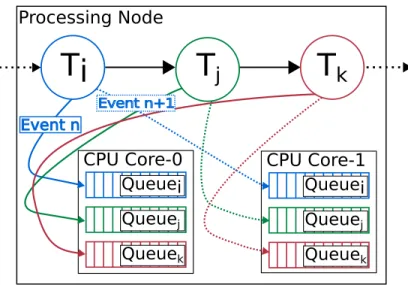
Figure 3 shows the processing of an event at a processing node. Since each processing node has tasks placed on it according to the placement plan as de-scribed earlier in Section 3.2.1, when an event arrives at a particular task, the task selects a CPU core for processing depending on the scheduling policy. We implemented a Round-robin scheduler for this study. However, it is possible to extend this behaviour to introduce other scheduling policies to the processing model by implementing the ICpuCoreScheduler interface. Once a CPU core is selected, the task sends the event to that core for processing. A CPU core maintains an exclusive non-priority FIFO queue for each operator, simulating the behaviour of a multi-threaded execution where the execution of each task is done in a single thread which depicts a thread per task architecture.

There exist two methods to acquire the per event processing delay for a task running on a particular device (δTiVj). Each task can be configured in

the placement plan to directly provide per event processing time which can be measured by profiling the running time of a task per event. If this is not feasible, the number of CPU cycles required to process the particular event in

Processing Node

Ti

T

_j

T

_k

CPU Core-0

Queuei

Queue

Queue

CPU Core-1

Queuei

Queue

Queue

Figure 3: A processing node (Va) with a dual core CPU and 3 DSP tasks (Ti, Tj, Tk) assigned

to it, processes an incoming event n by sending the event to a selected CPU core in round-robin manner. Each CPU core maintains an exclusive non-priority queue for each task. Each queue holds an unprocessed event for a time period δTiVa and releases the event back to the task

that sent the event to that particular CPU core. This concludes processing of the particular event by the said task.

the particular CPU architecture can be determined empirically by profiling an operator[35] or even by analysing the compiled assembly code, depending on the complexity of the application code, which in turn can be used to calculate the per event processing time.

In our experiments we use per event processing time directly since it can be measured from our real experiments.

After holding the event in the queue for the processing delay acquired by either of the above mentioned methods, the CPU core removes the event from the queue, and sends it back to the task that sent it, which completes the processing of the particular event on that task.

When a source has generated an event or an operator receives a processed event, it sends the event to the next operator or sink downstream. Each event is processed in this manner until it reaches a sink. This processing model is used by all the sources, operators, and sinks in the configured DSP application during the simulation.

3.4. Power and Energy Model

In ECSNeT++ we have implemented two power consumption characteristics for the edge devices connected via the IEEE 802.11 WLAN. The network power consumption measures the amount of power consumed while receiving and/or transmitting a processed event. The processing power consumption measures the amount of power consumed while processing a particular event at a CPU

core. In addition, the idle power consumption measures the amount of power consumed by the device while idling.

We have implemented and configured the NetworkPowerConsumer class to simulate the power consumption of the network communication over IEEE 802.11 radio medium. Each processing node in the edge layer has an instance of a NetworkPowerConsumer assigned to it. When the state of the radio changes, the consumer calculates the amount of power that would be used by that state change and emits that value. The NetworkPowerConsumer class has to be con-figured with idle power consumption of the device without any load, idle power consumption of the network interface, transmitting power consumption of the network interface, and the receiving power consumption of the network interface. These values can be measured or estimated based on empirical data [31][36]. The power consumption is determined, depending on the radio mode, the state of the transmitter, and the state of the receiver.

We have implemented and configured the CPUPowerConsumer class on EC-SNeT++ to simulate the power consumed by the processor in each edge based processing node. With our processing model, a CPU core operates within two states, CPU idle state and the busy state. When the CPU core is processing an incoming event, as per Section 3.3, it operates in the busy state and otherwise in an idle state. When a CPU core changes its state, the CPUPowerConsumer calculates the amount of power associated with the relevant state change. The CPUPowerConsumer is configured using the power consumption rate with respect to its utilisation which can be measured or estimated [31][36].

When a power consumption change is broadcast by a consumer, the Ideal-NodeEnergyStorage module calculates the amount of energy consumed during the relevant time period by integrating the power consumption change over the time period and records that value. However, it is important to note that the IdealNodeEnergyStorage does not have properties such as memory effect, self-discharge, and temperature dependence that can be observed on a real power storage.

The total power Φtotalconsumed at each edge device can be calculated by the

following Equation (1) [31][36]. The total power consumption is estimated by summing the power consumption of individual components as configured. Here Φidle is the idle power consumption without any load on the system, Φcpu(u)

is the power consumed by CPU when the utilisation is u%, and Φwif i,up(r)

and Φwif i,dn(r) represent the power consumed by the network interface for

transmitting and receiving packets over the IEEE 802.11 WLAN at the data rate of r.

Φtotal=Φidle+ Φcpu(u) + Φwif i,idle+ Φwif i,up(r) + Φwif i,dn(r) (1)

The components of this approximation function can be calibrated in the simulation configuration by either measuring the individual power consumption components of the device(s) or by referring to power characteristics specifica-tions of the device(s). Both uplink and downlink energy consumption should be

Table 3: Specification of host devices used in experimental set-up

Edge Cloud

Proc. Architecture ARMv7 x86 64

Processor Freq. 1.2GHz 2.6GHz

CPU Cores 4 24

considered since as per our state based power model and the duplex nature of packet transmission, arrival or the departure of a packet at the relevant network interface, triggers the energy consumed for that state change at the network in-terface to be recorded. All such recorded state changes are accumulated to produce the total power and energy consumption for the simulation.

At this stage of our study, we are only interested in the power/energy con-sumption of the edge devices. Therefore, we have limited the power concon-sumption simulation to only the edge devices, and the wireless network communication between the edge devices and the access points. However, due to the modu-lar architecture of the ECSNeT++, the power model can be extended to other processing nodes and communication media such as the LTE RAN as well.

4. Experiments and Evaluation

We use two set-ups for experiments. To run the ECSNeT++ simulator

in headless mode we use a m2.xlarge instance, which consists of 12 VCPUs,

48GB RAM, and a 30GB primary disk on the Nectar cloud7_{. We execute}

the simulation of ETL and STATS application topologies on this set-up with different operator allocation plans, and acquire the relevant measurements.

In order to verify the IEEE 802.11 WLAN based simulations of ECSNeT++ simulator against a real-world experimental set-up, we have established a simple experimental set-up using 2 Raspberry Pi 3 Model B (edge) devices which con-nect to two access points to create 2 separate edge sites. The access points are then connected to a router which connects to a single cloud node (cloud). The cloud node has the processing power of 24 core Intel(R) Xeon(R) CPU E5-2620 v2 at 2.60GHz and 64GB of memory. This selected host network for the real experiment set-up is shown in Figure 4 and the configurations are available in Table 3. The clocks of all these host devices are synchronized using the Network Time Protocol. All the communications between the edge and the cloud occur over the TCP protocol.

We have implemented the DSP applications using Apache Edgent8

frame-work which runs on Java version 1.8.0 65 on each edge device and cloud server in the experimental set-up. Apache Edgent is a programming model and a mi-cro kernel which provides a lightweight stream processing framework that can be embedded in many platforms.

7_{https://nectar.org.au/research-cloud/} 8_{http://edgent.apache.org/}

stargazer-3 cloud node

Router 1

Access Point 1

Edge device 1 Raspberry Pi 3 Model B node

PWR OK LKN FDX 10M Raspb erry P i Access Point 2 Edge device 2 Raspberry Pi 3 Model B node

PWR OK LKN FDX 10M Raspb erry P i

Figure 4: Simple experimental set-up used for simulator calibration and verification

4.1. Application Topologies and Allocation Plans

We use a simplified version of the ETL application topology and the STATS application topology from the RIoTBench suite [28] as the DSP applications for the experiments. The ETL application has a linear topology (See Figure 5) which extracts information from a given CSV file and converts the information to SenML format after preprocessing. The STATS application has a diamond topology (See Figure 6) which extracts information from a given CSV file and runs a statistical analysis of the information to produce a set of line plots. These topologies can be executed on either, edge, cloud or both.

SenML Parser

Range Filter

Bloom

Filter Interpo-_lation Join Annotate

CsvTo SenML Sink 1 Source σ = 5 ρ = 0.33 σ = 1 ρ = 1 σ = 1 ρ = 1 σ = 1 ρ = 1 σ = 0.2 ρ = 1.3 σ = 1 ρ = 1 σ = 1ρ = 2

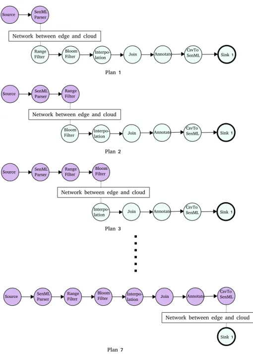
Figure 5: Simplified ETL Application Topology from the RIoTBench suite We have partitioned the ETL application topology into two partitions in 7 ways as illustrated in Figure 7 where one partition is placed on the edge device (purple nodes) and the other partition is placed on a cloud server (blue nodes). The two partitions communicate using the communication media as configured. Then we execute the application on both the real world set-up and the simulator to process a fixed number of events, and acquire delay and

Source SenML Parser Linear Regr. Block Window Ave Distinct Approx. Count Multi Line Plot Sink σ = 5 ρ = 0.33 σ ρ σ ρ σ ρ σ ρ = 1 = 2 = 1 = 1 = 1 = 1 = 0.04 = 0.0025

Figure 6: Simplified STATS Application Topology from the RIoTBench suite

Table 4: Characteristics of the operators of the ETL and STAS applications used in the experiments

Application Operator(s)

Name Selectivity Productivity

ETL SenML Parser 5 0.33

Range Filter 1 1 Bloom Filter 1 1 Interpolation 1 1 Join 0.2 1.3 Annotate 1 1 Csv To SenML 1 2

STATS SenML Parser 5 0.33

Linear Regression 1 2

Block Window Average 1 1

Distinct Approx. Count 1 1

Multi Line Plot 0.04 0.0025

edge energy consumption measurements. Similarly, we have partitioned the STATS application topology into two partitions in 6 ways where one partition is placed on the edge and the other is placed on the cloud. Then we execute each placement plan on both the simulator and the real experiment set-up. For each plan, we also vary the source event generation rate while keeping other parameters constant.

4.2. Measurements

In order to evaluate the applications, we are using four measurements – processing delay per event, network transmission delay per event, total delay per event, and average power consumption at each edge device. These measure-ments can be collected for each DSP application executed on each host network, and can be used to monitor the performance of each application on either the simulation or the real experiment.

4.2.1. Delay Measurements

Each individual operator in the DSP application topology appends the cessing time taken for a particular event and the sum of these individual pro-cessing times is recorded as the per event propro-cessing time for each event. When

SenML Parser

Range Filter

Bloom

Filter Interpo-lation Join

Source

Annotate CsvTo_SenML Sink 1

Plan 1 Network between edge and cloud

SenML Parser

Range Filter

Bloom

Filter Interpo-_lation Join

Source

Annotate CsvTo_SenML Sink 1

Plan 2 Network between edge and cloud

SenML Parser Range Filter Bloom Filter Interpo-lation Join Source

Annotate CsvToSenML Sink 1

Plan 3 Network between edge and cloud

SenML Parser

Range Filter

Bloom

Filter Interpo-lation Join

Source Annotate

CsvTo SenML

Sink 1

Plan 7

Network between edge and cloud

Figure 7: Possible placement plans for the Simplified ETL Application Topology - purple nodes are placed on the edge while blue nodes are placed on the cloud

a network transmission occurs, the network transmission time for each particu-lar event is recorded as well. The total delay per event is defined as the sum of

individual processing delays and network transmission delays of the particular event. The same approach is used in both the simulation and the empirical set-up.

4.2.2. Power and Energy Measurements

To have a more clear estimate on the power consumed by edge equipment in the experiment set-up, we designed a power meter and a set of scripts to measure the power consumed by our Raspberry Pi device while the DSP application is being executed.

ADC 2

ADC 1

Data

collection

Raspberry

Pi 3

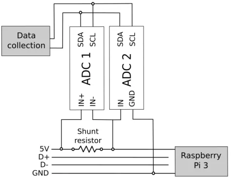
Figure 8: The power measurement set-up for the Raspberry Pi 3 device. ADC 1 and 2 are used to measure the voltage across the shunt resistor and the input voltage respectively. Data collection scripts record the power consumption periodically, using the voltage and current measurements.

Raspberry Pi’s are devices that can be powered via USB. The power con-sumption is hence measured by inserting a shunt resistor in the 5V USB line as depicted in Figure 8. The resistor causes a voltage drop that is proportional to the current drawn by the Raspberry Pi. An Analog to Digital Converter (ADC) is used to measure the voltage across the resistor (i.e. ADC 1) in order to compute the amount of current drawn by the Pi, whereas ADC 2 measures the input voltage used to compute the power. ADC 1 and 2 are respectively an ADC Differential Pi and and ADC Pi Plus, both produced by AB Electronics

Table 5: Network configuration used in both the real device deployment and the simulation.

Property Value

WLAN operation mode IEEE 802.11b

WLAN Bit rate 11 Mbps

WLAN frequency 2.4 GHz

WLAN radio bandwidth 20 MHz

WLAN MTU 1500 B

WLAN transmission queue length 1000

WLAN RTS threshold 3000 B

WLAN MAC retry limit 7

WLAN Transmission power 31 dBm

Ethernet Bit rate 1 Gbps

UK9. Both ADCs are based on Microchip MCP3422/3/4 that enable a

resolu-tion of up to 18 bits. Data collecresolu-tion scripts are executed by another Raspberry Pi device in the environment10_.

Prior to each configuration (i.e. placement plan) of the ETL or STATS application is executed on the experimental set-up (Figure 4), the data collec-tion scripts are executed in order to measure the power consumpcollec-tion of the edge device periodically. Measured power consumption values are used to cal-culate the average power consumption by the edge device in each experiment afterwards.

In ECSNeT++, we use the power and energy model as described in Sec-tion 3.4 to record the total energy consumpSec-tion for each execuSec-tion of the different configurations of the application and calculate the average power consumption for the respective time period.

4.3. Calibrating the Simulator

In this section we describe how the simulator has been calibrated in order to accurately simulate the real world experiments for the ETL application.

The WLAN between the edge node and the access point has a limited band-width of 11Mbps and operates in IEEE 802.11b mode. The rest of the Full duplex Ethernet network operates at 1Gbps bandwidth. The host network con-figurations as described in Table 5 are mirrored in the host concon-figurations of the simulator and the experimental set-up. For the power consumption measure-ments, we have acquired the values illustrated in Table 6 on the experimental set-up and we have configured ECSNeT++ using the same values. For all the other parameters, we use the default configuration values in OMNeT++.

First, each task in each application is profiled to measure the per event processing time (in nano second precision) for each CPU architecture. These measured values are used as the per event processing time, δTiVj value in each

9_{https://www.abelectronics.co.uk}

Table 6: Measured average power consumption values for Raspberry Pi 3 Model B used in the simulation. See Equation (1) for usage of these values.

Property Value (W) Φidle 1.354 Φcpu(100%) 0.258 Φcpu(400%) 0.955 Φwif i,idle 0.118 Φwif i,up 0.175 Φwif i,dn 0.132

placement plan. Then the network transmission delay between edge and cloud is measured for each case and these measured delay distributions are used for the configuration of delays in the simulator for each plan. While the event generation rate is varied, the initial event size of the source, and selectivity and productivity ratios of the operators are measured in the real application and the same values are used in the simulation set-up. Each application is executed until 10000 events are processed, and the experiments are concluded once the measurements are acquired for each of these processed events in both the simulator and the experimental set-up.

4.4. Evaluation of Delays

Figure 9 and Figure 10 show all the delay measurements for fixed source event generation rate of 10 events per second and 100 events per second respectively for all the considered placement plans of ETL application (Figure 7). Similarly, Figure 11, and Figure 12 shows the delay measurements of all the placement plans of STATS app running at 5 and 10 events per second. Each experiment is concluded when 10000 events have been processed. We conduct a qualitative analysis of the observed results for each scenario.

4.4.1. Network Delay

We first evaluate the network delay parameter for each scenario. In Figure 9 and Figure 10 the network latency values follow the same trend even though the real experimental set-up shows higher interquartile range with respect to the simulation set-up, where the variations in the simulated values are limited. In the experiments, we calculate the network delay as the time taken by an event to leave an edge device and arrive at the cloud server, which includes all the latencies caused by the management of packet delivery over the communication channel such as CSMA/CA, rate control, packet retransmission and packet or-dering caused by failures, etc., which results in the variations we observe in the results. It is not possible to simulate an identical environment since it is not possible to measure these intricacies. Since the IEEE 802.11 implementation of OMNeT++/INET has the same characteristics and due to the close calibration of the simulator (Section 4.3) we can observe some variation in the network delay measurements of the simulation specifically when the amount of packets

transmitted is high. The lack of variation in the Plan 5, 6 and 7 when compared with the Plan 1, 2, 3, and 4, is caused by the lack of the amount of events trans-mitted by Plan 5, 6 and 7. The ”Join” Task which is the terminal task placed at the edge device at the Plan 5, has a selectivity ratio of 0.2 (see Figure 5) which results in ∼5 times reduction in the amount of events transmitted from the edge to the cloud which is also affecting the Plans 6 and 7. However, the slightly higher variation in Plan 7 is due to the ”CSV to SenML” task which is placed on the edge nodes in this plan. This task has a productivity ratio of 2 which results in larger events being transmitted from the edge to the cloud over the network which in turn causes the slight variation that is visible.

In Figure 11, and Figure 12, Plan 1, 2, 3, 4 and 5 show higher variation in network delay which is caused by the structure of the topology where a large number of events are transmitted between the edge and the cloud due to multiple dataflows in the topology between the ”SenML Parser” and the downstream operators.

By observing the trend in these figures we can conclude that for each case in each placement plan, the simulation can be used as an approximate estim-ation for the network delay measurements in a real experiment with similar parameters.

4.4.2. Processing Delay

As illustrated in Figure 9, Figure 10, Figure 11, and Figure 12 the processing delay measurements of the simulation, closely follow the same trend as the ex-periments. However, the processing delay in the experimental setup has a higher variation which is expected due the complex processing architecture present in real devices which involves context switching, thread and process management, IO handling and other overheads. We measure the per event processing delay in each task in each placement plan and use the mean per event processing delay for each task in the simulator. Therefore the lack of variation in the processing delay measurements is visible in the illustrations. In Figure 9, the higher vari-ation in the Plan 4 is caused by the measured processing time difference between the two Raspberry Pi devices (danio-1 and danio-5) which is used as processing time delay per each task in each device configurations.

The processing model of ECSNeT++ is not as intricate as a real CPU archi-tecture. We believe that making the processing model complex (and realistic) may have a larger impact in some simulation scenarios which would generate more accurate processing delay results.

4.4.3. Total Delay

Total delay is the sum of the processing delay and the network delay in each event. This is the most important measurement in terms of the quality of service provided to the end users by each DSP application. As illustrated in Figure 9, Figure 10, Figure 11, and Figure 12, the simulated total delay measurements closely follow the same trend as in the real experiments specially since the delay measurements are dominated by the processing time. With these observations it is also possible to conclude that the near-optimal placement plan

for each DSP application scenario is the same in the real experiments and in the simulated experiments. Therefore, with these observations we can show that ECSNeT++ can be used to estimate the near optimal placement plans for Edge-Cloud environments with proper calibration where a real test environment is not available.

4.5. Evaluation of Power Consumption

As observed in Figure 13, Figure 14, Figure 15, and Figure 16, the calculated average power consumption values leave more detailed modelling and fine tuning to be desired on ECSNeT++. When the two event rates of each application are compared, processing lower number of events per second consumes less average power than processing higher number of events per second, because it takes more time to process 10000 events when event rate is low which results in decreasing the energy consumption per unit time i.e. power consumption. The idle power consumption is uniform in all the simulations since we have configured the simulator with the idle power consumption of 1.354W (See Table 6).

In Figure 15, and Figure 16, Plan 6 shows a large difference between the experiments and the simulations. In Plan 6, Multi Line Plot task is moved to the edge devices where it is writing the generated plots to the disk. However, unfortunately we have not modelled that in our simulator’s processing power consumption model which we believe is the reason for the observed significant difference in processing power consumption comparison.

4.6. Extending the Network Model with LTE Connectivity

While previous experiments were conducted in an environment where edge devices were connected to the cloud through and IEEE 802.11 WLAN network, cellular networks are also being used widely for edge computing deployments [19][29]. Therefore, we have extended the network model of ECSNeT++ to

use the SimuLTE[29][37]11 _{simulation tool to introduce the LTE Radio Access}

Network (LTE RAN) connectivity. We use the LTE user plane simulation model of SimuLTE to develop a set of mobile devices, which we call LTEEnabledPhone, which acts as the User Equipments(UEs) that use LTE connectivity. In the simulation, these devices are then connected to the cloud through a base station known as eNodeB which allocates radio resources for each UE.

In addition, these UE devices move in a straight line, within a confined area of 90000 m2_{, with a constant speed of 1 ms}−1_{. This is modelled as a linear}

mobility model (LinearMobility) set via the mobilityType configuration that is inherited from the INET framework12_.

The configuration parameters and the environment created for the LTE sim-ulation is shown in Figure 17. The results of the simsim-ulation are illustrated in Figure 18. The simulation results illustrate that even with the speed and low

11_{http://simulte.com/}

latency of LTE connectivity, sharing the workload with edge devices is benefi-cial for stream processing applications in terms of lowering the total latency of events.

While we leave the comparison of these results against a real test environ-ment for future work, due to the lack of physical resources to set up such an environment, we believe these experiments show the extensibility of ECSNeT++ to use other networking models with minimum configuration.

5. Lessons Learnt

Although we have shown that ECSNeT++ is capable of providing a useful estimation of delay and power measurements, there are some limitations that need to be addressed.

First of all, the lack of variation in simulated network delay measurements of some plans remains an issue that we wish to resolve in future work. The variation in the network delay values is caused by the variations in the transmission latency which in turn is largely caused by the intricacies of the network such as packet retransmission, collision avoidance and packet loss. A more detailed network modelling may be desired in scenarios where it is difficult to isolate the network between the edge and the cloud.

In the real experiments, the processing model shows higher inter-quartile range in each scenario as expected, due to the variations that can happen with the overheads in the underlying CPU architecture. Since we are using a fixed processing delay for each event, this higher variability is absent in the simulated results. In addition, the simplicity of the processing model, such as the lack of interruptions and context switching, also contributes to this factor. We believe these can be implemented in to the ECSNeT++ in future should the need arise. It is also important to note the importance of proper calibration of the network parameters without which results were not accurate enough for consid-eration. We have identified that not only the overt parameters such as WLAN bit rate and Ethernet bit rate are critical, but also the parameters identified in Table 5, need to be explicitly configured in order to acquire realistic network latency measurements with respect to the experimental set-up.

When it comes to the power and energy consumption, we have found that in our simulation toolkit, the idle energy consumption to be the largest contrib-utor for power consumption which is, as expected, the base power consumption. However, since it was not possible to measure the individual power consump-tion components for each event (processing power, transmission power, and idle power) in our real experimental set-up, we were unable to properly compare the distribution of components of the power consumption between the simulation and the real set-up. In addition, the state based power consumption model that we have implemented requires careful calibration of power consumption values associated with each state change, in order for it to be accurate. Therefore, while ECSNeT++ can be used to gather preliminary data on energy consump-tion, a more detailed power and energy consumption model would be a valuable extension to ECSNeT++ in future work.

Finally, we would like to emphasize that using proper calibration parameters for ECSNeT++ with respect to a real experimental set-up is the key step in acquiring reliable measurements for the conducted simulated experiments.

6. Related Work

While there are many tools to simulate cloud computing scenarios, only few simulation tools have been developed for edge computing scenarios. However, simulation is a valuable tool for conducting experiments for edge computing, mainly due to the lack of access to a large array of different edge computing devices. Also the ability to control the environment within bounds, provides a strong advantage to model a solution in a simulated environment first, to fine tune the associated parameters [25][26]. Here we look at the existing literature on such simulation tools that are either developed for edge computing scenarios, or provides us a platform to build our work upon.

EdgeCloudSim [26] is a recent simulation toolkit built upon widely popular CloudSim tool [30]. EdgeCloudSim is built to simulate edge specific modelling, network specific modelling, and computational modelling. While EdgeCloud-Sim provides an excellent computational model and a multi-tier network model, the toolkit lacks the ability to simulate characteristics of a distributed stream-ing application without significant effort. Our work exclusively provides the ability to simulate characteristics specific to DSP applications which is crucial for testing optimal strategies for task placement on both edge device and cloud server. Sonmez et.al., also acknowledge the importance of accurate network simulations, and that network simulation tools such as OMNeT++ provide a detailed network model. However, instead the authors have implemented their tool on CloudSim due to the high amount of effort required to build the com-putational model on a network focused simulator such as OMNeT++. In our work we have implemented the computational model with significant effort while benefiting from the detailed network simulation aspects of OMNeT++.

Gupta et al. [25] introduce iFogSim, which is also built on top of CloudSim tool. iFogSim provides the ability to evaluate resource management policies while monitoring the impact on latency, energy consumption, network usage and monetary costs. Their applications are modelled based on Sense-Process-Actuate model, which represents many IoT application scenarios. However, when compared to iFogSim, our simulation tool provides a fine grained control on placement of tasks of DSP applications based on a placement plan where the applications are executed using our multi-core, multi-threaded processing model. It is important to note that unlike iFogSim, in our work we simulate a realistic IEEE 802.11 WLAN network along with an Ethernet network (with the ability to build more intricate networks with less effort), and uses UDP or TCP protocol for communication, which provides a significant similarity to a realistic application. The effects of these simulations are represented in our measurements. We wish to incorporate valuable features such as SLA awareness available in iFogSim, in our future work.

In addition to these edge computing specific simulation tools, OMNeT++ [27] is a discrete event simulation tool which is mainly built for network simu-lations. With the addition of INET framework, OMNeT++ presents a compre-hensive, modular, extendable network simulation tool that is widely being used. In our simulation toolkit, we use these networking capabilities while building our computational model and power consumption model on top of it.

CloudSim [30] provides a simulation tool for comprehensive cloud computing scenarios such as modelling of large scale cloud environments, service brokers, resource provisioning, federated cloud environments, and scaling. CloudNetSim

[33] is a cloud computing simulation tool built upon OMNEST13_/OMNeT++

toolkit with a state based CPU module with multiple scheduling policies where applications can be scheduled to be executed on these modules. We gained inspiration from the CPU module and the scheduling policies introduced in this work, when developing our computation model. Similarly, CloudNetSim++ [34], which focuses on the aspects of cloud computing, is also built on top of OMNeT++.

Table 1 compares our proposed solution against other relevant state-of-the-art modelling and simulation tools available in the literature. We have imple-mented our simulation toolkit to cover the limitations of the existing tools in assessing DSP applications running on edge-cloud environments. We have com-pared ECSNeT++ with a real experimental set-up to show the importance of calibration since none of the available simulation tools have conducted such a study. While there are few simulation tools for edge computing scenarios, they lack the ability to simulate the characteristics of a DSP application being ex-ecuted on an edge-cloud environment, and lack a realistic network simulation which is critical. Our work is the first of its kind to implement these features on top of OMNeT++.

7. Conclusion

In this study we presented a unique simulation toolkit, ECSNeT++, built on top of the widely used OMNeT++ toolkit to simulate the execution of Dis-tributed Stream Processing applications on Edge and Cloud computing envir-onments. We used multiple configurations of the ETL and STATS application, tow realistic DSP application topologies from the RIoTBench suite, to conduct the experiments. In order to verify ECSNeT++ we used a realistic experimental set-up with a Raspberry Pi 3 Model B device and a cloud node with a WLAN and LAN network where the same experiments with identical network, host device, and application configurations were executed on both the simulator and the real experimental set-up. We measured network delay, processing delay, the total delay per each event processed, and average power consumption by the edge device to show that when properly calibrated, the delay measurements of ECSNeT++ toolkit follow the identical trends as a similar real environment. In

addition, we demonstrated the extensibility of ECSNeT++ by adopting LTE Radio Access Network connectivity for the network model of the simulations. We also believe that ECSNeT++ is the only verified simulation toolkit of its kind that is implemented with characteristics specific to executing DSP applic-ations on Edge-Cloud environments.

In our future work, we would like to investigate further on implementing a more complex computational model, and also to focus on implementing de-tailed power consumption models for ECSNeT++. We believe that with the open source availability and extensibility of ECSNeT++, researchers will be able to develop effective and practical utilisation strategies for Edge devices in Distributed Stream Processing applications.

References

[1] C. L. Hsu, J. C. C. Lin, An empirical examination of consumer adoption of Internet of Things services: Network externalities and concern for in-formation privacy perspectives, Computers in Human Behavior 62 (2016) 516–527. arXiv:arXiv:1011.1669v3, doi:10.1016/j.chb.2016.04.023. [2] D. D. Agostino, L. Morganti, E. Corni, D. Cesini, I. Merelli, Combining Edge and Cloud Computing for Low-Power , Cost-Effective Metagenomics Analysis, Future Generation Computer Systemsdoi:10.1016/j.future. 2018.07.036.

[3] R. Nawaratne, D. Alahakoon, D. De Silva, P. Chhetri, N. Chilamkurti, Self-evolving intelligent algorithms for facilitating data interoperability in IoT environments, Future Generation Computer Systems 86 (2018) 421–432. doi:10.1016/j.future.2018.02.049.

[4] R. Olaniyan, O. Fadahunsi, M. Maheswaran, M. F. Zhani, Opportunistic Edge Computing: Concepts, opportunities and research challenges, Future

Generation Computer Systems 89 (2018) 633–645. arXiv:1806.04311,

doi:10.1016/j.future.2018.07.040.

[5] B. L. R. Stojkoska, K. V. Trivodaliev, A review of Internet of Things for smart home : Challenges and solutions, Journal of Cleaner Production 140 (2017) 1454–1464. doi:10.1016/j.jclepro.2016.10.006.

[6] Gartner Inc., M. Hung, C. Geschickter, N. Nuttall, J. Beresford, E. T. Heidt, M. J. Walker, Leading the IoT - Gartner Insights on How to Lead in a Connected World, 2017.

URL https://www.gartner.com/imagesrv/books/iot/

iotEbook{_}digital.pdf

[7] M. D. de Assun¸c˜ao, A. da Silva Veith, R. Buyya, Distributed data stream processing and edge computing: A survey on resource elasticity and future directions, Journal of Network and Computer Applications 103 (2018) 1–17.

[8] A. Toshniwal, J. Donham, N. Bhagat, S. Mittal, D. Ryaboy, S. Taneja, A. Shukla, K. Ramasamy, J. M. Patel, S. Kulkarni, J. Jackson, K. Gade, M. Fu, Storm@twitter, Proceedings of the 2014 ACM SIGMOD Interna-tional Conference on Management of Data - SIGMOD ’14 (2014) 147– 156doi:10.1145/2588555.2595641.

[9] S. Kulkarni, N. Bhagat, M. Fu, V. Kedigehalli, C. Kellogg, S. Mittal, J. M. Patel, K. Ramasamy, S. Taneja, Twitter Heron, Proceedings of the 2015 ACM SIGMOD International Conference on Management of Data - SIG-MOD ’15 (2015) 239–250doi:10.1145/2723372.2742788.

[10] P. Carbone, S. Ewen, S. Haridi, A. Katsifodimos, V. Markl, K. Tzoumas, Apache Flink: Unified Stream and Batch Processing in a Single Engine, Data Engineering (2015) 28–38.

[11] M. T. Beck, M. Werner, S. Feld, T. Schimper, Mobile Edge Computing : A Taxonomy, Proc. of the Sixth International Conference on Advances in Future Internet. (c) (2014) 48–54.

[12] W. Shi, J. Cao, Q. Zhang, Y. Li, L. Xu, Edge Computing: Vision and Challenges, IEEE Internet of Things Journal 3 (5) (2016) 637–646. doi: 10.1109/JIOT.2016.2579198.

[13] G. Amarasinghe, M. D. D. Assun¸c˜ao, A. Harwood, S. Karunasekera, A

Data Stream Processing Optimisation Framework for Edge Computing Ap-plications, 2018 IEEE 21st International Symposium on Real-Time Distrib-uted Computing (ISORC) (2018) 91–98doi:10.1109/ISORC.2018.00020. [14] M. G. R. Alam, M. M. Hassan, M. Z. Uddin, A. Almogren, G. Fortino,

Autonomic computation offloading in mobile edge for IoT applications, Future Generation Computer Systems 90 (2019) 149–157. doi:https:// doi.org/10.1016/j.future.2018.07.050.

[15] W. Z. Khan, E. Ahmed, S. Hakak, I. Yaqoob, A. Ahmed, Edge computing: A survey, Future Generation Computer Systems 97 (2019) 219–235. doi: 10.1016/j.future.2019.02.050.

URL https://doi.org/10.1016/j.future.2019.02.050

[16] Y. C. Hu, M. Patel, D. Sabella, N. Sprecher, V. Young, Mobile edge com-puting: A key technology towards 5G, Whitepaper ETSI White Paper No. 11, European Telecommunications Standards Institute (ETSI) (September 2015).

[17] G. Premsankar, M. D. Francesco, T. Taleb, Edge Computing for the In-ternet of Things: A Case Study, IEEE InIn-ternet of Things Journal PP (99) (2018) 1. doi:10.1109/JIOT.2018.2805263.

[18] Edge tpu - run inference at the edge — edge tpu — google cloud, https: //cloud.google.com/edge-tpu/, (Accessed on 05/2019).

[19] J. Morales, E. Rosas, N. Hidalgo, Symbiosis: Sharing mobile resources for stream processing, Proceedings - International Symposium on Computers and Communications Workshops. doi:10.1109/ISCC.2014.6912641. [20] Google nest cam, https://nest.com/cameras/, (Accessed on 11/2018).

[21] Piper: All-in-one wireless security system,

ht-tps://getpiper.com/howitworks/, (Accessed on 11/2018).

[22] Provigil target tracking and analysis, https://pro-vigil.com/features/video-analytics/object-tracking/, (Accessed on 11/2018).

[23] Connode smart metering, https://cyanconnode.com/, (Accessed on

11/2018).

[24] Dust networks applications: Industrial automation,

ht-tps://www.analog.com/en/applications/

technology/smartmesh-pavilion-home/dust-networks-applications.html, (Accessed on 11/2018).

[25] H. Gupta, A. Vahid Dastjerdi, S. K. Ghosh, R. Buyya, iFogSim: A toolkit for modeling and simulation of resource management techniques in the Internet of Things, Edge and Fog computing environments, Software

-Practice and Experience 47 (9) (2017) 1275–1296. arXiv:1606.02007,

doi:10.1002/spe.2509.

[26] C. Sonmez, A. Ozgovde, C. Ersoy, EdgeCloudSim: An environment for per-formance evaluation of Edge Computing systems, 2017 2nd International Conference on Fog and Mobile Edge Computing, FMEC 2017 (2017) 39– 44doi:10.1109/FMEC.2017.7946405.

[27] A. Varga, R. Hornig, An Overview of the OMNeT++ Simulation En-vironment, Proceedings of the First International ICST Conference on Simulation Tools and Techniques for Communications Networks and Sys-temsdoi:10.4108/ICST.SIMUTOOLS2008.3027.

[28] A. Shukla, S. Chaturvedi, Y. Simmhan, RIoTBench: A Real-time IoT Benchmark for Distributed Stream Processing PlatformsarXiv:1701. 08530, doi:10.5120/19787-1571.

[29] G. Nardini, A. Virdis, G. Stea, A. Buono, Simulte-mec: Extending simulte for multi-access edge computing, in: A. F\”orster, A. Udugama, A. Virdis, G. Nardini (Eds.), Proceedings of the 5th International OMNeT++ Com-munity Summit, Vol. 56 of EPiC Series in Computing, EasyChair, 2018, pp. 35–42. doi:10.29007/7g1p.

URL https://easychair.org/publications/paper/VTGC

[30] R. N. Calheiros, R. Ranjan, A. Beloglazov, C. A. De Rose, R. Buyya, CloudSim: A toolkit for modeling and simulation of cloud computing

environments and evaluation of resource provisioning algorithms,

Soft-ware - Practice and Experience 41 (1) (2011) 23–50. arXiv:0307245,

doi:10.1002/spe.995.

[31] F. Kaup, Energy-efficiency and performance in communication networks: Analyzing energy-performance trade-offs in communication networks and their implications on future network structure and management, Ph.D. thesis, Technische Universit¨at, Darmstadt (May 2017).

[32] P. Pietzuch, J. Ledlie, J. Shneidman, M. Roussopoulos, M. Welsh, M. Seltzer, Network-aware operator placement for stream-processing sys-tems, in: Proceedings - International Conference on Data Engineering, Vol. 2006, 2006, p. 49. arXiv:9780201398298, doi:10.1109/ICDE.2006.105. [33] T. Cucinotta, A. Santogidis, B. Laboratories, CloudNetSim - Simulation of

Real-Time Cloud Computing Applications, Proceedings of the 4th Interna-tional Workshop on Analysis Tools and Methodologies for Embedded and Real-time Systems (WATERS 2013) (2013) 1–6.

[34] A. Malik, K. Bilal, S. Malik, Z. Anwar, K. Aziz, D. Kliazovich, N. Gh-ani, S. Khan, R. Buyya, CloudNetSim++: A GUI Based Framework for Modeling and Simulation of Data Centers in OMNeT++, IEEE Transac-tions on Services Computing 1374 (c) (2015) 1–1. doi:10.1109/TSC.2015. 2496164.

[35] A. Camesi, J. Hulaas, W. Binder, Continuous bytecode instruction counting for CPU consumption estimation, in: Third International Conference on the Quantitative Evaluation of Systems, QEST 2006, 2006, pp. 19–28. doi: 10.1109/QEST.2006.12.

[36] F. Kaup, P. Gottschling, D. Hausheer, PowerPi: Measuring and modeling the power consumption of the Raspberry Pi, 39th Annual IEEE Confer-ence on Local Computer Networks (2014) 236–243doi:10.1109/LCN.2014. 6925777.

[37] A. Virdis, G. Stea, G. Nardini, Simulating LTE/LTE-Advanced Networks with SimuLTE, in: M. S. Obaidat, T. ¨Oren, J. Kacprzyk, J. Filipe (Eds.), Simulation and Modeling Methodologies, Technologies and Applications, Springer International Publishing, Cham, 2015, pp. 83–105.