Introduction and application of a new blind source separation method for extended sources in X-ray astronomy

HAL Id: tel-03204828

https://tel.archives-ouvertes.fr/tel-03204828

Submitted on 21 Apr 2021

HAL is a multi-disciplinary open access

archive for the deposit and dissemination of

sci-entific research documents, whether they are

pub-lished or not. The documents may come from

teaching and research institutions in France or

abroad, or from public or private research centers.

L’archive ouverte pluridisciplinaire HAL, est

destinée au dépôt et à la diffusion de documents

scientifiques de niveau recherche, publiés ou non,

émanant des établissements d’enseignement et de

recherche français ou étrangers, des laboratoires

publics ou privés.

Introduction and application of a new blind source

separation method for extended sources in X-ray

astronomy

Adrien Picquenot

To cite this version:

Adrien Picquenot. Introduction and application of a new blind source separation method for extended

sources in X-ray astronomy. High Energy Astrophysical Phenomena [astro-ph.HE]. Université

Paris-Saclay, 2020. English. �NNT : 2020UPASP028�. �tel-03204828�

Thè

se

d

e

d

octorat

NNT

:

2020UP

ASP028

Introduction and application of

a new blind source separation

method for extended sources in

X-ray astronomy

Thèse de doctorat de l’Université Paris-Saclay

École doctorale n 127 : Astronomie et Astrophysique

d’Ile-de-France (AAIF)

Spécialité de doctorat: Astronomie et Astrophysique

Unité de recherche: Université Paris-Saclay, CNRS, CEA, Astrophysique, Instrumentation et Modélisation de Paris-Saclay, 91191, Gif-sur-Yvette, France Référent: Faculté des sciences d’Orsay

Thèse présentée et soutenue à Gif sur Yvette le 24 septembre 2020, par

Adrien PICQUENOT

Composition du jury:

Monique Arnaud Présidente

Chercheuse CEA, Laboratoire AIM, CEA, Université Paris-Saclay

Fabrizio Bocchino Rapporteur

INAF, directeur de l’Observatoire de Palerme

Régis Terrier Rapporteur

Directeur de recherche, CNRS, Laboratoire APC, Univer-sité de Paris

David Mary Examinateur

Directeur de recherche, CNRS, Observatoire de Nice

Jacco Vink Examinateur

Professeur, Université d’Amsterdam

Fabio Acero Directeur

Chargé de recherche CNRS, Laboratoire AIM, CEA, Univer-sité Paris-Saclay

Jérôme Bobin Invité

Chercheur CEA, Laboratoire AIM / DEDIP, CEA, Université Paris-Saclay

” Look ! Up in the sky ! It’s a star ! It’s a planet ! It’s Supernova ! ”

Synth`ese

Certaines sources ´etendues, telles que les vestiges de supernovae, pr´esentent en rayons X une remarquable diversit´e de morphologie que les t´el´escopes de spectro-imagerie actuels, qui produisent des donn´ees tridi-mensionnelles contenant deux dimensions spatiales et une spectrale, parviennent `a d´etecter avec un ex-ceptionnel niveau de pr´ecision. Cependant, les outils d’analyse actuellement utilis´es dans l’´etude des ph´enom`enes astrophysiques `a haute ´energie peinent `a exploiter pleinement le potentiel de ces donn´ees : les m´ethodes d’analyse standard se concentrent sur l’information spectrale sans exploiter la multiplicit´e des morphologies ni les corr´elations existant entre les dimensions spatiales et spectrales ; pour cette raison, leurs capacit´es sont souvent limit´ees, et les mesures de param`etres physiques peuvent ˆetre largement contamin´ees par d’autres composantes.

Dans cette th`ese, nous explorons une nouvelle m´ethode de s´eparation de source exploitant pleinement les in-formations spatiales et spectrales contenues dans les donn´ees X, et leur corr´elation. Cette m´ethode est bas´ee sur l’algorithme GMCA (pour Generalized Morphological Components Analysis), initialement d´evelopp´e dans le but d’extraire une image du CMB des donn´ees de Planck. Puisqu’il s’agit de la premi`ere application de cet algorithme `a des donn´ees X, nous commenc¸ons par pr´esenter son fonctionnement et les principes math´ematiques sur lesquels il repose, puis nous ´etudions ses performances sur des mod`eles de vestiges de supernovae. Nous pr´esentons ´egalement l’algorithme pGMCA, une nouvelle version de GMCA prenant en consid´eration la nature poissonienne de nos donn´ees, et d´evelopp´ee par la mˆeme ´equipe durant cette th`ese. Nous nous penchons ensuite sur la vaste question de la quantification des erreurs pour des estimateurs non-lin´eaires, question cl´e `a laquelle il n’existe pas encore de r´eponse universellement applicable. Enfin, nous appliquons notre m´ethode `a l’´etude de trois probl`emes physiques relatifs `a des sources ´etendues en rayons X.

La premi`ere application concerne les asym´etries dans la distribution des ´el´ements lourds du vestige Cas-siopeia A. De r´ecentes simulations ayant montr´e la possibilit´e pour des asym´etries pr´esente lors de l’explosion d’ˆetre encore visibles apr`es plusieurs si`ecles, il apparaˆıt qu’une meilleure connaissance des asym´etries au sein des vestiges de supernovae peut aider `a mieux comprendre les m´ecanismes initiaux. En particulier, la quantification des asymm´etries et la comparaison des distributions des diff´erents ´el´ements chimiques ainsi que la direction dans laquelle ils sont ´eject´es nous permettent de contraindre certains m´ecanismes, tels que l’´ejection de l’´etoile `a neutron dans une direction oppos´ee au gros de l’´ejecta. Notre deuxi`eme application concerne les filaments visibles dans l’´emission synchrotron de plusieurs vestiges de supernovae en rayons X, dont Cassiopeia A, manifestation d’´electrons acc´el´er´es `a tr`es haute ´energie au niveau du choc. Les mod`eles principaux divergeant sur la d´ependance en ´energie de la largeur de ces filaments, nous tˆachons de com-parer les largeurs de filaments choisis sur des images produites par GMCA du synchrotron de Cassiopeia A `

a diff´erentes ´energies. Enfin, nous appliquons notre m´ethode `a un autre type de source ´etendue : l’amas de galaxies Perseus. Nous y cherchons la contrepartie X des structures filamentaires visibles en optique. Avec 20 ans d’archives `a revisiter des satellites Chandra et XMM-Newton et la complexit´e croissante des t´elescopes `a micro-calorim`etres X `a venir, le d´eveloppement de nouvelles techniques d’analyses peut jouer un rˆole crucial afin d’exploiter au mieux les informations scientifiques contenues dans ces donn´ees. Cette th`ese en montre quelques exemples, et se propose d’ouvrir la voie `a l’utilisation des algorithmes GMCA et pGMCA dans l’´etude des sources ´etendues en rayons X, riche en perspectives.

Acknowledgements

First of all, I would deeply like to thank Fabio Acero for the amazing subject he offered me, and for his caring, efficient and enthusiast mentoring. And, of course, for being such a wonderful person with whom I have shared much more than a working relationship. Thanks again for introducing me to some of your numerous side projects ; Science, Beauty or whatever concepts we attach to human knowledge, need people as curious and passionate as you are.

Thanks to J´erˆome Bobin for the amazing tool you developed, and for your support throughout the thesis. You taught me a lot, and invariably answered aptly to my questions. It was always a pleasure meeting you on purpose, or by accident at the cafeteria. Our discussions could lead to many and many a year of research. I would also like to thank people at the CEA who have always been supportive and patient enough to explain me the basics of high energy astrophysics. Jean Ballet, for his patience and his enlightened proof readings, whose sharp insights sometimes kill the vibes, but always lead to more beneficial approaches for science. Gabriel Pratt, for his kindness, his advice, and his native English speaker proof readings. Pierre Maggi, of course, ye olde office mate, for his several, kind and accurate proof readings, and for all the good moments we spent together. I would never have imagined going to an Iggy Pop concert with “ some guy from work ”, and that it would actually please me.

Thanks also to the other PhD students or trainees I was lucky enough to meet during my stay at the CEA : Antoine, Floriane, Francesco, Imane, Lisa, Luca, Morgan, Quentin, Raph, Rebecca, Th´eo, Vicky, Victor and Virginia. You really had some influence on making the almost daily journey to Saclay a little bit less night-marish.

By the way, I would really like not to thank Saclay for being that far from Paris.

My work-related acknowledgements would not be complete without a special mention of my Marxist friends from the Saclasheat Team. Congratulations guys (and girl), the Machine was shaken by our constant rants ! And more importantly, you made me enjoy these lunch breaks in the canteen at the end of the world. And eventually, thanks to this weird thing we call reality, for showing just enough consistency for us to entertain ourselves with some cool models and theories.

Let us also take advantage of the occasion to thank all the people I like, love, that have mattered in my life. After all, I don’t write acknowledgements on a daily basis.

My family, of course, my friends, and the others. There’s more to life than searching for stuff in the sky, and I am greatly surrounded enough to enjoy every bit of it. Well, not every bit, but rot is part of the fruit, innit ? And, in the end, the people I love constitute a significant portion of the gorgeous parts.

Special big up to the boyz from the 51. These were amazing years, and here is another end to it. These are truly the last days.

CONTENTS

Synth`ese v

Acknowledgements vii

Table of Content viii

List of Figures xiii

1 General Introduction 1 1.1 Supernovae . . . 1 1.1.1 Classification . . . 2 1.1.2 Thermonuclear supernovae . . . 3 1.1.3 Core-collapse supernovae . . . 4 1.2 Supernovae remnants . . . 6

1.2.1 Supernovae remnants stages . . . 7

1.2.2 Acceleration in SNRs and cosmic rays. . . 7

1.2.3 Asymmetries in supernovae remnants . . . 8

1.3 Supernovae remnants in X-rays . . . 11

1.3.1 Continuum emissions . . . 11

1.3.2 Line emissions . . . 12

1.3.3 Spectro-imaging instruments in X-rays . . . 13

1.3.4 Traditional data analysis methods in X-rays . . . 13

I

Methodology

17

2.1.1 Continuous wavelet transforms in one dimension . . . 19

2.1.2 Discrete wavelet transforms . . . 20

2.2 A particular case of two-dimensional wavelets . . . 21

2.2.1 The “ `a trous ” algorithm. . . 21

2.2.2 The starlet transform. . . 22

2.3 Sparsity . . . 23

2.4 An application of wavelet transforms : inpainting . . . 24

3 GMCA 27 3.1 Blind source separation methods . . . 27

3.2 Introduction to GMCA . . . 28

3.3 Description of the method . . . 28

3.4 Mathematical formalism . . . 29

3.5 Application of the method . . . 30

3.6 Questions raised by the application of GMCA . . . 31

4 Method performances 33

Table of Contents x

4.1 Toy model Definition . . . 33

4.2 Reconstructed image fidelity. . . 35

4.3 Spectral fidelity . . . 38

4.4 Implementing a new inpainting step in GMCA . . . 40

4.5 GMCA applied on toy models with more than two components. . . 42

4.6 GMCA applied to real data . . . 43

4.7 Elements of response to the first questions raised by GMCA. . . 44

4.7.1 How can we know that the output results are physically significant, while there is no prior physical information needed ? . . . 45

4.7.2 How can we choose the number of components to retrieve in the most accurate way ? 45 5 pGMCA 47 5.1 Introduction. . . 47

5.2 Mathematical formalism . . . 48

6 Estimating errors from observations 51 6.1 Introduction. . . 51

6.1.1 Existing method to retrieve error bars on Poissonian data sets . . . 52

6.1.2 Bootstrap and block bootstrap presentations . . . 53

6.2 Biases . . . 53

6.2.1 Resampling a Poissonian data set . . . 53

6.2.2 Example definition . . . 54

6.2.3 Morphologies of the resampled data sets . . . 55

6.3 A new constrained bootstrap method . . . 56

6.3.1 General principle . . . 56

6.3.2 First step : generating new histograms . . . 58

6.3.3 Second step : enforcing a new histogram on the data . . . 59

6.4 Testing our new bootstrap method . . . 61

6.4.1 Nature of the resampled data sets . . . 61

6.4.2 Comparison with Monte-Carlo. . . 61

6.5 A closer look at the spread . . . 63

6.5.1 The P2criterion. . . 63

6.5.2 Adding some mixing to get a better spread . . . 64

6.5.3 Step 3 . . . 65

6.5.4 Compromise between bias and variance . . . 66

6.6 Application to pGMCA . . . 68

II

Applications

71

7.2 Method . . . 74

7.2.1 Nature of the data . . . 74

7.2.2 Image Extraction . . . 74

7.2.3 Quantification of Asymmetries . . . 75

7.2.4 Error bars . . . 76

7.3 Results . . . 77

7.3.1 Images retrieved by pGMCA . . . 77

7.3.2 Discussion on the retrieved images . . . 79

7.3.3 PRM plots . . . 80

7.3.4 Velocity and ionization impact on line centroid . . . 80

Table of Contents xi

7.3.6 Spectral analysis . . . 81

7.4 Physical Interpretation . . . 83

7.4.1 PRM plots . . . 83

7.4.2 Three-dimensional distribution of heavy elements. . . 84

7.4.3 Neutron star velocity . . . 84

7.4.4 Comparison with44_{Ti . . . 85}

8 Energy dependency of synchrotron X-ray rims 87 8.1 Thin X-ray rims in the synchrotron emission . . . 87

8.1.1 Two main models. . . 87

8.1.2 Thin X-ray rims in Casiopeia A . . . 88

8.2 Using pGMCA to probe the filament widths in Cassiopeia A. . . 88

8.2.1 Images definition . . . 89

8.2.2 The filament linear profiles at the forward shock . . . 89

8.2.3 The filament linear profiles at the reverse shock . . . 90

8.2.4 Unidentified filament linear profiles . . . 92

8.2.5 Future studies. . . 92

9 An application to the Perseus galaxy cluster 95 9.1 Perseus in X-rays . . . 95

9.1.1 Filamentary structures in the H↵ emission of Perseus . . . 95

9.1.2 X-ray counterpart . . . 96

9.2 Application of pGMCA . . . 97

9.2.1 Results. . . 97

9.2.2 Future studies. . . 97

10 Conclusion and perspectives 99 10.1 Conclusion . . . 99 10.1.1 Methodology . . . 99 10.1.2 Applications. . . 100 10.2 Perspectives . . . 102 10.2.1 Methodology . . . 102 10.2.2 Applications. . . 104

LIST OF FIGURES

1.1 Engraving of Tycho Brahe observing a “ stella nova ” . . . 1

1.2 Ancient star map . . . 1

1.3 Schematic light curves of supernovae . . . 2

1.4 Simulations of Deflagration to Detonation Transition . . . 3

1.5 Simulations of core-collapse supernovae . . . 5

1.6 Scheme presenting the structure of a SNR . . . 6

1.7 Radius and velocity during the evolution of a SNR. . . 7

1.8 Simulation of the front shock showing the magnetic field . . . 8

1.9 Simulations showing the evolutions of initial asymmetries in a SNR . . . 10

1.10 Cassiopeia A in X-rays as seen by the Chandra X-Ray Observatory. . . . 11

1.11 Thermal X-ray theoretical emissions. . . 12

1.12 Artist’s impression of the Chandra X-Ray Observatory. . . . 13

1.13 Artist’s impression of the XMM-Newton spacecraft.. . . 13

1.14 Cassiopeia A’s spectrum in X-rays as seen by the Chandra X-Ray Observatory . . . 14

1.15 Examples of traditional data analysis methods . . . 14

2.1 A classical example of a mother wavelet, the “ Mexican hat ”. . . 20

2.2 Examples of wavelets and associated wavelet transforms . . . 20

2.3 Examples of starlet transforms. . . 23

2.4 An image compared with its reconstruction using only the brightest 5% of all wavelet coeffi-cients and using only the brightest 5% of pixel coefficoeffi-cients.. . . 24

2.5 An example of a masked image reconstructed using a wavelet transforms based inpainting method. . . 25

3.1 Example of Fourrier transform. . . 27

4.1 A presentation of our toy model . . . 34

4.2 Comparison of the SSIM coefficients of the inputs and outputs of GMCA for a total number of counts corresponding to a 1 Ms observation . . . 35

4.3 Comparison of the SSIM coefficients of the inputs and outputs of GMCA for a total number of counts corresponding to a 100 ks observation . . . 36

4.4 Comparison between the results of GMCA and an interpolation method . . . 37

4.5 Spectra retrieved by GMCA and their main parameters in our first toy model . . . 38

4.6 Spectra retrieved by GMCA and the temperature retrieved by Xspec in our second toy model . 39 4.7 Parameters of the Fe K gaussian as retrieved by Xspec on our first toy model’s total spectrum . 40 4.8 Spectra retrieved by GMCA with inpainting step and the temperature retrieved by Xspec in our second toy model. . . 41

4.9 Spectra retrieved by GMCA in our third and fourth toy models with a total number of counts corresponding to a 100 ks observation . . . 42

4.10 Images and spectra retrieved by GMCA with inpainting step in the real data from Cassiopeia A between 5 keV and 8 keV . . . 44

4.11 Components retrieved by GMCA applied on Cassiopeia A real data for different values of n . . 46

6.1 Illustration of a bootstrap resampling . . . 53

6.2 Biases in bootstrap resamplings of Poissonian data sets . . . 54

6.3 Biases in pGMCA results on bootstrap resamplings . . . 55

6.4 Biases in wavelets coefficients of bootstrap resamplings . . . 55

List of Figures xiv

6.5 Scheme resuming the two steps of our new constrained bootstrap method. . . 57

6.6 First step : reconstructing histograms thanks to the KDE . . . 58

6.7 First step : reconstructing isolated pixels in the histogram . . . 58

6.8 Spread of the sums in our new constrained bootstrap . . . 59

6.9 Illustration of the second step of our new constrained bootstrap . . . 60

6.10 Histograms obtained by our constrained bootstrap . . . 61

6.11 Wavelet coefficients of our constrained bootstrap resamplings . . . 61

6.12 Comparison of constrained bootstrap histograms with MC histograms . . . 62

6.13 Comparison of constrained bootstrap wavelet coefficients with MC wavelet coefficients . . . . 63

6.14 The P2criterion on the constrained bootstrap . . . 64

6.15 The P2criterion on the constrained bootstrap with more mixing in the second step . . . 65

6.16 Illustration of the third step of our method . . . 65

6.17 The P2criterion on the constrained bootstrap with a third step. . . 66

6.18 The P2criterion on the constrained bootstrap with more mixing in the second step and con-ditions to reduce biases . . . 67

6.19 Histograms of the resampled data of Cassiopeia A . . . 68

6.20 Wavelet coefficients of the resampled data of Cassiopeia A . . . 68

6.21 pGMCA results on the constrained bootstrap resamplings of Cassiopeia A . . . 69

7.1 Spectrum of Cassiopeia A showing the energy bands on which we applied pGMCA . . . 75

7.2 Total images of the different line emissions’ spatial structure as retrieved by pGMCA. . . 77

7.3 Red- and blue-shifted parts of the Si, S, Ar, Ca and Fe line emission spatial structures and their associated spectrum as found by pGMCA . . . 78

7.4 Images of the O, Mg, and Fe L line emission spatial structures and their associated spectrum as found by pGMCA . . . 79

7.5 The quadrupole power-ratios P2/P0 versus the octupole power-ratios P3/P0 of the images retrieved by pGMCA . . . 79

7.6 Comparison of our red/blue spectra versus pshock Xspec models with different ionization timescales.. . . 80

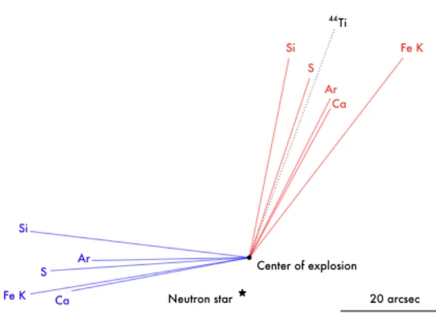
7.7 Centroids of the blue- and red-shifted parts of each line emission and their distance from the center of explosion of Cassiopeia A . . . 84

7.8 Angles between the directions of the red- and blue-shifted centers of emission from the center of explosion for each element. . . 84

7.9 Image of the Fe K red-shifted component overlaid with the extraction regions used for a44_Ti NuSTARstudy . . . 85

8.1 Images of the synchrotron retrieved by pGMCA on three energy bands . . . 89

8.2 Boxes used to define the linear profiles at the forward shock . . . 90

8.3 Linear profiles at the forward shock . . . 90

8.4 Boxes used to define the linear profiles at the reverse shock . . . 91

8.5 Linear profiles at the reverse shock . . . 91

8.6 Boxes used to define unidentified linear profiles . . . 92

8.7 Unidentified linear profiles. . . 92

9.1 The Perseus galaxy cluster in X-rays, as seen by Chandra . . . 95

9.2 H↵ emission of Perseus. . . 96

9.3 Images of the three components retrieved by pGMCA in Perseus . . . 97

9.4 Spectrum of the filament component retrieved by pGMCA . . . 97

CHAPTER

1

GENERAL INTRODUCTION

FIGURE 1.1: Tycho Brahe observing a “ stella

nova ”, the supernova SN1572. Engraving ap-pearing in the Historical book “ Astronomie Pop-ulaire ” by Camille Flammarion (Paris, 1884).

His eyes plunged into the deep black sky, Tycho Brahe noticed a luminous spot he had never seen before. “ Gosh ! he marveled, what in heaven is this wizardry ? ” He squinted, reducing his eyes to a thin slit and trying to focus. Neither the heady scent of the lilies nor the solemn call of the midnight owls could distract him from his observation, for he was absorbed in a tempest of contradictory thoughts storming his brains. “ Could this ever be ?... ”, he wondered out loud, and without even concluding his thought, he jumped to his feet and ran through his laboratory, desperately searching for some parchments and ink. “ I must take notes, he mumbled, lest this all ends up as in a dream ! ” He found what he needed and limped hurriedly back to his balcony. “ Thank God, it is still here ! ” he cried out, and immediately started to scribble. “ This is going right down in History ! ” he exclaimed happily, fully aware of his newly assigned task and willing to devote himself completely to its fulfillment. “ God has made me His humble servant, and I shall be worthy ! ” For hours and hours he took measures and scribbled unremittingly, without noticing the night fading out and the sky lightening leisurely. When he could no longer see what he thought as a new star, it was already day.

1.1

Supernovae

FIGURE 1.2: Star map of the constellation

Cassiopeia showing the position of SN1572 (labelled I). Taken from Tycho Brahe’s De

nova stella.

Supernovae have played a major role in the history of astronomy and astrophysics. Tycho Brahe in 1572 and Johannes Kepler in 1604 were the first occidental astronomers of our era to notice what they interpreted as a new star appearing for a limited dura-tion in the sky, calling the phenomenon “ stella nova ” (see Fig-ure1.1and1.2).

We can find mentions of similar events in other cultures : Arabic, Korean or Chinese manuscript mention phenomena we can now interpret as supernovae. The ancient records show a real concern for precision in their description and their centuries long registers, informing us on the importance that was given to the observation

Chapter 1 - General introduction 2

of the sky, mainly for religious or divinatory reasons. In old Chinese manuscripts, no less than a few dozens of supernovae are related, the oldest dating back to 1500 B.C.

However, the events observed by Tycho Brahe and Johannes Kepler were those that played the most im-portant role among all historically known supernovae. They happened in a time of change in the mentality of erudites, who were keen to accord a closer attention to the physical understanding of natural events than to their metaphysical meaning. Opposing other observers arguing that the “ stella nova ” he observed was something happening in the Earth’s atmosphere, Tycho Brahe measured the parallax of the object, and noted that it did not move, showing it had to lie far away. Galileo later used this as an argument against the Aristotelian view of the immutable heavens residing beyond the moon. In that way, the “ stella novae ” contributed to the philosophical change that gave birth to our modern occidental science, supporting the idea that the sky was not a flawless, unmoving and divine entity but a part of nature that could be studied and described as such.

1.1.1

Classification

As it turned out, the new stars observed by Tycho Brahe and Johannes Kepler were actually exploding dying stars. The phenomenon, now called “ supernova ”, is a transient astronomical event releasing an extraordinary amount of energy of about 1053_{erg, most of it being released in the form of neutrinos ; about}

1% in kinetic energy transfers to the ejecta and about 0.01% is converted into electro-magnetic radiation. It is visible in the optical domain before fading over several weeks or months. In 1941, Rudolph Minkovski introduced a classification that is still in use. Initially, it was based only on the spectrum, now it uses the light curves and the absorption lines of different chemical elements appearing in their spectra. It does not take into account the nature of their progenitor or their mechanisms of explosion, that were not known at that time.

FIGURE1.3: Schematic light curves for supernovae of

Types Ia, Ib, II-L, II-P, and SN 1987A. The curve for supernovae Ib includes SNe Ic as well, and represents an average. For supernovae II-L, supernovae 1979C and 1980K are used, but these might be unusually lu-minous. FromWheeler & Harkness(1990).

This classification separates Type I supernovae showing no hydrogen lines in their spectra from the Type II, that show hydrogen. Type Ia supernovae present a singly ion-ized silicon line at 615 nm, while Type Ib and c show no silicon absorption feature, or a weak one. The separation between these two subtypes relies upon the presence or not of helium in the spectra : Type Ib shows a non-ionized helium line at 587.6 nm while Type Ic supernovae show no helium line, or a weak one.

Type II supernovae can also be separated into subtypes based on the morphology of their lightcurves. Some of them show hydrogen in the beginning, but over a period of weeks or months are dominated by helium lines, re-sembling Type Ib supernovae : they are classified as Type IIb. Most of the Type II supernovae have broad emission lines ; those that have narrow features in their spectra are classified as Type IIn. Among the other ones, the su-pernovae whose lightcurve reaches a plateau are labelled Type II-P while the ones that do not show a distinct plateau are called Type II-L. See Figure1.3for a presentation of the typical lightcurves of each supernova types.

Chapter 1 - General introduction 3

Some supernovae do not fit correctly in any of these categories. Some additional supernovae types have been defined to described them, but generally, they are simply labelled as “ peculiar ”.

This supernovae classification has been criticized and mainly holds for historical reasons. It does not take into account the nature of the progenitor or the explosion mechanisms at stake, and the detection of an increasing number of peculiar supernovae show that the current types are not relevant to describe every supernovae. Also, imposing a discrete classification on an imperfectly understood phenomenon can be misguiding and distort following interpretations. For these reasons, even if detection programmes still use this classification, recent papers mainly classify supernovae in two categories reflecting better the underlying physics of the explosion mechanisms : core-collapse supernovae and thermonuclear supernovae.

1.1.2

Thermonuclear supernovae

FIGURE1.4: Two simulations of a Deflagration to

Det-onation Transition in a Type Ia, presenting two ig-nition setups. On the left, the setups include three ignition kernels (N3). On the right, they include a hundred ignition kernels (N100). The top row shows the rising plumes of the deflagration level set (white) during the Rayleigh-Taylor-unstable stage of the de-flagration phase embedded in a volume rendering of the density (in g.cm−3_{). The middle row shows the}

density and deflagration level-set structure at the time the first DDT occurs. The bottom row shows the sub-sequent spreading of the detonation level set (blue) from the DDT initiation sites. The small number of ig-nition kernels necessarily leads to a highly asymmet-ric seed configuration of the RT-unstable deflagration plumes, which can be noticed in the N3 case. From

Seitenzahl et al.(2013).

Type Ia supernovae represent about 30% of all super-novae in our Galaxy (seePtuskin et al.,2010), and have a progenitor type and mechanisms of explosion different from the Type Ib, Type Ic and Type II supernovae. They occur in binary systems, where a white dwarf accretes matter until it can no longer support its own weight. This accretion of matter can be the result of two scenarii. In the single degenerate scenario, the white dwarf forms a binary system with a more massive star. Gas from the companion star is stripped to form an accretion disc around the white dwarf.

In the double degenerate scenario, the binary system is composed of two white dwarves. Their orbit decaying, they merge ; if the mass of the resulting star is sufficient, it will explode. We still do not have a precise idea of the relative quantity of single and double degenerate sce-narii.

The temperature in the core increases with the mass, which results in a convection period. At some point, an ignition occurs, whose mechanism is still unknown. Sim-ulations seem to indicate that there needs to be some asymmetries in the distribution to spark the ignition. The burning is then propagating through a thin com-bustion wave. Current Deflagration-to-Detonation Tran-sition models (DDT) assume the combustion wave prop-agates as a deflagration due to micro-physical transport processes, releasing energy by reactions in the burning zone. Conduction and diffusion lead to heating of the fuel ahead of this zone so that it also reaches conditions for burning (see R¨opke, 2017). The propagation then evolves into a detonation, where the shock wave pro-gresses by compressing and heating fuel material so that

Chapter 1 - General introduction 4

it starts to burn, releasing, in turn, the energy to further support the shock wave. The temperature increase enhances the reaction rates, releasing energy that also raises the reaction rate. Unlike deflagrations, the propagation is not determined by microphysical transport processes but by hydrodynamical effects, leading to a faster, supersonic propagation (seeR¨opke,2017).

However, the reason for this spontaneous transition of the burning mode from a subsonic deflagration to a supersonic detonation in an unconfined medium is still unknown. Zel’dovich et al.(1970) proposes a model requiring a preconditioning of the fuel material with hot spots that would endure autoignition. This configuration may lead to a runaway of the reactions with a phase velocity sufficient to evolve into a detonation wave. It has been speculated that sufficiently strong turbulences in the deflagration burning could create these hot spots, but it is difficult to identify such regions in simulations. Therefore, several simulations artificially prescribe these spots or trigger the transition to detonation once the deflagration flame reaches a certain density threshold (see Figure 1.4). Simulations presented in Poludnenko et al.

(2011) propose another transition model, in which hot spots are not necessary. An overpressure rises in the thin combustion wave, increasing the pressure which compresses and heats up the combustion wave. This increases the propagation speed, leading to further fuel compression and giving birth to a strong shock within the thin combustion wave, creating in turn the conditions in which a detonation can arise.

Within a few seconds after the beginning of the detonation, carbon and oxygen fuse to produce heavier elements and the star violently explodes, releasing an energy of 1051 _{erg and producing a shock wave in}

which matter from the progenitor is ejected at about 30, 000 km.s 1_.

1.1.3

Core-collapse supernovae

Type Ib and c and Type II supernovae are the results of massive stars of more than 8 M undergoing core collapse when the pressure induced by nuclear fusion can no longer counter the effects of gravity. The core collapses into a neutron star (or a black hole for the heaviest progenitors) and the outer layers of the star are ejected.

It has been proven that the bounce of the forming neutron star, or proto-neutron star, was not sufficient to produce the shock wave ejecting the outer layers of the progenitor. A popular theory to explain the explo-sion mechanisms is the heating by the expelled neutrinos of the outer layers. After the matter collapses and bounces on the proto-neutron star, the shock is stalled. The neutrinos then heat up the ejecta, enough to re-vive the shock. The presence of oscillating and sloshing instabilities makes this mechanism more efficient by bringing closer to the proto-neutron star parts of the shock front, simplifying the heating. Some simulations have shown this mechanism could transfer enough energy to the outer layers to initiate the shock ; however, it may not be sufficient to explain the most energetic supernovae. Magnetohydrodynamic mechanisms, in particular in rapidly spinning stars, can also play a role by extracting energy from the highly magnetized neutron star to violently expel the outer layers of the progenitor (seeJanka, 2012, for a discussion about possible explosion mechanisms).

Observations show that the newly created neutron star is ejected with a certain velocity from the center of explosion. The kick mechanisms necessary to initiate this ejection are not perfectly understood yet, but the proposed models usually need to assess the existence of asymmetries in the original explosion. An asymmetric initiation of the explosion can indeed impart a kick to the neutron star due to linear momentum conservation (“ gravitational tug-boat mechanism ” ; see Figure1.5). An asymmetric expulsion of gas would also conduce to hydrodynamical interactions between the proto-neutron star and the ejecta, which would be coupled with an anisotropic gravitational pull of the ejecta on the proto-neutron star, inducing a kick. An

Chapter 1 - General introduction 5

anisotropic neutrino emission has also been considered as a potential neutron star kick mechanism. In any case, asymmetries seem to be a key element to understand fully the core-collapse explosion mechanisms and the observed neutron star kick.

FIGURE 1.5: Entropy-isosurfaces (left) of the SN shock (grey) and of the high-entropy bubbles (green),

ray-casting images of the density (middle), and entropy distribution in a cross-sectional plane (right) for two models of core-collapse supernova simulations at about 1.3 s and 1.4 s after core bounce. The viewing directions are normal to the plane spanned by the neutron star kick and spin vectors of each model, which also defines the plane for the entropy slices. The SN shock has an average radius of 13,000 km and 14,000 km for each model, respectively (a length of 5000 km is given by yardsticks below the left images). The kick and spin directions are indicated by the white and black arrows, respectively, in the middle figures. The neutron star locations are marked by black crosses in the right plots. The images in the middle correspond roughly to the projections of the density distribution on the observational planes. Dilute bubble regions are light-colored in white and yellow, while dense clumps appear more intense in reddish and bluish hues. The purple circular areas around the neutron star represent the dense inner region of the essentially spherically symmetric neutrino-driven wind. The wind is visible in green in the right images and is bounded by the aspherical wind-termination shock. The neutron star is clearly displaced from the geometrical center of the expanding shock in the direction of the kick vector pointing to the lower left for the model on top. The neutron star in model on the bottom has a much smaller kick velocity, and does not show any clear displacement but remains located roughly at the center of the expanding ejecta shell. FromWongwathanarat et al.(2013).

Chapter 1 - General introduction 6

Summary :

• A supernova is the explosion of a star that we call its “ progenitor ”.

• There are two main types of supernovae : the Type Ia, or thermonuclear supernovae, and the core-collapse supernovae.

• Thermonuclear supernovae are the results of white dwarves accreting from a companion star in a binary system, either by accreting gas from a stellar companion (single degenerate scenario) or by merging with another white dwarf (double degenerate scenario). Reaching a certain mass ignites a thermonuclear reaction leading to the explosion.

• Core-collapse supernovae are caused by massive stars (> 8 M ) in which the pressure induced by nuclear fusion can no longer counter the effects of gravity. The core forms a neutron star or a black hole, and the outer layers are ejected.

• For both supernovae types, some key elements are still missing to understand fully the explosion mechanisms. In both cases, the presence of instabilities and asymmetries in the explosion seems to be a key ingredient.

1.2

Supernovae remnants

FIGURE 1.6: Scheme presenting the structure of

a SNR. The compact object, present only in core-collapse supernovae, is either the neutron star or the black hole formed by the collapse of the progenitor’s core.

Whatever the supernova type, the explosion ends up expelling stellar material at velocities of about 30, 000 km.s 1_{. Ahead of these ejecta, a powerful shock wave}

forms that heats up the interstellar medium to temper-atures up to million degrees tempertemper-atures. The shock wave is progressively slowed down by the interstellar medium, but it continues its expansion for several thou-sands years. These objects are called supernovae rem-nants (SNRs).

Heated material from the ejecta or the shocked interstel-lar medium emit electro-magnetic radiations long after the end of the explosion. Through these radiations, the SNRs can be observed. A gas heated at 107_{K will have its}

thermal emission peaking in the X-ray band, making the X-rays an appropriate domain to observe SNR. They are also visible in radio and gamma-rays through the radia-tion of the particles they accelerate.

Most SNRs can be seen in X-rays or gamma-rays, but some of them can also be detected in the optical domain.

Chapter 1 - General introduction 7

1.2.1

Supernovae remnants stages

The evolution of a SNR over time can be divided into three phases. During the first one, the SNR is in free expansion. The front of the expansion is formed from the shock wave heating up the interstellar medium to approximately 107_{K and expanding in the forward direction. The contact of the interstellar material causes}

a second shock to form, directed in the reverse direction (see Figure 1.6). This reverse shock goes back through the ejecta, heating it up. The forward shock pushes the interstellar medium into an expansive shell whose expansion velocity is constant. This phase can last for a few hundred years, until the mass of the interstellar material swept up by the shock exceeds the phase of the ejected material.

FIGURE 1.7: Radius (left) and velocity (right) during the

evo-lution of a SNR in a wind-blown cavity, surrounded by a dense, swept-up shell. FromDwarkadas(2007).

The second one is the Sedov phase, during which the ejecta begins to decelerate, its veloc-ity evolving in proportion to t 3/2_{, t being the}

age of the SNR (see Figure 1.7). During this phase, Rayleigh-Taylor instabilities arise once the mass of the swept up interstellar medium approaches that of the ejected material, mix-ing the ejecta with the shocked gas from the interstellar medium. This phase lasts for a pe-riod spanning from a few thousands years to about 20, 000 years.

The last phase, or radiative phase, begins after the shell has cooled down to a temperature of less than 106

K. Electrons start recombining with the heavier atoms, making the shell radiate energy more efficiently. This results in cooling down the shell faster, making it thiner and denser. The more the shell cools down, the more atoms can recombine ; hence, the shell slims down and the SNR radiates most of its energy as optical light. The velocity then decreases in proportion to t 3_{and the expansion of the shell stops. This period lasts}

for a few hundred of thousands years. After millions of years, the SNR will be completely diluted into the interstellar medium thanks to the Rayleigh-Taylor instabilities forcing the mixing of the SNR material.

1.2.2

Acceleration in SNRs and cosmic rays

With 1051_{erg released in kinetic energy during the explosion, SNRs are ideal sites to accelerate particles and}

are thought to be the main source of galactic cosmic rays. The ion acceleration can be very efficient to trans-fer kinetic energy, especially in shocks parallel or quasi-parallel to the background magnetic field : about 10% to 20% of the bulk flow energy is channeled in energetic particles (Caprioli & Spitkovsky,2014a). These particles induce a turbulent amplification of the magnetic field around the shock that will in turn contribute to accelerate particles from the interstellar medium. This magnetic field possesses inhomogeneities that are enhanced by the particles themselves. Thus, a moving particle entering the shock front will be accelerated through the diffusive shock acceleration mechanism : the particle arriving upstream and going downstream through the shock will encounter a moving change in the magnetic field that will reflect it again through the shock. The process can repeat itself several times, the particle gaining energy such that ∆E

E = ∆Vc at each

crossing until it finally escapes. See Figure1.8for a presentation of a simulation of this phenomenon. Through this process, particles from the interstellar medium can be accelerated by SNRs. Recent obser-vations and simulations have proven that at least a part of the cosmic rays we can observe are produced this way. However, there are still questions about the acceleration and liberation mechanisms and about the most energetic galactic cosmic rays (more than 1015_{eV) that the current simulations fail to reproduce.}

Chapter 1 - General introduction 8

FIGURE1.8: Relevant physical quantities for a parallel shock. From top to bottom : ion density, modulus and

three components of the magnetic field, in units of their respective initial values. We can see the turbulent magnetic field generated by the accelerated ions.Caprioli & Spitkovsky(2014b).

Nevertheless, SNRs appear to be essential in our understanding of cosmic rays, and a better knowledge of the acceleration mechanisms would make us know if there needs to be any other sources to account for the existence of the most energetic cosmic rays.

1.2.3

Asymmetries in supernovae remnants

Expelled at a spectacular speed from the center of explosion, the shock rapidly expands to form a large astronomical object of a typical size of several parsecs after a few centuries. This large size allows us to obtain precise images of the remnants even at kpc distances and thus study their morphology.

In particular, the study of asymmetries in SNRs, either on their global shape materialized by the front shock or on the repartition of each individual elements, may bring some information about the mechanisms of ex-plosion at stakes in the original supernova. Although the asymmetries of the surrounding medium crossed by the forward shock also have a clear impact that is difficult to decorrelate from hypothetical asymmetries

Chapter 1 - General introduction 9

in the explosion, some observations and simulations concur to assert their existence. Jet-like structures that have been observed in several core-collapse SNRs are for example thought to be the direct consequence of their explosion mechanism. Orlando et al.(2016) has explored the evolution of the asymmetries in Cas-siopeia A thanks to simulations beginning from the immediate aftermath of the supernova and presenting the 3D interactions of the remnant with the interstellar medium. Similar simulations presenting the evolution of a Type Ia SNR over a period spanning from one year after the explosion to several centuries afterwards have been made byFerrand et al.(2019), showing that asymmetries present in the original supernova can still be observed after centuries. These results show how the observation of asymmetries in SNRs can help constraining and understanding the explosion mechanisms in supernovae.

Summary :

• In supernovae remnants (SNRs), the front shock still expands after centuries, heating up the interstel-lar medium.

• Another shock wave is produced, directed towards the center of the explosion, heating up the ejecta, the matter expelled from the progenitor.

• A strong magnetic field develops around the shock. It can trap particles, while the shock accelerates them until they are released. At least a part of the galactic cosmic rays we can observe are produced by this phenomenon.

• Some asymmetries in the explosion in supernovae can still be observed after centuries in SNRs. An extensive study of asymmetries in SNRs could help understanding the mechanisms of explosion in supernovae.

Chapter 1 - General introduction 10

FIGURE1.9: Slices of the mass density at t = 1 yr (top), 100 yr (middle), and 500 yr (bottom) of the evolution

of two simulations of SNRs. The left side shows the case of spherically symmetric ejecta (effectively 1D initial conditions), while the right side shows the case of asymmetric ejecta (fully 3D initial conditions). Note that the color scale is logarithmic and that its upper value is adjusted over time so that all frames have similar contrast (the density in the inner ejecta decreases by several orders of magnitude over this period). From

Chapter 1 - General introduction 11

1.3

Supernovae remnants in X-rays

SNRs can still be detected long after the end of the explosion itself, because the hot gas and the accelerated particles still radiate in a large range of wavelengths (see Figure1.10). In this thesis, we will focus on the observation of SNRs in X-rays ; hence, we will describe the different types of emission in this domain and the current instruments allowing us to observe them.

1.3.1

Continuum emissions

There are five mechanisms that can produce continuum X-ray emission in SNRs, two non-thermal (the synchrotron emission and the comptonization), and three thermal (the bremsstrahllung, the free-bound emission and the two-photon emission). These radiations are continuous, because they are caused by a variation of velocity of electrons, and the population of electrons can reach a continuous range of energies.

FIGURE 1.10: Cassiopeia A in X-rays as seen by the

Chandra X-Ray Observatory. The synchrotron emission is in blue, other colors correspond to thermal emis-sions.

The first mechanism, the synchrotron radiation, is linked to the magnetic field and to the particles it accelerates. It is emitted when an electron interacts with the magnetic field that will cause the electron to change its direction by exerting a force perpendicular to its original direction. The electron will then be accelerated, and radiate elec-tromagnetic energy. This radiation can range over the en-tire electromagnetic spectrum, including X-rays in young SNRs.

The comptonization happens when a photon collides with an electron. If the photon gives energy to the elec-tron, accelerating it, the effect is named “ Compton scat-tering ”. If the electron gives energy to the photon, the effect is named “ Inverse Compton scattering ”.

The thermal bremsstrahlung occurs when an electron passes close to a ion in a hot gas, the strong electric forces causing its deceleration and a change in its

trajec-tory. The electron will lose kinetic energy, which will be converted into radiation. In a gas with a temperature of some millions of degrees Kelvin as in SNRs, the radiation will peak in the X-ray band.

The free-bound emission arises when an electron is captured into one of the atomic shells. Free-bound emis-sion mainly looks like a bremsstrahlung because it is not quantised and follows a Maxwell-Boltzmann dis-tribution. In photo-ionized or overionized plasmas, it can possess line-resembling features called radiative-recombination continua.

Two-photon emission results from electrons in meta-stable states. If they are not de-excited by a collision, which is likely in rarified plasmas of SNRs, it can de-excite by emitting two photons.

In SNRs, the gas heated by the explosion, either from the ejecta or the interstellar medium, reaches temper-atures at which most of its thermal emissions in X-rays will be caused by thermal Bremsstrahlung and line emissions. However, the parameters characterizing the different thermal emissions are not easy to retrieve as the plasmas formed by the hot emitting gas are often out of ionization equilibrium, because with the

Chapter 1 - General introduction 12

low densities involved, not enough time has passed for enough collisions to happen in order to reach an equilibrium.

The presence of highly energetic electrons and the strong magnetic field can also be important sources of X-rays in SNRs through the synchrotron radiation. As it is located at the forward shock, these emissions give useful information about the location of the forward shock and insights about the acceleration mechanism taking place.

1.3.2

Line emissions

Another type of features that are emitted in X-rays in SNRs is the line emission associated with the different elements of the ejecta or of the heated interstellar medium. These emissions result from collisional excitation of ions, often through an electron-ion collision, and radiate at a precise energy characteristic of the emitting element and of its ionization state.

FIGURE1.11: Thermal X-ray theoretical emissions between

0.5 and 10 keV (panel a) and around the Fe K line complex (panel b) of an optically thin transient plasma with solar abundances and electron temperature T e = 3 ∗ 107

K, for three values of the ionization parameter. For net = 10

13

cm−3_{.s, the plasma has reached the ionization equilibrium.}

FromTatischeff, V.(2003).

In plasmas that have not reach their ionization equi-librium, there can be inner shell ionization. In this process an electron from an inner shell can be re-moved while higher atomic levels are still filled. The ion can then de-excite without radiation by fill-ing the hole or adjust radiatively, which is called fluorescence. The likelihood for a radiative tran-sition, the fluorescence yield, is higher for atoms with larger nuclear charge. Because of its high fluo-rescence yield and high abundance, the Fe K-shell emission can be observed at all ionization states of iron if the electron temperature is high enough. For that reason, the iron line emission is an im-portant diagnostic tool to evaluate the state of an SNR plasma through its average electron tempera-ture and ionization age net. By combining

informa-tion from the continuum and line emissions in X-rays we can measure properties of the plasma such as the electron temperature, the ionization states and the abundances of the different elements, from oxygen to iron (see Figure1.11).

In general, being able to retrieve maps correspond-ing to every line emissions gives fruitful information about the spatial distribution of each element. This

way, we can link their behaviors to their individual properties for a better understanding of the evolution of the original progenitor’s layers after the explosion. We can also have an insight on the asymmetries in the ejecta for each individual element, which could help to understand the explosion mechanisms.

Chapter 1 - General introduction 13

1.3.3

Spectro-imaging instruments in X-rays

FIGURE1.12: Artist’s impression of the Chandra X-Ray

Observatory.

X-rays being absorbed by Earth’s atmosphere, the tele-scopes to detect them have to be carried by satellites orbiting above it. Unlike optical telescopes, X-ray tele-scopes possess almost cylindrical mirrors presenting a low grazing angle in order to reflect photons that would otherwise pass through them. The X-ray detectors cap-ture photons individually, so that for each one four mea-sures are taken : its spatial coordinates x and y, its en-ergy E and the time of detection t. Hence, we call these instruments spectro-imaging instruments, and the data they capture takes the form of an hypercube (x, y, E, t). As SNR are not evolving fast enough for the time of de-tection to be an important factor, we will consider the data to be of the form of a cube (x, y, E).

FIGURE1.13: Artist’s impression of the XMM-Newton

spacecraft.

The two main spectro-imaging instruments currently in activity are onboard Chandra, launched by NASA in 1999 and XMM-Newton launched by ESA the same year (see Figures 1.12 and 1.13). Chandra has the best angular resolution : 0.5 arcseconds, against approximately 6 arc-seconds for XMM-Newton, resulting in sharper images. However, XMM-Newton has a larger field of view, and its collecting area is substansially bigger than that of

Chan-dra(2, 000 cm2_{against 400 cm}2_{at 1 keV). They both have}

a similar spectral resolution (see an example of Chandra spectrum in Figure1.14, right).

The images and spectra obtained by these instruments on large astronomical objects like the SNRs are astounding, but their high quality data is not fully exploited by the

data analysis methods currently in use in this field : most of the information is often lost by considering only the spectral dimension, even if the spatial and spectral dimensions are intrinsically entangled. With the development of the future generation of X-ray space telescopes, among which Athena is the most advanced, the need of developing new tools appears even more urging. The spatial resolution of Athena will be better than that of XMM-Newton, while its spectral resolution of 2.5 eV will be outstandingly better than that of its predecessors thanks to the micro-calorimeter technology allowing to measure with great precision the energy deposited by each X-ray photon (Barret et al., 2020). The arrival of such a new spectro-imaging instrument could bring an amazing quantity of new data to evaluate and improve our current knowledge on high energy astrophysics. However, we will need to develop better data analysis methods than those currently in use to fully exploit the potential of the new generation of spectro-imaging instruments.

1.3.4

Traditional data analysis methods in X-rays

Current data analysis methods in use in supernova remnant studies rarely involve a separation on the en-tangled components. They mostly consist in defining areas of interest in the data set flattened as an image, and extracting the spectra from these areas (see Figure 1.14for an illustration). They are then processed

Chapter 1 - General introduction 14

FIGURE1.14: On the left, the same image as in Figure1.10. On the right, Cassiopeia A’s spectrum in X-rays as

seen by the Chandra X-Ray Observatory1_{. The area surrounded by a red box figures an area of extraction for}

the spectrum, but does not correspond to the actual spectrum presented here. It has been added for illustrative purposes only.

through a software such as Xspec, where physical models chosen by the user are fitted in order to retrieve physical parameters such as the temperature, the abundance, the metallicity... As the user has to define the fitted models, a certain amount of prior physical information is needed. The different physical components also remain entangled as this kind of methods only produce a set of parameters, possibly from different components, without separating these components. When applied on a sufficient number of areas map-ping the total remnant, maps of the parameters can be produced, but doing them is highly time consuming and the resulting images are poorly detailed. The total information contained in the (x, y, E) original data cube is not used, as the whole information is retrieved only on the spectra, and the areas of extraction are considered individually, thus neglecting the high correlation between them.

FIGURE1.15: The Mg emission structure in

Cas-siopeia as retrieved with traditional data anal-ysis methods. On top, extract from Figure 9 of

Lopez et al.(2011). On the bottom, extract from Figure 2 ofHolland-Ashford et al.(2020).

We see inLopez et al.(2011) an example of component sepa-ration. In order to conduct this study, images of the different line emission structures in chosen SNRs was needed. They were obtained by integrating the data around the peak of each line emission, thus producing images of the emission struc-tures still strongly polluted by other components such as the synchrotron continuum (see Figure 1.15). Other traditional methods involving component separation usually involve the use of Xspec on chosen areas to separate components in the spectra, and produce maps of the areas showing where each component is mainly present. As for the parameters map ob-tained in a similar way, the results are poorly detailed and do not exploit fully the information from the original data. The resulting images are also difficult to use, as the pixel values do not represent number of counts (see for example Holland-Ashford et al.,2020, see Figure1.15)

The aim of this thesis is to explore a new data analysis method for component separation using both the spectral and spatial dimensions in order to exploit as much as possible the informa-tion contained in the X-ray data. In a first part, we will present the mathematical objects needed to develop our method. We will then explain the method, test it and propose a way to re-trieve error bars attached to the results. In a second part, we

Chapter 1 - General introduction 15

will show some applications of our method on real data, proving its usefulness to actually obtain results that could not have been obtained otherwise. Our first application will be on asymmetries in the SNR Cassiopeia A, in an attempt to map the repartition of the different line emissions and quantify their relative asymme-tries, thus providing new information on a key topic in SNRs studies. Our second application will focus on the synchrotron rims that can be seen in X-rays in some SNRs. We will investigate the dependency of their widths with energy. The last application will be an attempt to test our method on another kind of extended sources in X-rays : the Perseus galaxy cluster. More specifically, we will search for an X-ray counterpart to the filaments visible in the H↵ emission.

Summary :

• SNRs can be visible in X-rays. The matter heated up by the front or the forward shocks is hot enough for the thermal emission to peak in X-rays. Some non-thermal radiation processes also emit in X-rays. • Among the thermal emissions in X-rays, the thermal bremsstrahlung and the line emissions are the most important. The line emissions characterize the chemical element by which they were emitted, thus allowing to map the presence of a certain element in a SNR by considering the sources of its line emission.

• Among the non-thermal emissions in X-rays, the synchrotron emission is the most important. It is caused by the accelerated particles radiating in an amplified magnetic field at the shock, allowing us to study the properties of accelerated electrons and the acceleration mechanism.

• X-ray telescopes such as Chandra and XMM-Newton contain spectro-imaging instruments producing data cubes composed of two spatial and a spectral dimension.

• Current data analysis methods in use in high energy astrophysics do not fully exploit the wealth of the existing and future spectro-imaging instruments. We intend in this thesis to provide a new data analysis method using both the spectral and spatial dimensions in order to exploit as much as possible the information contained in the X-ray data cubes.

Part I

Methodology

CHAPTER

2

WAVELETS

Wavelets constitute a wide and rich mathematical fields particularly flourishing nowadays, with many ap-plications on a large variety of subjects. A proper presentation of the formalism necessary to define and use wavelets in 2D on images going far beyond the scope of this thesis, we will only introduce them through their original one dimensional definition. The passage to two dimensions will not be presented in general, but only applied on the specific algorithm we will use later, the “ `a trous ” algorithm.

2.1

Wavelets in one dimension

In this thesis, we will only use a two-dimensional kind of wavelets. However, it is far easier to understand the principle and the properties of the wavelet transforms by studying their original definition in one di-mension. In this Section, we will introduce the continuous wavelet transforms in one dimension and their discretization to adapt them for actual computation.

2.1.1

Continuous wavelet transforms in one dimension

A wavelet is a square-integrable function of zero mean. Basically, a wavelet transform consists in a mother wavelet and the child wavelets a,bobtained through scaling and translation of :

a,b(t) =

1

p_a ✓ t _ab ◆

(2.1)

where a is a positive real defining the scale and b is a real number defining the shift. See Figure2.1for a classical example of mother wavelet.

It is possible to project a function f 2 L2_{(R) onto the subspace of scale a :}

fa(t) =

Z

R

W Tψ{f }(a, b) · a,b(t)db (2.2)

where the wavelet coefficients W Tψ{f }(a, b) are defined as :

W Tψ{f }(a, b) = hf, a,bi =

Z

R

f (t) a,b(t)dt (2.3)

It can be rewritten as a convolution product, by defining :

Chapter 2 - Wavelets 20 a(t) = 1 p a ✓ _t a ◆ (2.4) Leading to : W Tψ{f }(a, b) = Z R f (t) a(t b)dt = f ? a(u) (2.5)

FIGURE 2.1: A classical example of a mother

wavelet, the “ Mexican hat ”.

Wavelet transforms can measure the time evolution of fre-quency transients. The decay of W Tψ{f }(a, b) when the scale

a goes to zero characterizes the regularity of f in the neigh-borhood of b (see Figure2.2). In the regions where f is regu-lar, the wavelet coefficients rapidly decay to zero. Hence, the wavelet transforms give information about the details of f at different scales : each scale is sensitive to the variations in frequency of this certain scale. This specificity will prove par-ticularly useful when generalized to two-dimensional images. Wavelet transforms preserve the information and can be in-verted : f = W T 1 ψ {W Tψ{f }}. t t sca le t _t sca le

FIGURE 2.2: Two examples of functions and their wavelets transform for scales 1 to 10 obtained with the

Mexican hat wavelet. The scale increases from top to bottom. Color bars were not added for clarity : the dominant grey corresponds to 0, lighter shades are positive and darker negative. We can see the wavelet coefficients are non-zero only where the original function’s variating, i.e. where the, and only the concerned scales are sensitive to the variations. In the first example, the variation being infinitely small, it is apparent at every scale : even by zooming infinitely around the point of discontinuity of the derivative, this variation can still be seen. However, in the second example, the variations are smoother : if we zoom enough, the slope will appear to be constant. For that reason, the wavelet coefficients of the second example are only sensitive to the variations of certain scales : fast variations are already visible with coefficients of small scale, while slower variations only appear for largest scales.

2.1.2

Discrete wavelet transforms

Actual computations are made on discrete signals, so it appears necessary to discretize the wavelet trans-forms.

Let f (t) be a continuous time signal uniformly sampled in N intervals over [0, 1]. We note f [n] = f (n) the signal of size 1/N on the n-th interval. By choosing a wavelet whose support is included in [ K/2, K/2] we can define, for 2  aj_{ NK} 1_{a discrete wavelet scaled by a}j _:

Chapter 2 - Wavelets 21 j[n] = 1 p aj ✓ n aj ◆ (2.6)

The discrete wavelet we obtain has Kaj _{non-zero values on [ N/2, N/2]. The scale a}j _{must be larger than}

2 to avoid the sampling interval being larger than the wavelet support. The discrete wavelet coefficients can thus be defined :

wψ{f }(n, aj) = N 1 X m=0 f [m] j[m n] = f ? j[n] (2.7) where _j[n] = j[ n].

Summary :

• The wavelet transforms of a one-dimensional function give information about the regularity of this function at different scales.

• It is possible to discretize the wavelet transforms by considering only a discrete set of scales.

2.2

A particular case of two-dimensional wavelets

In this Section we will present the particular case of the starlet transform, that we will use later in the thesis. The passage from one to two dimensions in this particular case is made through the “ `a trous ” algorithm that we will first describe.

2.2.1

The “ `

a trous ” algorithm

The “ `a trous ” algorithm is based on a dyadic discrete transform, which means that we choose a equal to 2. The main idea of the algorithm is to build an undecimated wavelet transform : it keeps the set of coefficients wjof the same size as the original signal for each scale, making it redundant (seeStarck et al.,1998).

The “ `a trous ” algorithm builds a sequence of approximations of an N -sized signal f0at increasingly larger

scales {f1, · · · , fJ}. Each approximation is obtained from the previous one through a convolution with a

mother wavelet filter ¯h(j)_{at scale j + 1 :}

fj+1[n] = (h(j)?fj)[n] (2.8)

the first approximation f1being a direct application of the filter ¯h(0)on the signal f0.

According to the “ `a trous ” algorithm, consecutive filters h(j) _{are obtained by adding zeroes between the}

Chapter 2 - Wavelets 22

The set of wavelet coefficients wj+1at scale j + 1 are then defined as the difference between consecutive

large-scale approximations :

wj+1[n] = fj[n] fj+1[n] (2.9)

Note that the details at scale j + 1 are obtained by subtracting the smoothed approximation fj+1from the

approximation fj. This way, only the structures that disappeared in the smoothing at scale j + 1 are kept in

wj+1.

This eventually yields a decomposition of the signal f0into W = {w1, ..., wJ, fJ}. The last set of coefficients

fJcontains all the information that was left over by the precedent scales coefficients. It is named the “ coarse

scale ”.

The reconstruction of the initial signal f0is then obtained by a simple coaddition of all wavelet scales and

the final smooth subband :

f0[n] = fJ[n] + J

X

j=1

wj[n] (2.10)

This algorithm can easily be generalized to two-dimensional images, as we will see with the starlet trans-form.

2.2.2

The starlet transform

The starlet transform is a special case of bi-dimensional wavelets, which has been specifically designed to efficiently represent isotropic structures in images. Therefore, this particular case of wavelets has been proved to be well-adapted to analyze astrophysical images.

The starlet transform uses a two-dimensional version of the “ `a trous ” algorithm. Here, we note c0 the

original image of size N ⇤ N. The approximations at increasingly larger scales are noted {c1, · · · , cJ} and

obtained thus :

cj+1[k, l] = (h(j)?cj)[k, l], (2.11)

where the filter h(0)_{is defined as :}

h(0)= 1 256 0 B B B B B B @ 1 4 6 4 1 4 16 24 16 4 6 24 36 24 6 4 16 24 16 4 1 4 6 4 1 1 C C C C C C A (2.12)

and the consecutive filters h(j)_{are obtained by adding zeroes between the nonzero filter elements, just as in}

the precedent Section (seeStarck et al.,2015).

The wavelet coefficients at scale j + 1 are then defined as the difference between consecutive large-scale approximations :

Chapter 2 - Wavelets 23

This eventually yields a decomposition of the image c0into W = {w1, ..., wJ, cJ}, where cJ is the “ coarse

scale ”.

The reconstruction of the initial image c0is once again obtained by a simple coaddition of all wavelet scales

and the final smooth subband :

c0[k, l] = cJ[k, l] + J

X

j=1

wj[k, l] (2.14)

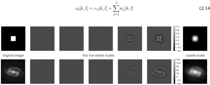
original image first five starlet scales coarse scale

FIGURE2.3: An image of a square and an astrophysical image and their starlet transforms in six scales. The

colorbar is the same for the first five starlet scales. It highlights the fact that most wavelet coefficients are zero.

Summary :

• The starlet transform has been designed to efficiently represent isotropic structures in images.

• It transforms an image into a set of images of the same size, each representing details of a certain scale. The last image is named the “ coarse scale ” and contains all the information that was left over in the other scales.

2.3

Sparsity

One of the most interesting properties of two-dimensional wavelet transforms is their sparsity : most of the information is contained in a few coefficients (seeMallat,2008).

Figure2.3shows that most of the coefficients in the three first scales of the four scales starlet transform of a square are zeros, for these scales only focus on the details of the image, here the edges. Hence, a few coefficients are sufficient to contain most of the useful information of the image, while the coarse scale (the last scale) contains what is left.

Thus, the scales before the coarse one contain mainly information about the different features in the image. The last one, from which details such as edges have been removed, consists in a blurred version of the orig-inal image and is useful to reconstruct it. For that reason, the sparsity of wavelets transforms is an essential