HAL Id: tel-00431464
https://tel.archives-ouvertes.fr/tel-00431464
Submitted on 12 Nov 2009
HAL is a multi-disciplinary open access
archive for the deposit and dissemination of sci-entific research documents, whether they are pub-lished or not. The documents may come from teaching and research institutions in France or abroad, or from public or private research centers.
L’archive ouverte pluridisciplinaire HAL, est destinée au dépôt et à la diffusion de documents scientifiques de niveau recherche, publiés ou non, émanant des établissements d’enseignement et de recherche français ou étrangers, des laboratoires publics ou privés.
implementation and analysis
Linqiao Zhang
To cite this version:
Linqiao Zhang. On the three-dimensional visibility skeleton: implementation and analysis. Computer Science [cs]. Université McGill, 2009. English. �tel-00431464�
Linqiao Zhang School of Computer Science McGill University, Montreal
September 2009
A Thesis submitted to the Faculty of Graduate Studies and Research
in partial fulfillment of the requirements for the degree of Ph.D.in Computer Science
c
Title Page . . . i
Table of Contents . . . iii
Abstract . . . vii
Résumé . . . ix
Declaration . . . xi
Acknowledgments . . . xiii
List of Figures . . . xv
List of Tables . . . xxi
1 Introduction 1 2 Background and Related Work 11 2.1 The Visibility Complex . . . 11
2.1.1 The 2D Visibility Complex . . . 12
2.1.2 The 3D Visibility Complex . . . 20
2.2 The Visibility Skeleton . . . 25
2.2.1 The 2D Visibility Skeleton . . . 26
2.2.2 The 3D Visibility Skeleton . . . 28
2.2.3 The Size Complexity of the Visibility Skeleton . . . 38
2.3 Overview of the Sweep Algorithm . . . 40
3 Experimental Study of the Size of the 2D Visibility Complex 45 3.1 Models . . . 46
3.2 Experiments . . . 48
3.2.1 Software . . . 48
3.2.2 Setting . . . 48
3.2.3 Experimental Results and Interpretation . . . 50
3.3 Summary and Bibliographic Notes . . . 59
4 An Implementation of the Sweep Algorithm 61 4.1 The Input . . . 61
4.2 The Output . . . 62
4.3 Description of the Implementation . . . 63
4.3.1 Preliminaries: The CGAL Library and Number Types . . . . 66
4.3.2 The 2D Visibility Skeleton . . . 68
4.3.3 Computing Events . . . 70
4.3.4 The Event List . . . 74
4.3.5 Updating the 2D Visibility Skeleton and the Event List . . . . 75
4.3.6 Computing the Ordering of Bitangents . . . 80
4.3.7 Computing the 3D Visibility Skeleton Vertices . . . 82
4.4 Complexity of the Implementation . . . 86
4.5 Software Validation . . . 87
4.5.1 Visualization . . . 88
4.5.2 Experimental Verification . . . 92
4.6 Performance . . . 93
4.6.1 Running Time in Terms of n and k . . . 93
4.6.2 Running Time in Terms of the Number of Polygons . . . 97
4.6.3 Running Time in Terms of Number Types . . . 101
4.7 Conclusion and Bibliographic Notes . . . 103
5 The Algebraic Degree of the Predicates 105 5.1 Computing Lines through Four Lines . . . 107
5.2 Predicates . . . 114
5.2.1 Preliminaries . . . 114
5.2.2 Transversals to Four Lines . . . 115
5.2.3 Transversals to Four Segments . . . 117
5.2.4 Ordering Planes through Two Fixed Points, Each Containing a Third (Rational) Point or a Line Transversal . . . 125
5.3 Experiments . . . 129
5.4 Discussion . . . 132
5.5 Bibliographic Notes . . . 132
6 Experimental Study of the Size of the 3D Visibility Skeleton 133 6.1 The Visibility Skeleton of a Set of Polytopes . . . 135
6.2 Setting of the Experiments . . . 136
6.2.1 The Model . . . 136
6.2.2 The Experiments . . . 137
6.2.3 Number Type and Machine Characteristics . . . 139
6.3 Experimental Results and Analysis . . . 140
6.3.1 Number of Skeleton Vertices in Terms of n . . . 140
6.3.2 Number of Skeleton Vertices in Terms of n and k . . . 141
6.4 Double versus Filtered_exact . . . 146
7 Computing the 3D Visibility Skeleton 151 7.1 Preliminaries . . . 154 7.2 Computational Relations among the Visibility Skeleton Vertices . . . 155 7.3 Recovery of the Full Skeleton . . . 160 7.4 Tightness of the Succinct Skeleton . . . 174 7.5 Discussion . . . 176
8 Conclusion and Future Work 177
On the three-dimensional visibility skeleton: implementation
and analysis
Abstract
The visibility skeleton is a data structure that encodes global visibility information of a given scene in either 2D or 3D. While this data structure is in principle very useful in answering global visibility queries, its high order worst-case complexity, especially in 3D scene, appears to be prohibitive. However, previous theoretical research has indicated that the expected size of this data structure can be linear under some restricted conditions. This thesis advances the study of the size of the visibility skeleton, namely, using an experimental approach.
We first show that, both theoretically and experimentally, the expected size of the visibility skeleton in 2D is linear, and present a linear asymptote that facilitates estimation of the size of the 2D visibility skeleton.
We then study the 3D visibility skeleton defined by visual events, which is a subset of the full skeleton defined by Durand et al.. We first present an implementation to compute the vertices of that skeleton for convex disjoint polytopes in general position. This implementation makes it possible to carry on our empirical study in 3D. We consider input scenes that consist of disjoint convex polytopes that approximate randomly distributed unit spheres. We found that, in our setting, the size of the 3D visibility skeleton is quadratically related to the number of the input polytopes and linearly related to the expected silhouette size of the input polytopes. This
estimate is much lower than the worst-case complexity, but higher than the expected linear complexity that we had initially hoped for. We also provide arguments that could explain the obtained complexity. We finally prove that, using the 3D visibility skeleton defined by visual events, we can compute the remaining vertices of the full skeleton in almost linear time in the size of their output.
Squelette de visibilité en trois dimensions: implémantation et
analyse
Résumé
Le squelette de visibilité est une structure de donnée qui encode l’information de visibilité globale pour une scène donnée en 2D ou 3D. Cette structure de donnée est en principe très utile pour répondre à des requêtes de visiblité globale, mais elle est, en particulier en 3D, d’une complexité de haut degré dans le pire des cas qui semble prohibitive. Cependant, les recherches théoriques précédentes ont indiqué que l’espérance de la taille de cette structure de donnée peut être linéaire sous certaines conditions restreintes. Cette thèse approfondit l’étude de la taille du squelette de visibilité, au moyen d’une approche expérimentale.
Nous montrons d’abord qu’aussi bien théoriquement qu’empiriquement, l’espérance de la taille du squelette de visibilité en 2D est linéaire, et présentons une asymptote affine qui facilite l’estimation de la taille du squelette de visibilité en 2D.
Nous étudions ensuite le squelette de visibilité 3D défini par événement visuels, qui est un sous-ensemble du squelette complet défini par Durand et al. . Nous présen-tons tout d’abord une implantation calculant les sommets de ce squelette pour des polytopes convexes disjoints en position générale. Cette implantation nous permet de continuer notre étude empirique en 3D. Nous considérons des scènes données consis-tant en des polytopes convexes disjoints qui sont une approximation de sphères unités distribuées aléatoirement. Nous avons découvert que, dans ces conditions, la taille
du squelette de visibilité 3D a une relation quadratique en le nombre de polytopes donnés, et linéaire en l’espérance de la taille de la silhouette des polytopes donnés. Cette estimation est bien plus basse que la complexité dans le pire des cas, mais plus haute que la complexité linéaire que nous espérions initialement. Nous présentons aussi des arguments qui pourraient expliquer la complexité obtenue. Nous prouvons finalement qu’en utilisant le squelette de visibilité 3D défini par événement visuels, nous pouvons calculer les sommets restants du squelette complet en temps presque linéaire en la taille du résultat.
This thesis contains no material which has been accepted in whole, or in part, for any other degree or diploma. Chapters 3 to Chapter 7 present new contributions to knowledge. Some of the results have already appeared in conferences or journals. My contribution to the research described in each of the chapters is given in detail as follows.
• Chapter 3 is based on joint research with Hazel Everett, Sylvain Lazard and Sylvain Petitjean. I contributed significantly to the research, and conducted all the experiments except those in the Section 3.2.3 "Analysis for low densi-ties", which were conducted by Hazel Everett. I included this section here for completeness.
• Chapter 4 is my own work.
• Chapter 5 is based on joint work with Hazel Everett, Sylvain Lazard and Bill Lenhart. I contributed significantly to the research, and also I conducted the experiments.
• Chapter 6 is based on joint work with Hazel Everett, Sylvain Lazard, Christophe Weibel and Sue Whitesides. I designed and conducted all the experiments, and contributed significantly to the discussions of the results and their interpreta-tion.
• Chapter 7 is based on joint work with Sylvain Lazard, Christophe Weibel, and Sue Whitesides. I initiated the research ideas, and equally contributed to the research investigations.
Part of the material in this thesis has been published in conferences or journals [40, 41, 106, 107] as annotated in the bibliographic notes at the end of each chapter.1
In writing the chapters of my thesis, I have heavily relied on the existing papers. I produced the first drafts of all those papers except the paper [40] described in Chapter 5 for which I produced only part of the first draft.
1
I would like to thank my supervisors, Sylvain Lazard and Sue Whitesides for all the help they gave me during my thesis preparation. I particularly appreciated the time passed with Sue in various cafe bars in Montreal, where we savored many computational geometry subjects accompanied by the scent of coffee. And I value all the debates with Sylvain, which give hard time, but shape good work.
I also thank my Ph.D. committee, professor David Avis and Gregory Dudek, for their helpful comments to my thesis. I thank Professor Gert Vegter for explaining the 2D visibility complex to me; Doctor Laurent Alonso for providing a helpful hand to solve some engineering issues at the starting point of my Ph.D; and Professor Hazel Everett for providing much help in general.
Being a joint Ph.D. candidate, I passed my Ph.D. study in both Loria, France and McGill, and I remember fondly the interesting environment and friends in both places.
Last but not least, I thank my loving husband Christophe Weibel for his hu-mor, encouragement, and enlightenment, and my lovely son Tony who has brought unlimited joy to my life.
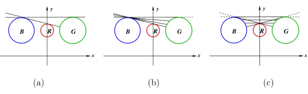
2.1 Some of the (a) vertices, (b) edges, and (c) faces of the 2D visibility complex of discs B, R, and G. . . 15 2.2 Two directed, rotating tangent lines of object R in (a) Cartesian space,
and (b) their dual representation in polar coordinates. . . 16 2.3 (a) and (c) Objects B, R, G in Cartesian space and their bitangents.
(b) and (d) Dual representation of directed rotating bitangents. . . . 17 2.4 Some of the faces of the 2D visibility complex of objects B, R, G
(shown as colored regions) and their corresponding dual representation. (a) Two faces that arise from line segments that have common occluders B, G, and their dual representations in (c); (b) one face that arises from line segments that have common occluders B, R and its dual representation in (d), and another face that arises from line segments that have common occluders R, G and its dual representation in (e). 18 2.5 The maximal free line segment corresponding to a 3D visibility complex
vertex is tangent to (a) three or (b) four objects. . . 22 2.6 The set of maximal free line segments corresponding to a 3D visibility
complex edge are tangent to (a) two or (b) three objects. . . 22 2.7 Dual representation of the 3D visibility complex of two spheres L and
R (image credits: Fredo Durand [34]). . . 23 2.8 (a) The 2D visibility skeleton vertices and arcs, computed from objects
A and B. Four vertices, labeled 1, 2, 3, 4, are shown as four blue line segments, and an arc, incident to vertices 1 and 2, is shown as a set of dashed lines. (b) The corresponding 2D visibility skeleton graph of (a); the circular cycle corresponds to the vertices whose corresponding maximal free line segments are tangent to object A in clockwise order; and the other cycle is similarly defined, based on object B. . . 27 2.9 The eight types of vertices of the 3D visibility skeleton. (a) EEEE, (b)
VEE, (c) FEE, (d) VV, (e) FF, (f) FvE, (g) FE and (h) FVV. . . 30 2.10 The degenerate case of type FvE vertex. . . 30
2.11 The four types of arcs of the 3D visibility skeleton. (a) EEE, (b) VE, (c) FE and (d) FVE. . . 31 2.12 The arcs incident to a vertex of type (a) EEEE, (b), (c) VEE, (d) VV,
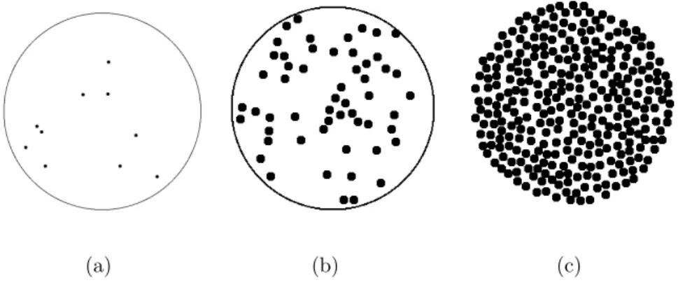
and (e), (f) FvE. . . 32 2.13 (a) T-event, (b) V-event, and (c) F-event. . . 41 3.1 Scenes of random disjoint unit discs with density as (a) 0.0025, (b) 0.1,
and (c) 0.55. . . 47 3.2 Plots of the number of oriented bitangents, memory usage, and running
time in terms of the number of unit discs, when scene density is equal to (a) 0.0025, (b) 0.005, (c) 0.025, and (d) 0.55. The unit of the memory usage is kBs, that of the running time is 10−4 seconds. . . . 50
3.3 The (a) slope and (b) y-intercept, in terms of µ, of the linear asymptote of the number of oriented bitangents (in terms of the number of discs): experimental data points and interpolations (of the square points) by
(a) 17.49
µ +5.67−19.17 µ and (b) − 4,182
µ +19, 255−23, 789 µ. The dashed
curves are the theoretical upper bounds (8(µ +4π2
µ )(n − 1) [41]) times
two since the bitangents are here oriented. . . 52 3.4 Onset of linearity in terms of the density µ: experimental data points
and their fitting by 16.77
µ + 47.55. . . 54
3.5 Number of non-oriented bitangents for density 0.0025, and an estimate of Eq. (3.1) for n > 6, 755, with, in (b), the number 4!n
2
"
of possibly obstructed bitangents and the theoretical upper bound, 8(µ +4π2
µ (n −
1)) [41] (in dashed). . . 56 3.6 Hexagonal scene model (G4). . . 58
4.1 Organization of the implementation. . . 64 4.2 Computing potential future events (marked in purple) arising from
bitangent t: (a) 4 pairs of potential T-events. (b) 4 potential V-events. (c) 4 potential F-events. . . 71 4.3 A T-event: (a) two bitangents (b) become collinear, and (c) a third
bitangent appears; (d), (e), and (f): the 2D visibility skeleton corre-sponding to (a), (b), and (c). . . 76 4.4 (a) before, (b) during, and (c) after a V-start-event, when a set of new
bitangents appears. . . 77 4.5 (a) before, (b) during, and (c) after a V-middle-event, a bitangent
changed its supporting edge. . . 78 4.6 (a) before, (b) during, and (c) after a F-event, a bitangent changed its
supporting edge. . . 78 4.7 Bitangents that are tangent to a polygon at the same or different vertices. 80
4.8 (a) Dropping z-coordinate results in different orientations of the two 2D discs: I 1 and I 2. (b) Keeping the disc orientation consistent by using the sign of (v0 · z) × (v2· z). . . 81
4.9 The 3D visibility skeleton vertices of type (a) EEEE, (b) VEE and (c) FEE that are computed from T-, V-, and F-events. Note that the maximal free line segment lies in lt, but its extent is not shown in the
figure, i.e. if it does not extend to infinity, it is blocked beyond the figure. 83 4.10 Computation of a VEE vertex, in two cases different from Figure 4.9
(b). . . 84 4.11 (a) Case (i) and (b) Case (ii) of computing an FEE vertex. . . 86 4.12 Sample scenes of (a) Scene I, (b) Scene II, (c) Scene III . . . 88 4.13 (a) One position of the sweep plane. (b) The view inside the sweep
plane. (c) The eventlist, and (d) the 2D visibility skeleton for polygons in (b). . . 89 4.14 Snapshots of visualizing the computational steps of the implementation. 90 4.15 (a) An input of ten polytopes, and the output of (b) 6 EEEE, (c) 438
VEE and (d) 85 FEE type vertices. . . 91 4.16 Running time (in seconds; 2.88 × 10⁴ seconds = 8 hours) in terms of
n, the number of edges in the scene in Suite I (µ = 0.3). . . 95 4.17 Running time (in seconds) in terms of n1.5k log k: for density (a) µ =
0.3, (b) µ = 0.05 and (c) µ = 0.01, where the polytopes have constant complexity (n/k edges) (Suite I); and (d) for density µ = 0.3, where the polytope complexity varies in the range of [4 - 24], [4 - 34], and [4 - 44] (Suite III). . . 96 4.18 Running time ratio of number type double to filtered_exact, tested
on the experiments in Suite I. . . 102 5.1 (a): Transversal ! intersects segment pq only if (! $ op) (! $ oq) ! 0.
(b-c): An illustration for the proof of Lemma 10. . . 118 5.2 Planes P1 and P2 such that P1 < P2 . . . 126
6.1 Three sample scenes of k = 50 polytopes where n/k, approximately the number of edges on each polytope, is equal to (a) 6, (b) 42, and (c) 84. The scene density µ = 0.3 in all cases. . . 137 6.2 Mean and standard deviation of the number of computed skeleton
ver-tices on ten scenes for each type of scene. . . 139 6.3 Suite I (µ = 0.3): total number of skeleton vertices in terms of n, the
number of edges in the scene. . . 140 6.4 Total number of skeleton vertices in terms of k2#n/k when (a) the
polytopes have a constant (n/k) number of edges (Suite I), and (b) the number k of polytopes is constant (Suite II). . . 142
6.5 Total number of skeleton vertices in terms of k2#n/k for polytope
complexity (n/k edges) varying in the range of [4 - 24], [4 - 34], and [4 - 44] (Suite III). . . 143 6.6 The number of vertices in terms of k2#n/k as tested on Suite I (k
polytopes having a constant, n/k, number of edges; µ = 0.3). . . 143 6.7 Number of (a) VEE, (b) FEE vertices in terms of number of EEEE
vertices (Suite I, µ = 0.3). . . 146 6.8 Number of (a) VEE, (B) FEE vertices in terms of #n/k (Suite II). . 147 6.9 Error percentage of computed skeleton vertices when using number
type double versus filtered_exact (Suite I). . . 147 7.1 Scene representing a shelf in a room with a fluorescent light on the
ceiling. The black and white regions represent the umbra and full light regions. The union of the light and dark grey regions corresponds to the penumbra. The dark gray shape represents a portion of the penumbra limited by the trace of FE arcs. In this region, the visible portion of the light source does not exceed about 40%. The schema on the right represents a section through the middle of the scene. The points a are at the boundary of umbra, and the points c are at the boundary of the penumbra. The points b are on the maximal free line segments corresponding to an arc FE involving a face of the blocker. From a to b, the percentage of the light source that is visible increases linearly from 0% to about 40%, and from b to c, it increases linearly from about 40% to 100%. Since the light grey region can be made arbitrarily large by moving the light source closer to the blocker, the trace of the FE arcs on the floor corresponds to a discontinuity of the derivative in the percentage of visible area of the light source. . . 153 7.2 The possible computational relations among the types of 3D visibility
skeleton vertices. . . 157 7.3 The value of each of the free line segments is defined by a linear function
on its intersection with the plane H. . . 161 7.4 The intersections with H of free line segments on the two VE arcs on
each side of a degenerate FvE vertex move in opposite directions. . . 162 7.5 The intersections with H of free line segments on the two FE arcs on
each side of a non-degenerate FvE vertex move in opposite directions. 162 7.6 The silhouette of the polytope from v projected on H is inside the
cone of the projected constraint edges. If the constraint edges are in the half-plane u" · x " 0, so is the polytope. . . 164
7.7 (a) Bird’s eye view and (b) 3D view of degenerate FvE vertices whose supports are polytope edge e and two sequences of faces incident to v, starting from e1 and e2, which create VE arcs with v". . . 168
7.8 When the polytope edge e intersects with the polyhedral cone of the faces incident to v, the two sequences of faces that are supports of degenerate FvE vertices turn in opposite directions until they meet, which indicates a non-degenerate FvE vertex. . . 169 7.9 In some configurations, a sequence of VE arcs may contain degenerate
FvE vertices only, with a non-degenerate FvE vertex at each end. . . . 169 7.10 (a) Three polytopes admit vertices of type VEE but not vertices of
FEE. (b) Three polytopes admit vertices of type FEE but not vertices of type VEE. (c) A cross section of (b) as indicated by the red line segment. . . 175
2.1 Number of each type of skeleton arc incident to each type of skeleton vertex. . . 33 4.1 Experimental results reported in [34, 36], on a 195Mhz R10000 SGI
Onyx2 (taken from [34]). . . 98 4.2 Experimental results for three pairs of input scenes with the number
of polytope faces approximately 450, 750, and 1000. . . 99 4.3 Running time (in seconds) in terms of number type: double, filtered_exact,
and CORE, as well as the ratio of filtered_exact and CORE to double, for four input scenes. . . 101 5.1 Percentages of failure of the degree 168 and degree 3 predicates using
double-precision floating-point interval-arithmetic, for " varying from 10−12 to 10−2. . . . 131
Introduction
Visibility problems arise commonly in areas such as computer graphics, computer vision, and robotics. In computer graphics, visibility problems have been studied for about four decades. Since the earliest problems such as visible surface determina-tion [98], or occlusion culling [21], visibility has been always an important problem in computer graphics. In computer vision, visibility is involved in problems such as object reconstruction [86, 97], or sensor placement [99]. In robotics, it is involved in problems such as motion planning [68], or robots self-localization [31].
Given a set of objects in the Euclidean space, two points in the space are mutually visible if the line segment connecting them is not blocked by any objects. Visibility problems typically address queries on whether the points or objects of interest are visible to each other. The nature of the problem implies that the study of the visibility problem is essentially the study of the sets of lines that are related to the queried objects.
Based on the set of lines that are involved in the visibility queries, the visibility 1
problem can be classified as visibility from a point, a line segment, a polygon, a region, or global visibility [11]. Global visibility addresses the visibility between any pair of given objects.
Visibility queries from a point are relatively easy to handle and well understood. Typical problems related to these types of queries are ray shooting [7], visible sur-face determination [24, 30, 42, 98], and computing shadows cast by a point light source [101, 104]. Efficient and practical algorithms and data structures, such as ray tracing [101], Z-buffer [17, 18], binary space partitioning (BSP) tree [10, 43] have been developed to solve these problems, and some of them even have hardware implemen-tations [17, 18].
However, when the visibility queries do not involve points, as in the problem of global illumination [51, 58], little is known. In particular there exists no solution for determining exactly and efficiently, in a 3D polygonal scene where polygons represent faces of objects, whether two given triangles see each other, or for determining the umbra cast by a polygonal light source. This situation suggests that the problem of global visibility is a hard one. Data structures such as the visibility complex [34, 85] and the visibility skeleton [36] have been proposed to deal with global visibility.
The visibility complex is a data structure that is designed to encode global visibility information. Roughly speaking, this data structure partitions the space of maximal free line segments into connected components of segments that touch the same objects. This data structure was initially proposed in 2D by Pocchiola and Vegter [85]. This 2D version has been extensively studied [6, 54, 84, 91], and further applied in graphics rendering [20, 77]. Later on, Durand et al. [34, 38] extended the study of the 2D
visibility complex to 3D. They introduced the 3D visibility skeleton data structure, which is a simplified version of the 3D visibility complex, that includes only partial information, i.e. the zero- and one-dimensional cells of the visibility complex.
Durand et al. applied the 3D visibility skeleton data structure to global illumi-nation computation [34, 36, 37]. In their application, the input scene and the light source are modeled as 3D polygons lying on the surfaces of the objects. They compute the 3D visibility skeleton data structure through systematic brute force examination of combinations of the vertices and edges of the input (see Section 2.2.2 for details). In addition, they use various heuristics to speed up the computation. This application produces images with high quality shadow boundaries.
Despite their positive results, the work of Durand et al. also shows some drawbacks. First, their algorithm is not efficient because it is based on a brute force enumeration, and thus has worst-case time complexity Θ(n5), where n is the total complexity of
all the input polygons. Although the observed running time complexity, improved by the heuristics, is Θ(n2.5), it is still relatively high for practical use. Second, the
worst-case size complexity of the 3D visibility skeleton is Θ(n4) in the model used
by Durand et al. , which can easily reach the memory limit of present day machines, and thus restricts the use of this data structure to small input scenes. Third, their implementation is not robust and its use requires a great deal of time-consuming human intervention to remove degeneracies from realistic scenes. As a result, the largest test scene they report contains less than 1500 polygons [34]. The 3D visibility skeleton data structure has since been often stated as impractical to use given its large size, high order complexity and robustness issues [23, 67, 70, 74, 92]. In consequence,
this data structure has not gained wide use in practical applications.
On the other hand, the empirical work [34, 36] conducted by Durand et al. reported that the Θ(n4) worst-case bound is pessimistic, except for some unrealistically
con-trived scenes. On the basis of their preliminary experiments, the observed growth of the 3D visibility skeleton appears to be quadratic in the size of the input scene.
Motivated by the preliminary results of Durand et al. , more theoretical research has recently been done to study the size of the 3D visibility skeleton in various as-pects. Bronnimann et al. [14] studied the dependence of the size of the 3D visibility skeleton on the number of polytopes rather than on the total number of edges alone. They found that, when considering the inputs as k polytopes with n edges in total, the worst-case size complexity is Θ(n2k2). Glisse [48] took into account the
worst-case average silhouette size of the polytopes. He obtained a slightly better bound of O(nk3h), where h ∈ O(n/k) is the maximum size of the silhouettes of each of
the polytopes, which could be assumed to be in O(#n/k) under some reasonable assumptions. Devillers et al. [27] studied the expected size of the 3D visibility skele-ton. When considering a simple case, e.g., the input consists of unit balls that are randomly distributed inside a great sphere, they show that the expected size is linear; and when extending the results to convex disjoint polytopes with bounded aspect ra-tio and constant complexity, they show that the expected size is linear for polytopes that are sufficiently inside the great sphere, and quadratic for polytopes that are near the boundary of the great sphere.
Although much research has been done on the theoretical aspects of the size of the 3D visibility skeleton, the problem of estimating its actual size in practice with
reasonably large input scenes has remained open. The main reason for this has been the lack of a robust and efficient implementation for conducting the research.
One of the two main goals of this thesis is to provide a robust and efficient im-plementation to enable empirical studies of the 3D visibility skeleton. The second goal is then to use the implementation to investigate when the 3D visibility skeleton data structure can be of practical interest. For this reason, we study the expected size experimentally, and determine whether the theoretically proven expected linear bound for scenes consisting of spheres also holds for polytopal scenes.
Contributions of this thesis
We first provide a systematic experimental study of the expected size of the 2D visibility skeleton. This is a simpler case than 3D, and there exists software to conduct our experiments. More importantly, analogous to the theoretical result in 3D [27], the expected size of the 2D visibility skeleton on the input of unit discs is known to be linear [41]. Thus, observing a linear behavior in 2D experiments would validate the motivation for our research in 3D. Our experimental results not only confirm the asymptotic linear behavior of the 2D visibility skeleton as a function of the number of unit discs in the input, but also provide an estimation, for a range of different fixed scene densities of discs, of the slope and y-intercept of the linear asymptote. We also estimate the onset, in terms of the number of discs, of the linear behavior.
In the 3D case, we focus on studying a 3D visibility skeleton defined by visual event surfaces, and name it as a succinct 3D visibility skeleton. A skeleton thus defined is a subset of the skeleton defined by Durand et al. [34, 36], and its size is about 50% to 75% smaller [25, 26]. The reason that we study the succinct visibility
skeleton is because it is the main interest of our research. As a recent result shows, this smaller size data structure can be used to compute direct shadow boundaries cast by polytope light source [25, 26]. Furthermore, as we will show in Chapter 7, we can compute the remaining vertices of the full skeleton from this succinct one efficiently. We start with an implementation of a sweep algorithm which was initially intro-duced by Goaoc [50]. This algorithm takes as input a set of disjoint convex polytopes in arbitrary positions, and outputs the vertices of the 3D visibility skeleton. The running time of this algorithm is O(n2k2log n), where k is the number of input
poly-topes and n is the number of polytope edges. We recall the brute force algorithm has running time Θ(n5) where n is the total number of edges of the input [34].
Slightly different from the sweep algorithm, our implementation takes as input any set of convex polytopes and either outputs the skeleton vertices, or reports that the polytopes are not in general position. By polytopes in general position, it is meant that, for example, no four polytope vertices are coplanar, and no two polytope edges are parallel. To the best of our knowledge, there exists no implementation of the 3D visibility skeleton that handles degeneracies. Our implementation represents an improvement in the sense that we systematically detect and report all degeneracies although the code to handle them remains unwritten. Moreover, our implementation computes the skeleton vertices but does not build the 3D visibility skeleton itself, as the focus of this thesis is on analyzing the size of this data structure. On the other hand, we will propose, in Chapter 7, another method for computing the skeleton from a subset of the vertices.
com-putational efficiency. A predicate is a function that returns a value from a discrete set; typically a geometric predicate returns answers such as "inside", "outside", or "on the boundary of" a geometric object, and it is typically determined by the evaluation of the sign ("positive", "negative" or "equal 0") of an expression. Evaluating a predi-cate is often more efficient than computing the exact numerical result of the function that represents the predicate. In our implementation, most of the computational pro-cedures involve the evaluation of a sequence of predicates such as orientation, which determines the orientation of four ordered 3D points, or compare_xy, which compares the lexicographical order of two 3D points.
Our implementation addresses robustness issues by the choice of number type. We implemented all predicates using the CGAL Filtered_exact number type templated with CGAL interval arithmetic (based on double number type) and the CORE li-brary [22]. Using Filtered_exact number type allows evaluation of the predicates by first using interval arithmetic, and only if this fails, using the CORE exact num-ber type. This ensures that all the predicates are evaluated correctly, and relatively efficiently.
Several predicates that are required by the algorithm have quite high algebraic degrees; this is the case, for example, of those that determine whether four segments admit a line transversal, or those that compare two positions of a sweep plane as it rotates about a line. Since high algebraic degrees may cause an implementation to be prone to errors when using fixed-precision floating-point arithmetic, and may require more memory space and computation time when using exact representation, it is important to study the degree of the predicates. We show that, in the current
implementation, the algebraic degree of the predicate that is used to compare the positions of two sweep planes can be as high as 168. We also show that the degree of these predicates can be decreased to 144 by modifying the current implementation. Finally, we offer some experimental results in this study to show the actual angular separation of two sweep planes that causes the failure of the algebraic degree 168 predicate when using fixed-precision interval-arithmetic.
We use our implementation to conduct experiments on k disjoint polytopes of size n/k on average, with vertices on unit spheres randomly distributed with fixed densities in a given (spherical) universe. We perform these experiments for (i) up to 230 polytopes with up to 1 700 edges and (ii) up to 130 polytopes with up to 9 000 edges. These experiments show that the number of vertices of the succinct visibility skeleton is roughly C k√nk, where the observed constant C varies with scene density but remains small (less than 5 in our setting).
This is the first experimentally determined asymptotic estimate of the size of the succinct 3D visibility skeleton for reasonably large n and expressed in terms of both n and k. The results show that the size of the succinct 3D visibility skeleton may be sub-quadratic; in particular, they show a sub-linear growth in n and a sub-quadratic growth in k. Assuming that the size of the silhouette of a polytope on n/k vertices is O(#n/k), our results suggest that we may express the size of the succinct visibility skeleton as a function that is linear in the size of the silhouette and quadratic in the number of polytopes; that is, the number of polytope vertices in the scene impacts the size of the succinct visibility skeleton only insofar as it increases the size of the silhouettes. Finally, our results indicate that there is no large constant hidden in the
big-O notation expressions for the size of the succinct 3D visibility skeleton.
Finally, we prove that the knowledge of the succinct 3D visibility skeleton (i.e., the visibility skeleton defined by visual events) is necessary and sufficient to compute the full skeleton (defined by Durand et al. ), in part or in whole, in almost linear time in the number of vertices computed.
As we discussed before, the visibility skeleton data structure has been used in graphics rendering in both 2D [20, 77] and 3D [33, 34, 36, 37]. While its size may appear to be an impediment to further applications, the detailed experimental studies of its size that we present in this thesis, together with the theoretical results, can provide a good reference for those who wish to use this data structure in their own applications.
In the rest of this thesis, we will present our detailed studies and results. We first provide some background and introduce related work in Chapter 2. We describe our experimental study of the size of the 2D visibility skeleton in Chapter 3. For the study of the 3D visibility skeleton, we present the details of our implementation in Chapter 4, the study of algebraic degree of the predicates that are involved in our implementation in Chapter 5, and the experimental study of the size of the skeleton defined by visual event surfaces in Chapter 6. Chapter 7 presents a method to efficiently compute the full 3D visibility skeleton from the one defined by visual event surfaces. Chapter 8 concludes with a summary of the main results and a discussion of possible future work.
Background and Related Work
In this chapter, we provide the background material needed for the rest of the the-sis, and also, we review the relevant literature. The chapter introduces the concept of the visibility complex (in Section 2.1) and the visibility skeleton (in Section 2.2), and describes the sweep algorithm (in Section 2.3) that is the basis of our implementation. The relevant literature is reviewed in each of these sections.
2.1
The Visibility Complex
Visibility computations are central in applications of computer graphics, robotics, and motion planning. Methods of reducing the expenses of these computations have been actively studied. The visibility complex, a data structure that encodes the visibility information, has been proposed to meet this need. Roughly speaking, this data structure is a partition of the space of maximal free line segments into connected components of segments that touch (i.e., are tangent to, or are blocked by) the same
objects. In comparison with previously defined similar data structures, the visibility graph for example [46], this data structure has certain advantages in that it encodes global visibility information.
The visibility complex data structure was initially proposed by Pocchiola and Vegter as a data structure encoding visibility information of a scene in two dimen-sions [85]. In 2D, the visibility complex has been extensively studied [84, 91, 54, 6], including some of its application for rendering [77, 20]. Durand et al. [34, 38] initiated the study of the visibility complex in three dimensions. Various algorithms have been studied to compute this data structure [35, 62]; however, due to its size and time complexity, applications are so far limited to the use of a simplified version, called the 3D visibility skeleton, which we will describe in Section 2.2.
We introduce the 2D and 3D visibility complex in the following two subsections.
2.1.1
The 2D Visibility Complex
Introduction
As we noted before, the 2D visibility complex was initially introduced by Pocchi-ola and Vegter [85]. We review this data structure based on their work [85]. The description of the visibility complex we give here is more intuitive though less formal than in [85].
As in the spirit of Pocchiola and Vegter [85], we limit the 2D objects to convex disjoint open sets in general position. Additionally, there is a large circle at infinity enclosing all other objects.1
The free space is thus defined as the complementary
1
Note that this large circle is not part of the input objects. Its functionality is to ensure that each extremity of any maximal free line segment is on some object.
space, with respect to the enclosing circle, of the union of all the objects. A maximal free line segment is a line segment that is maximal with respect to the inclusion in this free space. A set of maximal free line segments is connected if, roughly speaking, each segment can move continuously, within the set, to the others. More formally, a connected set of maximal free line segments consists of either bounded line segments, half-lines, or lines. In the case of bounded line segments, each line segment is defined by two points in R2, and can be parameterized by a point in R4. Such a set of maximal
free line segments is connected if the set of corresponding points in R4 is connected.
Similarly, a half-line can be parameterized by a point and a direction, and a line can be parameterized by a point in Plücker space.
The 2D visibility complex thus defined is a cell complex [85].2
All the maximal free line segments that are grouped into the same cell (component) agree on which objects they touch. Furthermore, the line segments in the same cell have 0-, 1- or 2-degrees of freedom, and hence these cells are called vertices, edges, and faces respectively.
• vertices. Each vertex of the 2D visibility complex corresponds to a maximal free line segment that is tangent to two objects. Such a line segment has 0-degrees of freedom with respect to that property. Figure 2.1 (a) illustrates two such vertices.
2
A cell complex, or CW-complex, is, at first sight, a partition of the space into cells of various dimensions that are homeomorphic to open balls such that the boundary of any cell (defined as the image, through the homeomorphism, of the boundary of the corresponding ball) is the union of a finite collection of cells of smaller dimensions. More precisely, quoting [102] (see also [56]), for each n-dimensional open cell C in the partition of the space X, there exists a continuous map f from the n-dimensional closed ball to X such that (i) the restriction of f to the interior of the closed ball is a homeomorphism onto the cell C, and (ii) the image of the boundary of the closed ball is contained in a finite union of elements of the partition whose cell dimension is less than n; moreover, (iii) a subset of X is closed if and only it meets the closure of each cell in a closed set.
• edges. Each edge of the 2D visibility complex corresponds to a maximal con-nected set of maximal free line segments that are all tangent to exactly one and the same object. This implies that the endpoints of these segments all lie on the same pair of objects or at infinity. We note that the edge thus defined does not contain their endpoints. Such a maximal free line segment has 1-degree of freedom with respect to these properties. Each edge of the complex is incident to two vertices of the complex. Here we say that an edge is incident to a vertex if the line segment corresponding to a vertex contains a line segment that is a limit of line segments that give rise to the edge. For example, Figure 2.1 (b) shows a component of line segments that are tangent to B and blocked by G. These line segments have 1-degree of freedom with respect to these properties, and thus give rise to an edge of the complex. That edge is incident to the vertex arising from a line segment tangent to B and R and blocked by G, and another vertex arising from a line segment tangent to B and G. Note that in Figure 2.1 (b), the solid line segment tangent to B and G represents a limit of the segments defining the edge. This line segment, together with its extension, illustrated as dotted, is a line that represents the vertex that the edge is incident to. Note also that the other edges and vertices arising from the objects B, R and G are not illustrated in Figure 2.1 (b). Finally, we note that in the work of Pocchiola and Vegter [85], the visibility complex is formally defined in a quotient space, such that a line segment corresponding to the limit of an edge is identified to a line segment corresponding to a vertex.
that are blocked by the same two common objects; thus each such line segment has 2-degrees of freedom with respect to this property. A face is incident to an edge (or a vertex) if the line segments in the component that gives rise to the face can be continuously moved within that component to the line segments that give rise to the edge (or the vertex). For example, Figure 2.1 (c) shows a component of line segments that are blocked by B and G, and that have 2-degrees of freedom with respect to this property; thus they give rise to a face of the complex. That face is incident to vertices that are arising from line segments tangent to B and G, B and R, R and G; and edges that are arising from line segments tangent to B and blocked by G, tangent to G and blocked by B, tangent to R and blocked by B and G. The vertices and edges incident to a face form a cycle.
y x B R G y x B R G y x B R G (a) (b) (c)
Figure 2.1. Some of the (a) vertices, (b) edges, and (c) faces of the 2D visibility complex of discs B, R, and G.
In the visibility complex, the dimension of a cell corresponds to the number of degrees of freedom of the maximal free line segment giving rise to the cell. As previ-ously noted, in the 2D visibility complex, a vertex is a 0D cell, an edge is a 1D cell, and a face is a 2D cell.
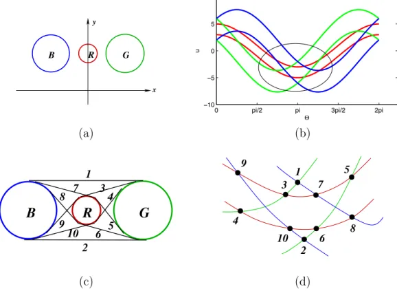
The 2D visibility complex can be better viewed in a dual representation that is expressed in the polar coordinates of a directed line. Here a directed line y cos(θ) − x sin(θ) = u is expressed by polar coordinates (θ, u), where θ is the angle the line forms with the x-axis measured in the counterclockwise sense, and u is the signed distance of the line to the origin. Given an object, for example, disc R in Figure 2.2 (a), and an angle θ, there are two directed lines tangent to the object. As θ varies from 0 to 2π, the motion of the two directed lines that are tangent to disc R appear as two sinusoidal waves in the (θ, u) dual representation, as in Figure 2.2 (b).
These two sinusoidal waves partition the line space into three cells, namely, the space in between the two sinusoidal waves, called cell I, the space that is above the two sinusoidal waves, called cell II, and the space that is below the two sinusoidal waves, called cell III. Any (oriented) line that belongs to cell I intersects disc R, whereas any (oriented) line that belongs to cell II (respectively cell III) leaves disc R to its left (respectively right), and any line on the cell boundary is tangent to disc R.
θ u
y
x
R
0 pi/2 pi 3pi/2 2pi
−5 0 5 Θ u cell I cell II cell III (a) (b)
Figure 2.2. Two directed, rotating tangent lines of object R in (a) Cartesian space, and (b) their dual representation in polar coordinates.
dual representation appear as several pairs of sinusoidal waves (Figure 2.3). These sinusoidal waves partition the dual space into cells, such that the vertices of the visibility complex map to the intersections of two sinusoidal waves, the edges of the visibility complex map to the curved segments on the sinusoidal waves that are delimited by two consecutive vertices, and the faces of the visibility complex map to the cells that are delimited by a chain of vertices and edges.
B
y
x
G R
0 pi/2 pi 3pi/2 2pi
−10 −5 0 5 10 Θ u (a) (b)
B
R
G
1 4 3 7 9 5 6 10 8 2 1 2 6 3 7 10 9 8 5 4 (c) (d)Figure 2.3. (a) and (c) Objects B, R, G in Cartesian space and their bitangents. (b) and (d) Dual representation of directed rotating bitangents.
Figure 2.3 (d) details the circled region in Figure 2.3 (b). Each numbered vertex in Figure 2.3 (d) has its corresponding representation in Cartesian space as shown in Figure 2.3 (c). Figure 2.4 illustrates some of the faces of this example scene in Cartesian space and in the corresponding dual representation.
B
R
G
1 3 7 6 10 2B
R
G
1 4 3 7 9 5 6 10 8 2 (a) (b) 1 2 3 6 10 7 9 8 4 5 10 7 9 8 6 3 4 5 (c) (d) (e)Figure 2.4. Some of the faces of the 2D visibility complex of objects B, R, G (shown as colored regions) and their corresponding dual representation. (a) Two faces that arise from line segments that have common occluders B, G, and their dual representations in (c); (b) one face that arises from line segments that have common occluders B, R and its dual representation in (d), and another face that arises from line segments that have common occluders R, G and its dual representation in (e).
Algorithms and Implementations
Pocchiola and Vegter presented a greedy flip algorithm to compute the 2D visibility complex data structure of an input set of n disjoint (or touching) convex objects of constant complexity. The algorithm runs in O(n log n+k) time, where n is the number of objects and k is the complexity of the 2D visibility complex [84, 85]. The space complexity for the computation is linear in k in [85], and improved to be linear in n in [84]. The size of k is Θ(n2) in the worst case and Ω(n) in all cases. Briefly,
the algorithm constructs a pseudo-triangulation of the input objects using their free bitangents. Starting from a unit vector at angle 0, they then rotate the unit vector up to angle π. The bitangents that have the same angle as the rotating vector are flipped, and the pseudo-triangulation is updated accordingly.
Angelier and Pocchiola later on implemented the greedy flip algorithm [5]. In particular, they improved the flip operation in the algorithm to constant computa-tion time per flip by means of a “sum of squares” theorem [6]. The implementacomputa-tion takes convex disjoint discs as input, as allowed by the algorithm [84, 85], and it han-dles objects such as points, segments, and convex polygons, by applying symbolic perturbation to ensure these objects satisfy a smooth boundary condition.
Before Angelier and Pocchiola, Rivière implemented a sweep algorithm to compute the visibility complex of convex disjoint polygons [90]. While this implementation has O(n log n + k) running time and O(n) space, where n is the total complexity of input polygons and k is the size of the computed 2D visibility complex. Like the greedy flip algorithm, the author shows through experimental results that his implementation is efficient in practice, as the constant of the big Oh notation is small.
Rivière also gave a method for updating the visibility complex in a dynamic polyg-onal scene in O(log n) time at each step, after O(k log n) time precomputation of this data structure [91].
Applications
The 2D visibility complex has various applications.
vertices of the visibility complex are used to compute the discontinuity mesh, and the faces of the visibility complex are used to compute the form factor. Computing radiosity this way can avoid much redundant computation compared to the traditional method.
In [20], Cho and Forsyth use the 2D visibility complex in ray tracing. Two basic properties that they use to render images efficiently are: 1) within the same cell of the visibility complex, the set of rays encounter the same set of objects; 2) radially sweeping a ray in primary, Cartesian space is equivalent to walking along a line segment in the dual space. Their experimental results show that their ray tracer, which uses the 2D visibility complex, is about 3.5 times faster than the conventional ray tracer.
Moreover, Rivière [91] and Hall-Holt [54] make use of the visibility complex data structure to design algorithms for maintaining views in scenes in which the view point moves, but objects are fixed.
2.1.2
The 3D Visibility Complex
Introduction
We introduce the 3D visibility complex based on the work of Durand et al. [34, 38] as it was initially presented.
The 3D visibility complex is an extension of the concept of the 2D visibility com-plex. However the 3D visibility complex is not a cell complex since some of the cells are not contractible to a point. Moreover a line in 3D has four degrees of freedom, and therefore the cells that partition the 3D line space can have higher dimension
than the cells in the 2D case.
In what follows, we define the cells of the 3D visibility complex. We note that the concept of each cell is based on smooth objects that are in general position. We say 3D objects are in general position when free line segments tangent to any n of them have 4 − n degrees of freedom with respect to that property, for 0 ! n ! 4.
• a vertex corresponds to a maximal free line segment that is tangent to three or four objects that are in general position (Figure 2.5). In the case of three objects, the maximal free line segment lies on a plane that is tangent to two objects. Such line segment has 0-degrees of freedom. A vertex is a 0D cell. • an edge corresponds to a set of maximal free line segments that are tangent
to two or three objects that are in general position, and form one connected component (Figure 2.6). In the case of two objects, the set of maximal free line segments lie on a set of planes that are tangent to the two objects. In such a set, each line segment has 1 degree of freedom. An edge is a 1D cell.
• a bitangency (respectively tangency) face corresponds to a set of maximal free line segments that are tangent to two (respectively one) objects that are in general position, and form one connected component. In such a set, each line segment has 2 (respectively 3) degree(s) of freedom. A bitangency (respectively tangency) face is a 2D (respectively 3D) cell.
• a face corresponds to a set of line segments that are being occluded by the same two objects, form one connected component. Each of the line segments in such a set has 4-degrees of freedom. A face is a 4D cell.
(a) (b)
Figure 2.5. The maximal free line segment corresponding to a 3D visibility complex vertex is tangent to (a) three or (b) four objects.
(a) (b)
Figure 2.6. The set of maximal free line segments corresponding to a 3D visibility complex edge are tangent to (a) two or (b) three objects.
In the dual representation, a line is expressed by the polar coordinates (θ, ϕ, u, v) where θ is the azimuth and ϕ is the elevation. In order to define u and v, we consider the plane perpendicular to the line and passing through the origin. We chose an orthogonal coordinate system u, v on this plane such that the u axis is perpendicular to the y axis. The values u and v in the dual representation are then the coordinates in this system of the intersection of the line with the plane. This definition does not allow representation of a line parallel to the y axis, but the definition is sufficient for many purposes.
Given a sphere L, as in Figure 2.7, and a direction (θ, ϕ), a set of lines that are tangent to sphere L appear as a circle in the dual representation. When varying θ from 0 to π, the tangency face of L appears as a curvy tube L in the dual. Furthermore,
if considering the fourth dimension ϕ as similar to a time t, then varying ϕ from 0 to π can be described as the morphing motion of the curvy tube. As in Figure 2.7, this morphing curvy tube L is the dual representation of the tangency face of sphere L. It partitions the line space into intersecting, tangent, and non-intersecting lines to sphere L, depending on whether a given line in its dual representation is inside, on, or outside the curvy tube.
Figure 2.7. Dual representation of the 3D visibility complex of two spheres L and R (image credits: Fredo Durand [34]).
another morphing curvy tube R. The intersection volume of these two curvy tubes represents a set of lines that intersect both spheres. In particular, when the surfaces of these two tubes intersect, it results in a 3D curve in the (θ, u, v) coordinate system for a given ϕ cross-section, and represents a bitangency face. For convenience we call this curve a bitangency curve. When two such bitangency curves intersect, their intersection represents an edge. We call this intersection an edge curve. This edge curve appears as one point for a given ϕ in (θ, u, v) coordinates, and appears as a curve when ϕ varies. Note that the extremities of the bitangency curve, at which the value of θ is minimal or maximal, also result in an edge curve. Such an edge curve corresponds to a set of lines that lie on a set of planes that are tangent to two spheres. When two edge curves intersect at some ϕ, this intersection defines a unique 4-tuple (θ, ϕ, u, v) of coordinates, which corresponds to a line tangent to four objects in 3D Cartesian space, and represents a vertex of the 3D visibility complex.
Algorithms and Implementations
Durand et al. presented a double sweep algorithm to compute the 3D visibility complex of an input scene consisting of 3D polygons or smooth objects [35]. The running time of this algorithm is O((v + n3) log n) where n is the complexity of the
input, and v is the number of the vertices of the 3D visibility complex, which is Ω(n) and O(n4). Moreover, the authors emphasized that v is much less than O(n4) in
experimental results. Hence the running time of the algorithm in practice appears to be less than the worst case theoretical running time of O(n4log n). Nevertheless, due
to have been done.
Goaoc presented a sweep algorithm to compute the 0D and 1D cells of the visibility complex (see Section 2.3 for detail) [50]. Based on Goaoc’s sweep algorithm, Hornus presented another sweep algorithm to compute the 3D visibility complex of an input scene consisting of disjoint convex polytopes [62]. The running time of this algorithm is O(n2k2log n), where k is the number of polytopes and n is the number of edges. The
author claims that this is the first seemingly implementable algorithm for computing the 3D visibility complex, although there is no implementation available yet.
Applications
The 3D visibility complex was first proposed for applications such as global il-lumination, kinetic visibility, etc. However, it has so far not been used, due to its complicated data structure.
Instead, a simplified version of the 3D visibility complex, that is, the 3D visibility skeleton, was used for global illumination and has attracted more research attention.
In the next subsection, we introduce the visibility skeleton data structure.
2.2
The Visibility Skeleton
The visibility skeleton data structure is a simplified version of the visibility com-plex that consists of only the 0D and 1D cells of the visibility comcom-plex. This data structure was first introduced in 3D by Durand et al. [34, 36] and used in shadow boundary computation [32, 34, 36]. The application of this data structure was suc-cessful but limited to only small input scenes, since the practical running time
com-plexity of the algorithm that is used to compute it is relatively high (O(n2.5)), and
the worst-case size complexity of this data structure is large (O(n4)). These apparent
limitations have motivated researchers to study its average size and to design efficient algorithms to compute it. The ongoing research of others in this area will be intro-duced later in this chapter, as indeed, the main part of this thesis also studies the 3D visibility skeleton.
The 2D visibility skeleton data structure was later introduced by Goaoc [50] when designing a sweep algorithm to compute the 3D visibility skeleton.
In the visibility skeleton data structure, a 0D cell is called a vertex and a 1D cell is called an arc. Recall that, in the visibility complex data structure, the 0D cell corresponds to a maximal free line segment that has 0-degrees of freedom; and the 1D cell corresponds to a connected set of maximal free line segments that have 1-degree of freedom. This concept holds in the visibility skeleton data structure as well. Moreover, the incidence relation of vertices and arcs is encoded into a graph, namely, the visibility skeleton graph. We will introduce this data structure in 2D and 3D in detail in the next two sections.
2.2.1
The 2D Visibility Skeleton
We introduce this data structure based on the work of Goaoc [50], but limit ourselves to the case where objects are in general position. By general position, we mean that no three vertices are collinear.
1
4
3
2
A
B
4 1 2 3 (a) (b)Figure 2.8. (a) The 2D visibility skeleton vertices and arcs, computed from objects A and B. Four vertices, labeled 1, 2, 3, 4, are shown as four blue line segments, and an arc, incident to vertices 1 and 2, is shown as a set of dashed lines. (b) The corresponding 2D visibility skeleton graph of (a); the circular cycle corresponds to the vertices whose corresponding maximal free line segments are tangent to object A in clockwise order; and the other cycle is similarly defined, based on object B.
2D Visibility Skeleton Vertices and Arcs
In 2D, there is only one type of vertex and one type of arc. Each vertex corresponds to a maximal free bitangent that is tangent to two objects. Each arc corresponds to a set of connected maximal free line segments that are tangent to one given object, and possibly blocked by 0, 1, or 2 other objects. A graphical illustration of the 2D visibility skeleton vertices and arcs is shown in Figure 2.8 (a).
The 2D Visibility Skeleton Graph
In the 2D visibility skeleton graph, each vertex is incident to four arcs, and each arc is incident to two vertices. In particular, the corresponding maximal free line segments of each arc, and its two incident vertices, are tangent to a common object. An example graph is shown in Figure 2.8 (b), which is computed from the two polygons A and B, as shown in Figure 2.8 (a).
follows. Two adjacent vertices of the graph correspond to two maximal free line segments tangent to a common object. The free line segments are ordered clockwise, and the arc incident to both vertices is oriented accordingly. As in Figure 2.8, the circular cycle of directed arcs gives the ordering of the 4 bitangents around polygon A; the cycle of the remaining directed arcs gives the ordering of the 4 bitangents around polygon B.
Algorithms, Implementations, and Applications
As we mentioned at the beginning of this section, the 2D visibility skeleton con-cept was arose during the design of a sweep algorithm to compute the 3D visibility skeleton [50]. In [50], Goaoc uses the same algorithm [84] (presented by Pocchiola and Vegter) and implementation [5] (implemented by Angelier and Pocchiola) of the 2D visibility complex (see Section 2.1 for detail), but discards the information about the faces (2D cells).
2.2.2
The 3D Visibility Skeleton
Unlike the 2D visibility skeleton, the nature of the 3D visibility skeleton varies with the nature of the input objects, i.e. whether the contour of the object is smooth or not. Moreover, over the literature history, people have studied the 3D visibility skeleton according to their own research interests, and defined this data structure differently.
In this section, we first introduce this data structure using the 0D and 1D cells of the visibility complex for an input consisting of 3D polytopes, based on the work
of Durand et al. [34, 36]. Then we introduce an alternative definition that is based on visual event surfaces, based on the work of Demouth et al. [25]. Then finally, we introduce this data structure based on smooth objects.
The 3D Visibility Skeleton of a Set of Polytopes
We first make some preliminary definitions in order to explain the types of vertices and arcs of the 3D visibility skeleton of a set of polytopes.
A support vertex of a line is a polytope vertex that lies on the line. A support edge of a line is a polytope edge that intersects the line but has no endpoint on it (a support edge intersects the line at only one point of its relative interior). A support of a line is one of its support vertices or support edges. The supports of a segment are defined to be the supports of the interior of the segment; thus if a maximal free segment ends at a vertex of a polytope, this vertex is not a support. A support polytope of a line is the polytope that the support of the line lies on.
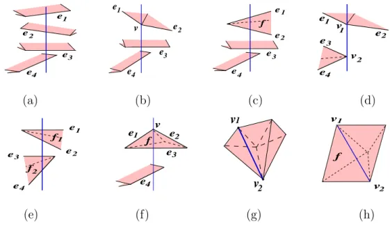
3D Visibility Skeleton Vertices. There are eight types of skeleton vertices. We define them based on [34, 36], and show graphical illustrations in Figure 2.9. Note that unless stated otherwise, no two supports will come from the same polytope. A skeleton vertex has type: EEEE if its set of supports consists of four edges; VEE if its set of supports consists of a vertex and two edges; FEE if its set of supports consists of two edges on one face, and two additional edges; VV if its set of supports consists of two vertices; FF if its set of supports consists of two edges on one face, and two edges on another face; FvE if its set of supports consists of a vertex and an edge on one face, and an edge; FE if its set of supports consists of two adjacent vertices of the
e1 e2 e3 e4 v e 1 e 2 e e4 3 2 e1 e e3 e4 f e e e e 3 4 1 2 v2 v1 (a) (b) (c) (d) f 2 1 e 4 e 3 f e e 1 2 1 e e2 e3 e 4 v f 1 2 v v f v 1 2 v (e) (f) (g) (h)
Figure 2.9. The eight types of vertices of the 3D visibility skeleton. (a) EEEE, (b) VEE, (c) FEE, (d) VV, (e) FF, (f) FvE, (g) FE and (h) FVV.
1 e2 e e4 3 e f v
Figure 2.10. The degenerate case of type FvE vertex.
same polytope; and FVV if its set of supports consists of two non-adjacent vertices on the same face of a polytope.
We note a degenerate case of the type FvE vertex, as shown in Figure 2.10. Its set of supports consists of a vertex, a face that the vertex lies on, and an additional edge. Note that in contrast to a non-degenerate FvE vertex, a degenerate FvE vertex has only one edge support. Note also that our definition differs from the discussion in [48], in which this degenerate case of an FvE vertex is not considered to generate a skeleton vertex.
e2 1 e e3 v e f e f v1 v2 (a) (b) (c) (d)
Figure 2.11. The four types of arcs of the 3D visibility skeleton. (a) EEE, (b) VE, (c) FE and (d) FVE.
It should be stressed that the maximal free line segment corresponding to a skele-ton vertex is tangent to all its support polytopes.
3D Visibility Skeleton Arcs. There are four types of skeleton arcs. We define them, based on [34, 36], as follows, and show graphical illustrations in Figure 2.11. Note that unless stated otherwise, no two supports will come from the same polytope. An arc has type: EEE if its set of supports consists of three edges; VE if its set of supports consists of a vertex and an edge; FE if its set of supports consists of two edges on one face, and one additional edge; Fv if its set of supports consists of one vertex and one edge on the same face which is not incident to it.
Again, we emphasize that the maximal free line segments corresponding to a skeleton arc are tangent to all their support polytopes.
The 3D Visibility Skeleton Graph. When the inputs are convex disjoint poly-topes in general position, each skeleton vertex is incident to three to six skeleton arcs, according to the type of the skeleton vertex; and each skeleton arc is incident to two skeleton vertices. We note that the visibility skeleton graph is not necessarily a connected graph.