Effect of fluid inertia on the orientation of a small prolate spheroid settling in turbulence

HAL Id: hal-02267471

https://hal.archives-ouvertes.fr/hal-02267471

Submitted on 19 Aug 2019

HAL is a multi-disciplinary open access

archive for the deposit and dissemination of

sci-entific research documents, whether they are

pub-lished or not. The documents may come from

teaching and research institutions in France or

abroad, or from public or private research centers.

L’archive ouverte pluridisciplinaire HAL, est

destinée au dépôt et à la diffusion de documents

scientifiques de niveau recherche, publiés ou non,

émanant des établissements d’enseignement et de

recherche français ou étrangers, des laboratoires

publics ou privés.

prolate spheroid settling in turbulence

K. Gustavsson, M Z Sheikh, D Lopez, A. Naso, A. Pumir, B Mehlig

To cite this version:

K. Gustavsson, M Z Sheikh, D Lopez, A. Naso, A. Pumir, et al.. Effect of fluid inertia on the

orientation of a small prolate spheroid settling in turbulence. New Journal of Physics, Institute of

Physics: Open Access Journals, 2019, 21 (8), pp.083008. �10.1088/1367-2630/ab3062�. �hal-02267471�

PAPER • OPEN ACCESS

Effect of fluid inertia on the orientation of a small prolate spheroid settling

in turbulence

To cite this article: K Gustavsson et al 2019 New J. Phys. 21 083008

View the article online for updates and enhancements.

PAPER

Effect of

fluid inertia on the orientation of a small prolate spheroid

settling in turbulence

1 _{Department of Physics, Gothenburg University, SE-41296 Gothenburg, Sweden}

2 _{Univ. Lyon, ENS de Lyon, Univ. Claude Bernard, CNRS, Laboratoire de Physique, F-69342, Lyon, France}

3 _{Univ. Lyon, Ecole Centrale de Lyon, Univ. Claude Bernard, CNRS, INSA de Lyon, Laboratoire de Mécanique des Fluides et d’Acoustique,}

F-69134, Ecully, France

4 _{Max-Planck Institute for Dynamics and Self-Organization, D-37077, Göttingen, Germany}

E-mail:bernhard.mehlig@physics.gu.se

Keywords: turbulence, non-spherical particles, angular dynamics, settling, ice crystals in cumulus clouds

Abstract

We study the angular dynamics of small non-spherical particles settling in a turbulent

flow, such as ice

crystals in clouds, aggregates of organic material in the oceans, or

fibres settling in turbulent pipe flow.

Most solid particles encountered in Nature are not spherical, and their orientations affect their settling

speeds, as well as their collision and aggregation rates in suspensions. Whereas the random action of

turbulent eddies favours an isotropic distribution of orientations, gravitational settling breaks the

rotational symmetry. The precise nature of the symmetry breaking, however, is subtle. We demonstrate

here that the

fluid-inertia torque plays a dominant role in the problem. As a consequence rod-like

particles tend to settle in turbulence with horizontal orientation, the more so the larger the settling

number Sv

(a dimensionless measure of the settling speed). For large Sv we determine the fluctuations

around this preferential horizontal orientation for prolate particles with arbitrary aspect ratios, assuming

small Stokes number St

(a dimensionless measure of particle inertia). Our theory is based on a statistical

model representing the turbulent velocity

fluctuations by Gaussian random functions. This overdamped

theory predicts that the orientation distribution is very narrow at large Sv, with a variance proportional

to

Sv

_{. By considering the role of particle inertia, we analyse the limitations of the overdamped theory,}

and determine its range of applicability. Our predictions are in excellent agreement with numerical

simulations of simpli

fied models of turbulent flows. Finally we contrast our results with those of an

alternative theory predicting that the orientation variance is proportional to

Sv

_{at large Sv.}

1. Introduction

The settling of particles in turbulence is important in a wide range of scientific problems. An example is the settling of small ice crystals in clouds[1]. The orientation of small ice crystals has manifestly a direct impact on

the reflection properties of electromagnetic waves (including light) from clouds [2–4], with potentially

important consequences for the albedo and the climate. In addition, it was noted that the dispersion in the orientation of identical crystals leads to differences in their settling velocities, which in turn affects the collision and aggregation rates[5,6], essential in the formation of precipitation. A second example highlighting the

significance of particles settling in turbulence is the dynamics of small aggregates of organic matter in the oceans (‘marine snow’) [7]. The interaction of settling and turbulence also affects the dynamics of swimming of

microorganisms[8–10] in the oceanographic context. A problem of industrial relevance is the wall-deposition of

fibres in a turbulent pipe flow [11].

The settling of spherical particles in turbulence has been intensively studied. Maxey and collaborators [12–14] found that turbulence increases the settling speed of small spherical particles. This pioneering work has

led to many experimental and numerical studies, using direct numerical simulation(DNS) of turbulence, and it is a question of substantial current interest[15,16]. An important question is how frequently particles collide as

OPEN ACCESS RECEIVED

31 March 2019

REVISED

6 June 2019

ACCEPTED FOR PUBLICATION

9 July 2019

PUBLISHED

5 August 2019

Original content from this work may be used under the terms of theCreative Commons Attribution 3.0 licence.

Any further distribution of this work must maintain attribution to the author(s) and the title of the work, journal citation and DOI.

they settle in turbulence[17,18]. The collision rate is influenced by spatial inhomogeneities in the

particle-number density due to the effect of particle inertia. There is substantial recent progress in understanding this two-particle problem[19–23]. The conclusion is that settling may increase or decrease spatial clustering of

spherical particles, and that it tends to decrease the relative velocities of nearby particles because settling reduces the frequencies of‘caustics’, singularities in the inertial-particle dynamics [19].

Most solid particles encountered in Nature and in Engineering are not spherical, yet less is known about the settling of non-spherical particles in turbulence, and their settling depends in an essential way on their

orientation. In afluid at rest the orientation of a slowly settling non-spherical particle is determined by weak torques induced by the convective inertia of thefluid—set in motion by the moving particle. For a single, isolated particle in a quiescentfluid this effect is well understood [24–27]: convective fluid inertia due to slip between the

particle and thefluid velocity causes non-spherical particles to settle with their broad side first. For axisymmetric rods, for example, symmetry dictates that the angular dynamics has two equilibrium orientations: either the rod is aligned with gravity(tip first) or perpendicular to gravity. At weak inertia, only the latter orientation is stable, so that the rod settles with its long edgefirst. But when there is turbulence, then turbulent vorticity and strain exert additional torques that causefluctuations in the orientations of the settling crystals [1,28].

To understand the angular motion of a non-spherical particle settling in turbulence is in general a very complex problem, because there are many dimensionless parameters to consider. There is particle shape(shape parameterΛ), and the effect of particle inertia is measured by the Stokes number St. The importance of settling is determined by Sv, a dimensionless measure of the settling speed. The significance of fluid inertia is quantified by two Reynolds numbers, the particle Reynolds numberRep(convective inertia due to slip between particle and

fluid velocity), and the shear Reynolds numberRes(convective inertia due to fluid-velocity gradients). The

nature of the turbulent velocityfluctuations is determined by the Taylor-scale Reynolds numberRel.

If the particles are so small that they just follow theflow and that any inertial corrections to the fluid torque are negligible(Rep=Res=0), then the angular dynamics of small crystals in turbulence is well understood [10,29–38]. The particle orientation responds to local vorticity and strain through Jeffery’s equation [29]. The

effect of particle inertia is straightforward to take into account[39], but the role of fluid inertia is more difficult to

describe, even in the absence of settling. In certain limiting casesfluid-inertial effects are well understood. The most important example is that of a small neutrally buoyant(Res=St) spheroid moving in a time-independent

linear shearflow, so that the centre-of-mass of the particle follows the flow (Rep=0). Neglecting inertial effects

(Res=0) and angular diffusion, the angular dynamics degenerates into a one-parameter family of marginally

stable orbits, the so-called Jeffery orbits[29]. Fluid inertia breaks this degeneracy and gives rise to certain stable

orbits[40–43]. Much less is known whenRepis not zero. Candelier, Mehlig and Magnaudet[44] recently

showed how to compute the effect of a small slip upon the force and torque on a non-spherical particle in a general linear time-independentflow, by generalising Saffman’s result [45,46] on the lift upon a small sphere in

a shearflow, valid in the limit whereRep Res 1.

The results summarised in the previous paragraph pertain to time-independentflows. Time-dependent spatially inhomogeneousflows present new challenges, and very little is known about the effect of fluid inertia for suchflows, in particular for turbulence. In some studies, therefore, effects of fluid inertia were simply neglected[5,6,47–49]. These models predict that the breaking of isotropy due to gravity causes a bias in the

orientation distribution of the settling particles, so that rods tend to settle tipfirst, parallel to gravity. For small particles it is safe to neglectRes[50]. But experiments and numerical simulations of slender particles settling in a

vortexflow [51] and in turbulence [52] show that convective inertial torques due to settling can make a

qualitative difference to the orientation distribution.

In this paper we therefore consider the effect of the convective inertial torques on the orientation of small spheroids settling in turbulence. Following[51], our model assumes that the hydrodynamic torque is

approximately given by the sum of Jeffery’s torque and the convective inertial torque in a homogeneous, time-independentflow. For nearly spherical particles this convective torque was calculated by Cox [24], and for slender

bodies by Khayat and Cox[25]. Their results were generalised to spheroids with arbitrary aspect ratios in [26].

Our goal is to analyse how the turbulent-velocityfluctuations affect the orientation distribution of a prolate spheroid settling through turbulence. We assume that the particles are small enough so that convective-inertia effects due to thefluid-velocity gradients are negligible, that inertial effects on the centre-of-mass motion are small(small St andRep), but that the settling number Sv is large enough so that the fluid-inertia torque

dominates the angular dynamics.

Wefind an approximate theory for the angular distribution of settling spheroids using a statistical model [48,53] for the turbulent fluctuations. The theory is valid for large Sv and small St, in the overdamped limit, and

its predictions are in excellent agreement with results of numerical simulations of the statistical model, and with simulations using a kinematic-simulation(KS) model [54,55] for the turbulent flow. We find that the variance

number St, and the theory determines how the pre-factor depends on the shape of the spheroid. In the slender-body limit, theSv-4_{-scaling of the variance was also found in[56] using an approach equivalent to ours.}

We contrast our results with a theory for the orientation variance derived by Klett[28] for nearly spherical

particles. This theory predicts that the variance is proportional toSv-2_{. Atfirst sight this may appear to be at}

variance with the overdamped theory, but we show that the overdamped approximation breaks down into several different regimes when particle inertia begins to matter. At very large values of Sv, when the time scale at which thefluid-velocity gradients decorrelate is the smallest time scale of the inertial dynamics, our numerical simulations show aSv-2_{-scaling, as suggested by Klett’s theory. But the theory is difficult to justify because it}

neglects particle inertia in the centre-of-mass dynamics. Our numerical simulations demonstrate that translational particle inertia has a significant effect upon the angular dynamics, indicating that it must be taken into account as soon as the overdamped approximation for the angular dynamics breaks down.

The remainder of this paper is organised as follows. In section2we describe our model: the approximate equations of motion and the statistical model for the turbulent-velocityfluctuations. In section3we show results of numerical simulations of our model. We describe how and why the results differ from those in[5,6,47–49],

and explain the intuition behind our theory for small St and large Sv. The overdamped theory is described in section4. Section5discusses the effect of particle inertia, and section6contains our conclusions as well as an outlook.

2. Model

2.1. Particle equation of motion

Newton’s equations of motion for a single non-spherical particle read:

= + = ˙ ˙ ( ) v f g x v mp p mp , p p, 1a  w =t =w  [ ( )n ] n˙ n ( ) m , . 1b t p_dd p p p

Heregis the gravitational acceleration with directiongˆ =g g , x∣ ∣ pis the position of the particle, vpits

centre-of-mass velocity, mpthe particle mass, and the dots denote time derivatives. We assume that the particle is

axisymmetric, so that its orientation is characterised by the unit vectorn along the symmetry axis of the particle. The angular velocity of the particle is denoted by wp, and ( )pn is its rotational inertia tensor per unit-mass in the

lab frame. For a spheroid, the elements of ( )pn are given by[57]

 = ^ d - +  ^= +l ^ = ^ ( ) ( )n I ( n n) I n n, I 1 a I a ( ) 5 , 2 5 , 2 ij ij i j i j p 2 2 2

where l ºa a ^is the aspect ratio of the spheroid, 2aPis the length of the symmetry axis, and 2a⊥is the

diameter of the spheroid. Prolate spheroids correspond toλ>1, whereas oblate spheroids have λ<1. The difficulty lies in computing the hydrodynamic forcef and torqueτ on the particle. In the Stokes approximation, unsteady and convective inertial effects are neglected. In this creeping-flow limit [57], the force

and torque exerted by a steadyflow upon the spheroid are linearly related to the slip velocityWºvp-u, to the

angular slip velocity wp-W, and to thefluid strain :

    t = p m W w -^ ⎡ ⎣ ⎢ ⎤ ⎦ ⎥ ⎡_⎣⎢ ⎤_⎦⎥ ⎡ ⎣ ⎢ ⎢ ⎤ ⎦ ⎥ ⎥ ( ) ( ) ( ) f u v a 6 0 0 0 . 3 0 0 p p

Hereμ is the dynamic viscosity of the fluid, º (u u xp,t)is the undisturbedfluid velocity at the particle position

xp, Wº  u 1

2 is half the vorticity of the undisturbedfluid-velocity field at the particle position, and  is the

strain-rate matrix, the symmetric part of the matrix of the undisturbedfluid-velocity gradients (its antisymmetric part is denoted by). The tensors , , andare translational and rotational resistance tensors. Their forms are determined by the shape of the particle. Equation(3) shows that the tensor  relates the hydrodynamic force_f( )0

to the slip velocity W . For an axisymmetric particle with fore-aft symmetry the tensor takes the form

d

º ^( - )+  ( )

Aij A ij n ni j A n n .i j 4

The resistance coefficientsA and A^ Pdepend on the shape of the particle. For a spheroid, they are given by[57]:

l l l b l l l b b l l l l = -- + = -- -= + -^ ( )  [( ) ] ( ) [( ) ] [ ] ( ) A 8 1 A 3 2 3 1 , 4 1 3 2 1 1 , with ln 1 1 . 5 2 2 2 2 2 2

For a sphere one has A_⊥=A_P=1, so that _f( )0 _{simplifies to the expression for Stokes force on a sphere moving}

In the creeping-flow limit, the steady slip velocity W of a spheroid subject to a gravitational forcempgis

obtained by setting the acceleration ˙vpto zero in equation(1a):

T T  t = [ ^-( - )+ - ] ( ) ( ) W 0 A nn A nn g. 6 p 1 1

Here  is the unit matrix, and tpº(2a a ^rp) (9nrf)is the particle response time in Stokes’ approximation with

kinematic viscosityν=μ/ρf,fluid-mass density ρf, and particle-mass densityρp. The slip velocity depends on

the orientationn of the particle.

For an axisymmetric particle with fore-aft symmetry, the rotational resistance tensors take the form:

 d

º ^( - )+  = ( )

Cij C ij n ni j C n ni j andHijk H0 ijl k ln n. 7

Hereòijlis the anti-symmetric Levi-Civita tensor, and we use the Einstein summation convention: repeated

indices are summed from 1 to 3. For a spheroid, the rotational resistance coefficients read [57]:

l l l b l b l l l = -- - = -= - -+ ^ ^ ^ ^    ( ) [( ) ] ( ) ( ) ( ) C a a C a a H C 8 1 9 2 1 1 , 8 1 9 1 , 1 1. 8 4 2 2 2 2 0 2 2

Expressions(3)–(8) determine the hydrodynamic force and torque in the creeping-flow limit. Fluid-inertia

effects are neglected in_f( )0 _andt( )0_.

There are two distinct corrections whenfluid-inertia effects are weak but not negligible, due to the

undisturbedfluid-velocity gradients,  and, and due to the slip velocity W . The former are parameterised by the shear Reynolds numberRes, the latter by the particle Reynolds numberRep:

n n

= sa =W^( )a _{( )}

Res and Rep . 9

2 0

Here a=max{a⊥, aP} is the largest dimension of the particle, andW^( )0 is an estimate of the slip velocity: the

magnitude of the velocity of a small slender spheroidal particle settling under gravity in a quiescentfluid with its symmetry axis perpendicular to gravity. From equation(6) we see thatW_^( )0 =tpg A^. In the definition ofRes,

the parameter s is a characteristic shear rate. In turbulence it is on average of the orders~t-_K1wheretKis the

Kolmogorov time E T  t =_{(2 Tr}á ñ₎- ~₍n _{) . (10)} K 1 2 1 2

Here the average á is over Lagrangianñ fluid trajectories, and E is the turbulent dissipation rate per unit mass. This yields the estimate[50]Res ~ (a/hK)2, where

E

h_K= ntK ~ (n3 )1 4 (11)

is the Kolmogorov length[58]. Thus the shear Reynolds number is small for small particles.

Now consider the effect of convective inertia. Following[51] we assume that the torque on the particle is

given by the sum of Jeffery’s torque and the instantaneous convective-inertia torque in a homogeneous flow. This approximation can be strictly justified for a steady linear flow in the limit Res Rep1. In this limit the singular perturbation problem that determines theinertia torque simplifies: the length scale at which fluid-velocity gradients cause the Stokes approximation to fail(the Saffman length a Res) is much larger than the

length scale where convectivefluid inertia causes the Stokes approximation to break down (the Oseen length

a Rep). This implies that the leading convective-inertial corrections to the torque are those corresponding to a

quiescentfluid, and a similar argument can be made for the convective-inertia contribution to the force. While there is no general theory explaining how the convective-inertia contributions to the force and the torque are affected by spatial inhomogeneities in time-dependentflows, the results of [51] show that the simple model used

here can successfully explain important features of the orientation distribution of rods settling in a vortexflow. The leading-order inertial force correction for a heavy spheroid moving in a quiescentfluid reads [25,59]:

    p m = - ^ -^ ( ) [ ( ˆ · ˆ )] ( ) ( ) ( ) f a W W W W W 6 Rep 3 , 12 1 3 16 0

withW= ∣ ∣W andWˆ =W W . For a spheroid, the corresponding leading-order inertial contribution to the

torque was calculated in[26]:

t = l m  ^ ( ) ( · ˆ )( ˆ ) ( ) ( ) ( ) n W n W F a W W Rep . 13 1 2 2 0

The shape factor F(λ) is given in [26]. It is also shown in figure1(a).

Combining equations(1)–(3) with (12), (13) yields the equations of motion for our model. We use the

t

¢ =

t t K,v¢ =vt hK K,w¢ = wtK. This gives(after dropping the primes):

= ˙ ( ) xp vp, 14a      = ⎡- + _h - + ⎣⎢

(

)

Equations(14) have four independent dimensionless parameters:

l l h t t t t h L = -+ = = ( ) a g 1 1, , St , Sv . 15 2 2 K p K p K K

HereΛ is the shape parameter that appears in Jeffery’s equation, and Sv is the settling number[60], a

dimensionless measure of the settling speed. It is proportional to the particle size squared, a2, just as the Stokes number.

The shape-dependent prefactors in equation(14) are combinations of the parameters defined in

equations(2), (7) and (8)   - = ^ d - +   = - L ^ - ^ ^   [ ] C ( ) [ ] ( ) I n n C I n n C I n n , , 16 ij ij i j i j ijk ijl k l p1 p1 as well as A p l l l ¢ = + ( ) ( ) ( ) F 5 6 max , 1 1 . 17 3 2

The Reynolds numberRepdoes not appear explicitly in equations(14) because we made the equations of motion

dimensionless by scaling time and length with the Kolmogorov scalestKand hK. If we use an estimate of the slip

velocity instead(such as_W^( )0 _{), thenRe}

pfeatures in the dimensionless equations of motion. The latter convention

is used in[25,26], and more generally in perturbative calculations of weak inertial effects on the motion of particles

in simpleflows [44–46,61]. These two different choices must lead to equivalent equations of motion, but our

scheme has the advantage that it emphasises the different roles played by_f( )1 _andt( )1 _{for small particles in}

turbulence. Equation(14b) shows that the fluid-inertia contribution to the force, _f( )1_{, is multiplied by the}

dimensionless prefactor a/h_K. This means that_f( )1 _{makes only a small contribution for small enough particles,}

which we do not expect to qualitatively change the results derived below. In the following we therefore neglect this contribution(although it could be taken into account in simulations and theory). More importantly, the fluid-inertia contribution to the torque in equation(14d) has no such factor. The fluid-inertia torque is of the same order

as the Jeffery torque. This means that thefluid-inertia contribution to the torque may be substantial for small particles, even though thefluid-inertia correction to the force is negligible. This difference can be traced back to the different particle-size dependencies of the translational and angular accelerations. Equations(1) and (3) show that

the Stokes acceleration is proportional to_m-∣_f( )∣~_a

-p1 0 2, while the inertial correction to the translational

acceleration is proportional to_m-∣_f( )∣~_a

-p1 1 1, parametrically smaller than the Stokes acceleration for small

particles. For the angular accelerations wefind:_m-∣ t- ( )∣~_a

-p1 p1 0 2, andmp-1∣ t-p1 ( )1∣~a-2, of the same order

(these dependencies are consistent with equation (14) sinceSt-1~a-2_{). As a consequence, fluid-inertia effects}

Figure 1. Geometrical shape factors._{(a) Shape factor l}F( )in equation₍13_{). The data shown are obtained by evaluating equations (4.1)}

may play a prevalent role in the orientation of small ice crystals settling in highly turbulentflows. In particular, at large Sv the particle settles rapidly so that W is large. In this limit one therefore expects thefluid-inertia torquet( )1

to dominate over Jeffery’s torquet( )0_{, so that the inertial torque cannot be neglected(as was done in [5,6,47–49]).}

It is argued in[62] that the orientation bias predicted in [5,47,48] can possibly be observed in small-Relflow, but

not at highRel.

In the following we neglect the contribution from _f( )1_{. At the same time we assume that the settling speed is}

so large that thefluid-inertia torquet( )1 _{dominates the angular dynamics. If there was noflow, the particles}

would settle with their broad sidefirst in this limit. The question is how turbulent fluctuations modify the orientation distribution of the settling particles.

2.2. Statistical model

In our theory we use a statistical model[53] to represent the turbulent fluctuations. We model the

incompressible homogeneous and isotropic turbulentfluid-velocity fieldu x t( , )as a Gaussian random function with correlation lengthℓ, correlation time τ, and root-mean-square magnitude u0(here and in section2.3we

write the equations in dimensional form because we want to make explicit how these scales are related to the Kolmogorov scales). Following [53] we express the fluid-velocity fieldu x t( , )in three spatial dimensions(3D) as

N 

=  ( )

u 3 A. 18

The components Ajof the vectorfield A are Gaussian random functions with mean zero, áAj(x,t)ñ =0, and

with correlation functions

d t á ¢ ¢ ñ = ⎛- - ¢ - - ¢ ⎝ ⎜ ⎞_⎠⎟ ℓ ℓ (x ) (x ) ∣x x∣ ∣ ∣ ( ) A ,t A ,t u exp t t 2 . 19 i j ij 2 02 2 2

We choose the normalisation N = 13 6so thatu0= á∣ ∣u2ñ. Below we also quote results for a

two-dimensional(2D) version of this model. In this case we take N = ¶ -¶ ⎡ ⎣⎢ ⎤ ⎦⎥ ( ) u A A 20 2 2 3 1 3

with N = 12 2, and where ¶jrepresents the derivative with respect to the spatial coordinate xj. As the

equation of motion for the 2D model we use equation(14) with n and the translational dynamics constrained to

theflow plane.

The statistical model has an additional dimensionless parameter, the Kubo numberKu=u0t ℓ[53].

Evaluating equation(10) in the statistical model gives (section 5.1 in [53]):

t

tK = d+2 Ku, (21)

where d is the spatial dimension. Equation(21) implies that tKtin the limit of largeKu. This means that the

relevant time scale of theflow istK: thefluid-velocity gradients sampled along particle trajectories decorrelate

due to the spatial displacement of the particle rather than because of temporal changes of thefluid velocity. In the limit of largeKuthe model therefore becomes independent ofτ. Consequently the exact value ofKuno longer matters as long as it isfinite (so that the flow is not frozen). One must use the limit of largeKuto model small-scalefluid-velocity fluctuations in the dissipative range of homogeneous isotropic turbulence, because the turbulent velocity gradients decorrelate on the time scaletK, as in the statistical model for largeKu. We

emphasise that the small-scalefluid-velocity fluctuations in turbulence are universal [63] but not Gaussian,

contrary to the statistics assumed in the statistical model. The non-Gaussian character increases as the Reynolds number increases[64]. Nevertheless, earlier comparisons between results from the statistical model and DNS

often show a qualitative or even quantitative agreement[10,48,53,65–67]. The spatial correlation length

ℓsatisfiesℓ2= á ñ á ¶u ( u) ñ

12 1 12 , which defines the Taylor length scale [58] in turbulence. The length scale ℓis

related to the Kolmogorov length by[58,68]

C h = l ℓ ( ) Re , 22 K

where C is a constant of order unity. The ratioℓ h_K(or alternatively the Taylor-scale Reynolds number Re_λ)

constitutes a sixth dimensionless parameter of the model, in addition to the Kubo number and the four parameters listed in equation(15). In all statistical-model simulations described in this paper we setKu=10

andℓ/h_K=10, and we determine the parameters τ and ℓ of the statistical model from equations (21), (22).

The statistical model is constructed to approximate the dissipative-rangefluctuations of 3D turbulence [53].

We note that the predictions of the 2D and 3D statistical models are essentially similar, but the 2D model is easier to analyse, and it can be simulated more accurately. Two- and three-dimensional turbulence, by contrast, exhibit significantly different fluid-velocity fluctuations.

2.3. KS model

To demonstrate the robustness of our theory we also compare its predictions to results of numerical simulations using a different model for the turbulentflow, namely the KS model [54]. The KS model has been shown to

reproduce qualitatively many features of turbulent transport, and it provides a convenient way to represent a flow with a wide range of spatial scales, such as turbulence, albeit in a simplified manner. In short, we discretise Fourier space in geometrically spaced shells, up to a largest wavenumber. The largest and smallest length scales of theflow are L and η, respectively. The total number of shells is denoted by Nk. We choose the characteristic wave

vector in shell n as:_k =_{k L}( h)( - ) ( -)

n 1 n 1 Nk 1. In each cell, we pick one wave vector,kn. Theflow is then simply

constructed as a sum of Fourier modes:

å

The Fourier coefficients are chosen so thatkn·an=kn·bn=0(incompressibility), and with magnitude = = ( )D

a_n2 b_n2 E kn kn, whereE k( )n =E k0 n-5 3represents the Kolmogorov spectrum[58]. The frequency ωnin

equation(23) is taken to be w =n 1₂ k E kn3 ( )n . Further details about the implementation of this model for

( )

u x t, can be found in[55].

3. Orientation distributions

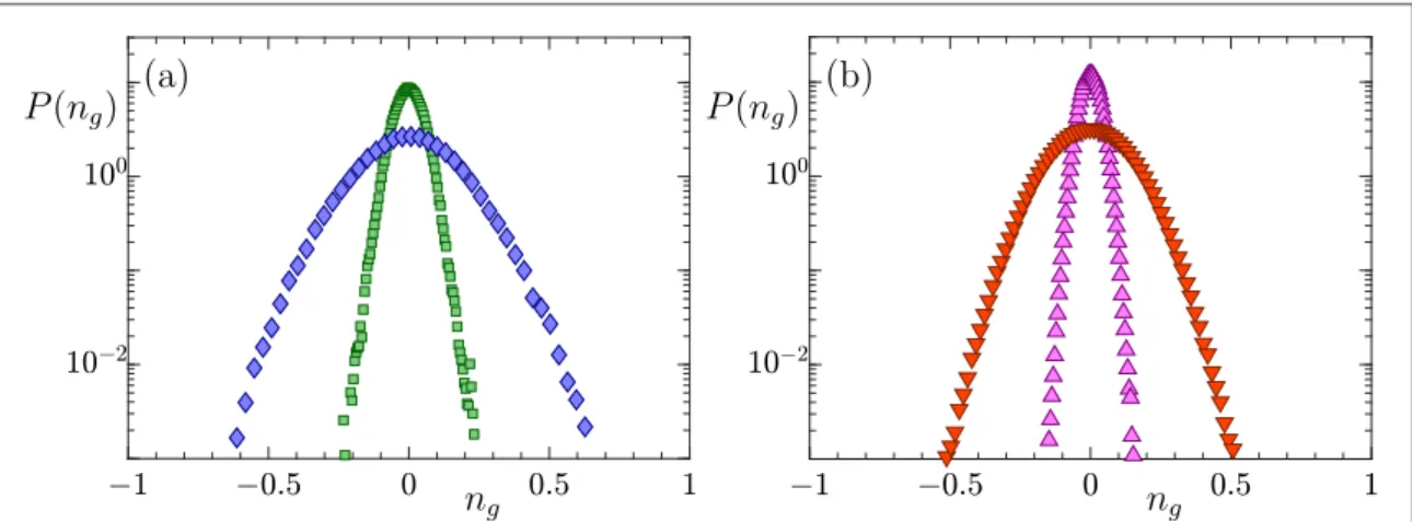
Figure2shows orientation distributions obtained by numerical simulations of equations(14) for the

three-dimensional statistical model described in section2.2. Shown are distributions ofng =n g· ˆfor rod-like particles with aspect ratioλ=5, for different Stokes and settling numbers. We see that the particles settle with their broadside approximately aligned with gravity, that is ng≈0. This is the stable orientation for prolate

particles settling in a quiescentfluid [25,26].

Compare the distributions infigure2to those shown in[48]. Figure1(b) of [48] corresponds to rods that

tend to settle tipfirst. The reason for the difference is that the effect of the fluid-inertia torque was neglected in [48], whereas in the present work we choose parameters where this torque dominates the angular dynamics.

When the Stokes number is small we expect that the vectorn spends most of its time close to a stable fixed point of the angular dynamics. As mentioned above, thisfixed point is ng=0 in the absence of turbulence. But

the turbulent velocity gradients must modify thisfixed point. How does this affect the orientations of the settling particles? Figure2shows that the orientation distribution is still peaked at ng=0, but that it acquires a finite

width. The question is how the width depends upon the parameters of the problem, on the settling number Sv and upon the Stokes number St. Figure2indicates that the width decreases as Sv increases atfixed St, and that the width increases as the Stokes number St increases atfixed Sv. In the following we first consider small Stokes numbers, because the problem simplifies in this overdamped limit. In this limit we expect that the particle orientation follows thefixed-point orientation quite closely. This allows us to derive a theory for the orientation distribution in this limit, described in the following section.

Figure 2. Distribution ofng =n g· ˆobtained by three-dimensional statistical-model simulations of equation(14) for rod-like particles with aspect ratio l = 5._{(a) Settling number}Sv=18, Stokes numbersSt=0.22_(green,) andSt=1.1_(blue,à_). (b)Sv=45,St=0.22(magenta,) andSt=2.2(red, ▿).

4. Overdamped limit

Assume that the relaxation time ofn is much faster than the time scale on which the gradients change as the particle moves through theflow. This corresponds to the overdamped limit of the problem,St0 in equations(14). It was shown by experiments and numerical simulations in [51] that this limit quantitatively

describes the orientation distribution of rods settling in a 2D vortexflow, and in the slender-body limit this approach was also used in[56,69].

We also assume that Sv is large enough so that thefluid-inertia torque dominates the angular dynamics. This allows us to take into account turbulentfluctuations perturbatively. It also means that we can approximate the instantaneous slip velocity by_W( )0( )_{n, equation(6). In this limit we find:}

= ( )( ) ( )

W W 0 n , 24a

A 

wp=W+ L(n n)+ Sv2ng(ngˆ), (24b)

withng =n g· ˆ, as defined in section3. The overdamped equation for the dynamics of the vectorn corresponding to equation(24b) reads

A

  

= + L - +

-˙ [ ( · ) ] ( ˆ ) ( )

n n n n n n Sv2ng g ngn. 24c

To simplify the notation we introduced the parameter

A=A¢ ^ ^ ^  ( ) I A A C . 25

Figure1(b) shows how A depends on the particle-aspect ratio λ.

4.1. Two-dimensional dynamics in the overdamped limit

We consider the 2D modelfirst because it is much easier to analyse than the three-dimensional model. We assume that the gravitational acceleration points into theeˆ1-direction, and define f to be the angle (  f0 <p)

betweenn and this axis, so thatng =n g· ˆ =cosf. For prolate particles(λ>1 or equivalently Λ>0) the overdamped angular dynamics(24c) becomes in two spatial dimensions:

A

f= -O + L[S cos 2( f)-S sin 2( f)]+ ∣ ∣Sv sin 2( f). (26)

t d d 12 12 11 1 2 2

This 2D overdamped equation of motion for the angular dynamics is essentially equivalent to model M2 in[51],

used there for simulations of the angular dynamics of rods settling in a 2D vortexflow. Apart from the fact that [51] considers a different flow, it describes small cylindrical particles with slightly different resistance tensors,

and it approximates then-dependence of the settling velocity. Equation (26) shows that the fluid-inertia torque

has the same angular dependence as the S11-component of the strain, but in general the sign may differ. When

S11>0, the strain tends to align the rod witheˆ1, the direction of gravity. Thefluid-inertia torque acts against

alignment with this direction. To quantify this statement, consider thefixed points of the angular dynamics (26).

In the limit A∣ ∣Sv2 ¥_{, the inertial torque dominates the angular dynamics, so that thefluid-velocity}

gradients do not matter. In this limit thefixed points are *f = 0₁ andf*₂ =p 2. For a prolate particle(λ>1) *

f = 0₁ is unstable whilef*₂ =p 2is stable. This is the limit considered in[25], a slender rod falling in a

quiescentfluid: sincef*₂is stable the rod settles with its broad sidefirst. The same is true more generally for prolate axisymmetric particles settling in a quiescentfluid [26].

Now, what is the effect of the turbulentflow? In general this question is difficult to answer. But if the angle f relaxes much faster than thefluid-velocity gradients change along the particle path, then the problem becomes tractable. Assuming that the gradients are constant, we canfind exact expressions for the two fixed points of equation(26), for arbitrary aspect ratios and fluid-velocity gradients. We take λ>1 and expand the stable fixed

point aroundπ/2 assuming that A∣ ∣Sv2_{is large:}

A A * f = p - - + ∣ ∣ ( ) ( ) B B B 2 1 Sv 2 1 Sv ... 27 2 12 2 11 12 2 2

Here Bijare the elements of the matrix =+ L . Equation (27) shows how the fixed-point orientation

*

f ( )₂ t changes as a function of ( )t , as the turbulent velocity gradients evolve. We expect that the orientation of a

settling rod follows thefixed-point orientation *f ( )₂ t quite closely in the overdamped limit, provided that its angular relaxation time is smaller than the time scale on which theflow (and thusf*₂) changes.

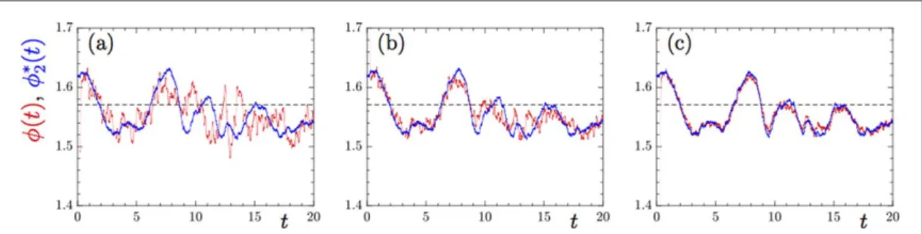
Figure3shows examples of how thefixed point *f ( )₂ t of the angular dynamicsfluctuates as the particle settles through the turbulentflow and encounters different fluid-velocity gradients. The data are obtained by numerical simulation of the 2D model described in section2, for small Stokes numbers. Also shown is the instantaneous angle f(t) obtained in these simulations. We see that the orientation dynamics follows the fixed pointf*₂quite closely when St is small. In this case the orientation distribution of the settling particle is determined by the distribution of

*

f₂, and thus by the distribution offluid-velocity gradients encountered by the particle, through equation (27). This

distribution may differ from the distribution offluid-velocity gradients at a fixed spatial position (preferential sampling[53]). But in the overdamped limit preferential sampling of the fluid-velocity gradients is expected to be

weak for settling particles. We have checked that it is negligible for data shown in this paper.

If we consider only the leading correction in equation(27), then the orientation distribution is determined

by the distribution PB(B12) of B12: A A

ò

(

)

In the 2D statistical model the distribution PB(B12) is Gaussian with variance s =B2 (2+ L)

1 8

2_{. This means that}

the distribution off is Gaussian too:

f ps = f -f p sf -( ) ( ) ( ) P e 2 , 29 2 2 2 2 2 with variance A s =_f + L (∣ ∣ ) ( ) 1 8 2 Sv . 30 2 2 2 2

Equation(28) shows that the distribution of f simply reflects the magnitude of the fluctuations of the

fluid-velocity gradients, at least when the particle orientation relaxes faster than thefluid-velocity gradients change (see below for a full discussion). The corresponding distribution ofng =n g· ˆis:

f f p s ps = = - -f f ( ) ( ) [ ( ( ) ) ( )] ( ) P n P n n 1 sin exp acos 2 2 2 1 . 31 g g g 2 2 2 2

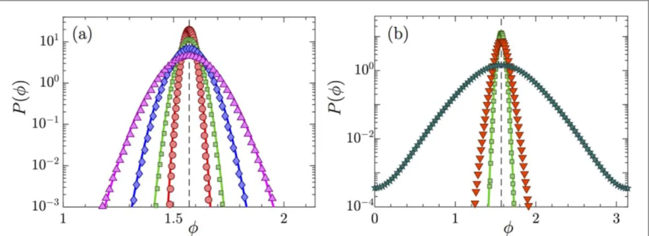
Figure4shows that equations(29) and (30) agree well with results of simulations of the overdamped dynamics in

two spatial dimensions, provided that St is small enough(panel (a)). In this case the orientation variance decreases asSv-4_{as Sv increases.}

The model predicts that the orientation distribution broadens as the particle aspect ratioλ increases (full lines). This is consistent with the numerical results (symbols), and can be readily explained by noticing that A∣ ∣ is a decreasing function ofλ, see figure1(b). As a consequence, the variance of the fluctuations,µ1 A2_,

increases asλ grows. When the Stokes number becomes larger [panel (b)], the distribution is much wider than predicted by the overdamped theory.

The theory outlined above assumes that the angular dynamics(26) responds so rapidly that the orientation

of the particle follows the instantaneousfixed point of the dynamical system (26) quite closely. To quantify more

precisely when this theory applies we must consider the relaxation timeτ_fof the angular dynamics. In units of

t_Kit is given by the inverse of the stability exponentσ of the fixed pointf*₂. In keeping with the assumptions underlying equation(27) we require

A 

∣ ∣Sv2 1. (32)

First, to leading order in A(∣ ∣Sv2)-1_{wefind from equation (26) thats ~ -∣ ∣SvA} 2_{. This gives}

A tf~∣s-∣= ∣ ∣ ( ) 1 Sv , 33 1 2

Figure 3. Angular dynamics of a settling particle in two spatial dimensions. Shown is the anglef( )t obtained by simulation of equation(14) (red), and the analytically exact result for the stable fixed pointf ( )*₂t (blue). (a)St=0.1,(b)St=0.05,(c)St=0.02. Other parameters: Sv_{=25, λ=5. The three simulations were performed with the same initial conditions and for the same realisation} of the function (u x t, )in the 2D statistical model.

and equation(32) implies that tf 1. Second, when Sv is large, thefluid-velocity gradients seen by the settling

particle change at the settling time scaleτs, the time it takes a particle settling with an anglef=π/2 at a settling

velocity given by equation(6) to fall one correlation length ℓ

t t t h = ℓA^ = ℓ ^ ( ) g A 1 Sv. 34 s K p K

We therefore conclude that the theory outlined above holds if

A t t h = f ^  ℓ ∣ ∣ ( ) A 1 Sv 1. 35 s K

This condition ensures that the gradient dynamics is‘persistent’ [70], in the sense that the fluid-velocity gradients

change much more slowly than the angular particle dynamics relaxes. Equation(35) indicates that the persistent

limit is achieved provided that A∣ ∣Sv is large enough, at least for the overdamped dynamics(26). For smaller

values of Sv the overdamped theory is modified in at least two ways. First, the fixed point (27) may annihilate in a

bifurcation withf*₁. Likewise, the time scaleτ_fmay depend on the instantaneousfluid-velocity gradients if the condition(32) does not hold. Second, the time scale at which the particle samples the fluid-velocity gradients is

different: at small Sv this time scale is no longerτs. Instead the Kolmogorov timeτKmust be used in

equation(35). Here we do not discuss this limit further. The results derived above, and in the remainder of this

paper, assume that the condition(32) is satisfied.

4.2. Three-dimensional dynamics in the overdamped limit

In this section we show how to obtain the distribution ofng =n g·^for the three-dimensional statistical model, in the same overdamped and persistent limit considered above. The calculation is analogous to the one described in section4.1. Let p=n-nggˆ. Usingp2 = -1 ng2we express the equation of motion(24c) of ngas

A A    = = + L - + -= + L - + - - + -˙ ˆ · ˙ ˆ · [ ˆ · ( · ) ] ( ) [( ) ( ) ] ( ) ( ) g n g n g n n n n n n n O n S n n S n S n n Sv 1 1 2 1 Sv 1 . 36 g g g g gp g gp g g gg g pp g g 2 2 2 2 2 2

Here the subscripts g and p denote contractions with ˆg andp. In the limit of A∣ ∣Sv2 ¥_{,n* =0}

g is the stable

fixed point for prolate particles (λ>1). To determine how the fixed point changes due to fluid-velocity fluctuations we seek an expansion in A_{(∣ ∣Sv}2₎-1_{as in section4.1, of the formn}* µ_{1 (∣A∣Sv)+ ¼}

g 2 . We obtain to leading order: A *= ˆ · ∣ ∣ ( ) g p n Sv . 37 g ₂

Assuming that the orientation ofpis uncorrelated from thefluid-velocity gradients, we obtain for the variance of the distribution of ng: A A s = á ñá∣ ∣ñ » s (∣ ∣ ) (∣ ∣ ) ( ) p B Sv Sv , 38 n2 12 B 2 2 2 2 2 2 2 g

wheres2Bis the variance of the distribution of B12(the gravitational acceleration points in theeˆ1-direction). We

also used thatp2 = -1 ng2»1. This is a good approximation because in the limit we consider ngis small for

prolate particles. Assuming thatpand thefluid-velocity gradients are uncorrelated implies that the distribution

Figure 4. Orientation distributions for the two-dimensional statistical model.(a) Distribution of angle f=acos(ng) obtained from numerical simulation of the dynamics(14) (markers) and the limiting theory for small Stokes numbers, equation (29) (solid lines).

Parameters:Sv=22,St=0.022, andλ=3 (red, ◦ ), λ=5 (green,), λ=7.5 (blue,à), λ=10 (magenta,). (b) Same, but for different Stokes numbers. Parameters:_{λ=5, and}St=0.022_(green,),St=0.22_{(red, ▿),}St=22_{(dark green, ).}

of ngis Gaussian in the statistical model: p s s = ⎛ -⎝ ⎜⎜ ⎞_⎠⎟⎟ ( ) ( ) P n 1 n 2 exp 2 , 39 g n g n 2 2 g g

and the variance evaluates to

A s = + L (∣ ∣ ) ( ) 1 Sv 5 3 60 . 40 n2 _{2 2} 2 g

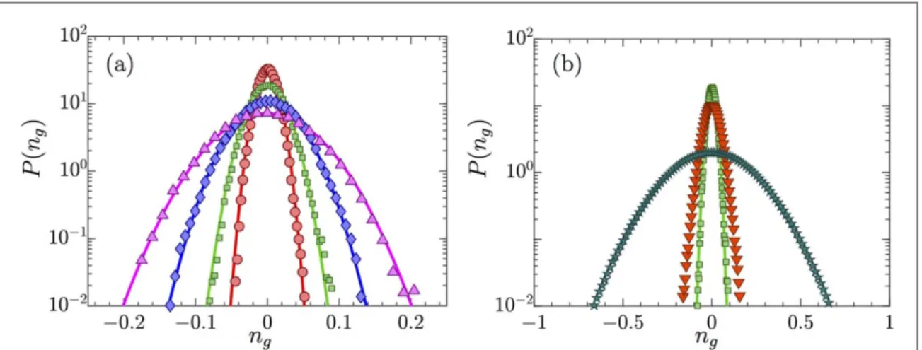
Figure5shows results for the distribution of ngfrom simulations of the three-dimensional statistical model.

Panel(a) shows results for small Stokes numbers, the parameters are the same as in figure4(a). Also shown are

the results of the theory, equations(39) and (40). In this case St is small enough and Sv large enough so that the

theory works very well. Panel(b) shows the orientation distribution for different Stokes numbers, to demonstrate how the theory fails when the Stokes number becomes larger. The behaviour is similar to that described in section4.1: the distribution widens as St increases.

Equation(38) says that the variance of the distribution of ngis inversely proportional to the fourth power of

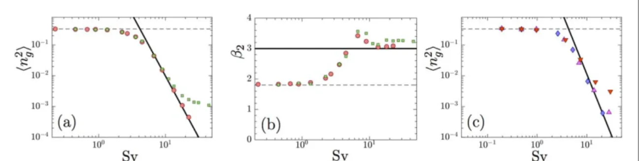
Sv, sn2g µSv-4, for large values of the settling number provided that the Stokes number is small enough. In figure6(a) this prediction is compared with results of simulations of the three-dimensional statistical model.

Shown is the variance of ngas a function of Sv, for two Stokes numbers. When the Stokes number is small we see

that the prediction(40) works well for large Sv, as expected. Figure6(b) shows the kurtosis b = á ñ á ñ2 ng4 ng2 2,

measuring theflatness of the distribution P(ng). As predicted by the theory, the kurtosis approaches the Gaussian

limit(β2=3) for large settling numbers, at small enough Stokes numbers.

WhenSv0 the variance tends to1

3and b 2 9

5, indicating that equation(40) fails because

condition(32) is no longer satisfied. In this limit the distribution of ngbecomes uniform and independent of the

Stokes number, because the angular dynamics is isotropic when gravitational settling is weak. Figure6(c) shows

results for the variance from numerical simulations using the KS model(section2.3), for three different values of

the Stokes number. The results are very similar to those obtained using the statistical model(figure6(a)). There is

good agreement with the overdamped theory, equation(38), at large Sv for small enough St. We determineds2_B

from the KS simulations, so there are nofitting parameters in figure6(c). The good agreement shows that the

overdamped theory is robust, insensitive to the details of the spectrum of the velocityfluctuations. Figure6also shows numerical data for larger values of St. For small Sv this makes little difference, the distribution is uniform. For larger Sv the numerical resultsfirst follow equation (38) or (40). But as Sv increases further, the overdamped

theory starts to fail, the earlier the larger the Stokes number. This indicates that particle inertia begins to become important.

The results obtained here rely on the statistical model described in section2.2, based on a simplified model

for the turbulentfluid velocity-gradients. In turbulence there are subtle correlations between vorticity and strain that are essential for the alignment between the rod direction and vorticity[30], in the absence of settling, and in

the overdamped limit. These correlations are neglected in the statistical model, but we argue that the results presented here are insensitive to these correlations. The alignment between orientation and vorticity builds up over a time scale of the order of a fewτK[71] (see also figure 1 of [30]). Since heavy settling particles do not follow

the motion offluid particles, the correlations between vorticity and strain do not play a significant role, in

Figure 5. Orientation distribution for the three-dimensional statistical model. Same conventions and parameters as infigure4.(a) ( )

particular for large Sv. This is consistent with comparisons between the results of DNS and of the statistical model in[48], showing quantitative agreement between the two approaches.

Finally we remark that the orientation distributions(29) and (39) are Gaussian in the statistical model. This

follows from the simplifying assumption that the velocity-gradient statistics is Gaussian. In turbulence this is not the case, as explained in section2.2. The overdamped theory shows that the angular distribution simply mirrors any non-Gaussian features of the turbulence velocity-gradient statistics, equation(28). Similarly, the relation

(38) between the orientation variance and the variances_B2_{holds also for turbulence—where the corresponding}

distributions are not Gaussian.

5. Beyond the overdamped limit

The overdamped theory in the previous section was derived for large Sv. Panels(a) and (c) of figure6show that this theory describes the numerical results very well. However, thefigure also exhibits deviations from the theory at very large values of Sv when the Stokes number is small, butfinite. To understand when and why the

overdamped theory fails one must check the full inertial dynamics. To this end we begin by analysing the 2D statistical model.

5.1. Two-dimensional model

To estimate the time scales that are important for the inertial angular dynamics, we consider the limit where the torque due tofluid inertia dominates over Jeffery’s torque, as in the previous section. In the overdamped limit this led to condition(32). For a qualitative analysis of the inertial angular dynamics we not only set the

fluid-velocity gradients to zero, = 0, but also thefluid velocity, =u 0. In this case the dynamics of the phase-space coordinatezº (vpx,vpy,f w, p)has the stablefixed point *z =(Sv A^, 0,p 2, 0 , where gravity points in the) direction ofeˆ1. The stability matrix follows from equation(14):

A A  º ¶ ¶ = -- -- ¢ + ¢ -^ ^ ^ ^ ^ ^ ^   ⎡ ⎣ ⎢ ⎢ ⎢ ⎢ ⎢ ⎢ ⎢ ⎤ ⎦ ⎥ ⎥ ⎥ ⎥ ⎥ ⎥ ⎥ ˙ ( ) z z A A A A A A A C I 1 St 0 0 0 0 Sv 0 0 0 0 St 0 Sv Sv , 41 2 2

whereA¢was defined in equation (17). The relaxation time following from equation (41) is given by

tf=max(-1 Rsi), the maximal stability time ofJ. HereRsidenotes the real part of the itheigenvalue of.

One eigenvalue of this matrix is s = -A^ St. We have computed the other eigenvalues numerically and

analytically in limiting cases. Wefind that the time scaletfinterpolates between equation(33) for small St and

~St A^for large St, for afixed value of Sv. If we fix St, by contrast, then we find that the time scale τf

interpolates between equation(33) for small Sv and ~St A^for large Sv. We remark, however, that if Sv is not

large enough, then one cannot justify to neglect thefluid-velocity gradients in the stability matrix (41), so that

any argument based on equation(41) must break down.

We expect that the overdamped approximation fails when the inertial estimate for the relaxation time of the angular dynamics, t ~f St A^, becomes larger than the overdamped estimate equation(33). This means that the

Figure 6. Width of the orientation distribution.(a) Variance of ngfrom simulations of the three-dimensional model, as a function of

Sv, for two values of the Stokes number:St=0.022(red, ◦) andSt=0.22(green,). Also shown is the theory for largeSv, equation(40), solid line, and the result for a uniform distribution,á ñ =ng2

1

3(dashed line). (b) Kurtosis b = á ñ á ñ2 ng ng 4 2 2_{. Same}

parameters as in panel(a). The overdamped theory (section4.2) gives a Gaussian distribution with kurtosis equal to β2=3 (solid line). For a uniform distribution,b =2

9

5(dashed line). (c) Results forsn 2

gfrom KS forSt=0.025(blue,à), 0.1 (magenta,), and 0.4

overdamped approximation requires

A  ^

∣ ∣Sv2 A St. (42) Conversely, when equation(42) is not satisfied then particle inertia matters, so that the overdamped

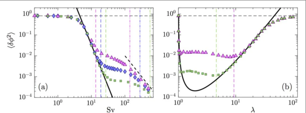
approximation must fail(figure6(a)). For a quantitative comparison, figure7(a) shows numerical results for the

variance of the orientation distribution obtained from simulations of the 2D model. We see that the overdamped approximation breaks down for values of Sv larger than~ A^ (∣A∣ )St , as predicted by equation(42). We observe that the variance decreases more slowly as Sv increases further.

Figure7(a) also reveals that there is yet another, asymptotic regime at very large values of Sv—so large that it

is difficult to achieve smallRepat the same time. It is nevertheless of interest to analyse this regime, because it

reveals the ingredients that a theory describing effects of particle inertia must contain. Figure7(a) suggests that

á ñ ~n c ( )

Sv 43

g2 1₂

for very large values of Sv. Our simulations indicate that the prefactor c1depends uponℓ hK, St, and uponλ

(not shown). We surmise that this regime describes particles settling so rapidly that the settling time scale τsis the

smallest time scale in the system. This cannot hold unless t ~f St A^is much larger thanτs, and this crossover

occurs at h ~ ^ ℓ ( ) A Sv St 1. 44 2 K

We expect equation(43) to be accurate for values of Sv much larger than those given by equation (44). This

condition is also shown infigure7, and we see that the large-Sv regime starts at values of Sv approximately satisfying(44). Since condition (42) is violated in this regime, particle inertia must be taken into account. A

difficulty is that particle inertia changes the translational as well as the angular dynamics. Thus it is no longer guaranteed that_W=_W( )0( )_{n (assumed in the overdamped theory of section4). This means that particle inertia} is expected to modify the angular dynamics in at least two ways. Firstly, it introduces the time derivative df

t

d d

2 2

into the angular dynamics. Secondly, thefluctuations of the torque change because_W¹_W( )0( )_{n when particle} inertia matters. This is discussed in section5.2.

Figure7(b) shows how the variance ofδfdepends on particle shape, for fixed Sv and St. There are four

regimes. First, in the limit l  ¥ the distribution is uniform and independent of the Stokes number. In this regime the dynamics is overdamped(condition (42)), but the persistent approximation fails because

equation(32) is not satisfied. Second, for intermediate aspect ratios, both conditions are satisfied, so that the

theory(equations (29) and (30)) is accurate. Third, as λbecomes smaller, the overdamped approximation

breaks down. In this regime particle inertia must be taken into account. Fourth, asλ→1 the orientation distribution must become uniform. This cross-over happens very rapidly: for spheres(λ=1) the orientation distribution is uniform, but already forλ∼1.05 there is strong alignment.

We conclude this section with a remark concerningfigure7(b): the overdamped theory (30) predicts that the

variance ofδf grows as the aspect ratio λ increases, provided that St and Sv are kept constant. In physical terms this is a consequence of the fact that the mobility coefficients become smaller as λ increases. A smaller

Figure 7. Variance dfá 2ñ_{for the two-dimensional statistical model.(a) Results of numerical simulations as a function ofSvfor l = 5,}

=

St 0.1(green,),St=0.2(blue,à),St=0.4,(magenta,). Also shown: theory from section4.1, equations(29) and (30), thick

solid black line; condition A∣ ∣Sv2=A^ St_{for the overdamped theory to fail[equation (42)], vertical dashed lines; condition (44) for} the white-noise limit, vertical dashed–dotted lines; large-Svscaling(43), thick black dashed line; uniform distribution at smallSv, horizontal black dashed line._{(b) Results as a function of the particle aspect ratio λ for}Sv=25,St=0.1_(green,), andSt=0.4 (magenta,).

translational mobility(A-1andA^-1) reduces the magnitude of the slip velocity in equation (14d), while smaller

rotational mobilityI C^ ^-1increases the effect of thefluid-velocity gradients upon the angular dynamics of the

particle. Both tendencies diminish the effect of thefluid-inertia torque in equation (14d) as λ grows, diminishing

its tendency to align the particles. This prediction is in good agreement with the 2D simulation results shown in figure7(b).

5.2. Klett’s small-angle expansion

Klett[28] proposed a theory for the orientation variance of nearly spherical particles settling in turbulence,

including particle inertia in the angular dynamics. He uses that the orientation variance is very small for large values of Sv. This suggests to expand the equations of motion in small deviations of the angle f =acos( · ˆ)n g

from its equilibrium value:f=f*+dfwhere *f = p

2for prolate particles. Klett assumes that = ( ) ( )

W W 0 n

(equation (6)) and expands the angular dynamics for nearly spherical particles in δf.

We can derive an equation of motion consistent with his by expanding equations(14) to leading order in δf,

assuming that_W=_W( )0( )_{n , retaining only the leading terms in A(∣ ∣Sv}2₎-1_{(we must also require that St is}

small, in keeping with Klett’s assumptions). In this way we obtain for a prolate particle of arbitrary aspect ratio in three spatial dimensions:

A  df+ ^ df+ df= -^ ^ ^ ^ ^ ∣ ∣ gˆ · p ( ) t C I t C I C I d d St d d St Sv St . 45 2 2 2

When we expand the geometrical coefficients in equation (45) for small Λ we find that the prefactors of the terms

on the lhs of this equation are almost identical, in this limit, to those in equation(17) of [28]. Slight discrepancies

arise in theδf-term because we use the expression for the inertial torque from [26], while Klett uses the form

obtained by Cox[24] (the relative error of the prefactors is of the order of 10−3[26]). At any rate, equation (45) is

simply a damped driven harmonic oscillator, with implicit solution



ò

HereW =0 [C^ (2 StI^ )] 4∣A∣Sv2I^St C^-1. Note that we discarded terms related to the initial angle, because they cannot be important for the steady-state variance ofdfin the limit of large Sv, atfixed St. Squaring equation(46) and averaging over realisations of the turbulent fluctuations in the statistical model we obtain for

large Sv df á ñ ~ c ( ) Sv , 47 2 0 4

where c0is a function ofℓ h_K, St, and of the aspect ratioλ. We neglected aSv-3contribution toádf2ñbecause it

is exponentially suppressed. Equation(47) fails to describe the large-Sv behaviour (43), shown as the thick black

dashed line infigure7. This means that equation(45) cannot be used to estimate the large-Sv width of the

orientation distribution, or to compute deviations from the overdamped theory.

Which approximation causes equation(45) to fail? Since the variance is small for large Sv,dfremains small at all times. Therefore we see no reason to doubt that the small-angle expansion is valid. This leads us to conclude that the assumption_W=_W( )0( )_{n breaks down, in agreement with our conclusions in the previous section. To} check this, we artificially imposed the constraint_W=_W( )0( )_{n in simulations of the 2D statistical model. The} resulting large-Sv variance follows equation(47), and thus fails to give the correct scaling, equation (43). This

demonstrates that it is important to allow W to deviate from_W( )0( )_{n when particle inertia matters.} Klett obtains that dfá 2ñ µ Sv-2_{, assuming that thefluid-velocity gradients on the right-hand side of}

equation(45) are just white noise in time. This scaling is consistent with the large-Sv power law observed in

Figure7(a), but Klett’s theory is difficult to justify from first principles because it neglects fluctuations of

- ( )( )

W W 0 nt _{that yield additional time-dependent terms in the angular equation of motion(45), which are}

expected to affect the prefactor of the Sv-2scaling. More importantly, the 2D simulation results shown in figure7demonstrate that dfá 2ñ µSv-2_{applies only in the unphysical limit of very large Sv, and that particle}

inertia causes a complex parameter dependence of the orientation variance at smaller values of Sv, with a number of different regimes to consider.

6. Conclusions

Convectivefluid inertia affects the orientation of a small axisymmetric particle settling in a turbulent flow. In [5,6,47–49] this effect was neglected. Here we considered a limit of the problem where it is dominant, but where

turbulentfluctuations still matter. This limit is relevant to computing the distribution of orientation of ice crystals settling in turbulent clouds[1]. Our goal was to compute the distribution of orientations of a spheroid in