HAL Id: hal-00866448
https://hal.archives-ouvertes.fr/hal-00866448
Preprint submitted on 30 Sep 2013
HAL is a multi-disciplinary open access
archive for the deposit and dissemination of sci-entific research documents, whether they are pub-lished or not. The documents may come from teaching and research institutions in France or abroad, or from public or private research centers.
L’archive ouverte pluridisciplinaire HAL, est destinée au dépôt et à la diffusion de documents scientifiques de niveau recherche, publiés ou non, émanant des établissements d’enseignement et de recherche français ou étrangers, des laboratoires publics ou privés.
Integrated Modelling of Economic-Energy-Environment
Scenarios - The Impact of China and India’s Economic
Growth on Energy Use and CO2 Emissions
Fabien Roques, Olivier Sassi, Céline Guivarch, Henri Waisman, Renaud
Crassous, Jean Charles Hourcade
To cite this version:
Fabien Roques, Olivier Sassi, Céline Guivarch, Henri Waisman, Renaud Crassous, et al.. Integrated Modelling of Economic-Energy-Environment Scenarios - The Impact of China and India’s Economic Growth on Energy Use and CO2 Emissions. 2009. �hal-00866448�
DOCUMENTS DE TRAVAIL / WORKING PAPERS
No 15-2009
Integrated Modelling of
Economic-Energy-Environment Scenarios,
The Impact of China and India’s Economic
Growth on Energy Use and CO2 Emissions
Fabien Roques
Olivier Sassi
Céline Guivarch
Henri Waisman
Renaud Crassous
Jean-Charles Hourcade
March 2009C.I.R.E.D.
Centre International de Recherches sur l'Environnement et le Développement
UMR8568CNRS/EHESS/ENPC/ENGREF /CIRAD /METEO FRANCE
45 bis, avenue de la Belle Gabrielle F-94736 Nogent sur Marne CEDEX
Abstract
A hybrid framework coupling the bottom-up energy sector WEM model with the top-down general equilibrium model IMACLIM-Ris implemented to
capture the macroeconomic feedbacks of Chinese and Indian economic growth on energy and emissions scenarios. The iterative coupling procedure captures the detailed representation of energy use and supply while ensuring the microeconomic and macroeconomic consistency of the different scenarios studied. The dual representation of the hybrid model facilitates the incorporation of energy sector expertise in internally consistent scenarios. The paper describes how the hybrid model was used to assess the effect of uncertainty on economic growth in China and India in the energy and emissions scenarios of the International Energy Agency.
Keywords : hybrid modelling, general equilibrium model, energy demand
scenarios.
Résumé
Une structure hybride couplant le modèle WEM ‘bottom-up’ du secteur énergétique avec le modèle IMACLIM-R ‘top-down’ d’équilibre général est
appliquée pour saisir les rétroactions macroéconomiques de la croissance économique indienne et chinoise sur les scénarios énergétiques et d’émissions. La procédure itérative de couplage restitue la représentation détaillée des usages et de l’offre énergétiques en assurant la cohérence micro- et macro-économique des différents scénarios étudiés. La représentation duale du modèle hybride facilite l’incorporation de l’expertise du secteur énergétique dans des scénarios cohérents sur le plan interne. Ce document décrit l’utilisation faite du modèle hybride pour évaluer l’effet de l’incertitude sur la croissance économique en Chine et en Inde dans les scénarios énergétiques et d’émissions de l’Agence Internationale de l’Energie.
Mots-clés : modèle hybride, modèle d’équilibre général, scénarios de
Integrated Modelling of Economic-Energy-Environment
Scenarios - The Impact of China and India’s Economic Growth on
Energy Use and CO2 Emissions
Fabien Roques*, Olivier Sassi#, Céline Guivarch#, Henri Waisman#, Renaud Crassous#, Jean-Charles Hourcade#
*EPRG, University of Cambridge #
Centre International de Recherche sur l’Environnement et le Développement (CIRED) 16 November 2008
1 INTRODUCTION
The twin challenges of energy security and climate change have driven an intense modelling activity of long term energy-economy-environment (E3) scenarios over the past decade. As a global policy consensus on the reality of climate change and on the urgency to act is emerging, policy makers are increasingly looking for advice on short- to medium-term policies consistent with the longer-term objective of climate change and energy security threats mitigation. In parallel, knowledge about the various technological, economic and social dimensions of climate change is building up, such that the integration of these different dimensions in a consistent modelling framework is more challenging than ever. This joint dynamic is defining a new challenge for the modelling community in the years to come, calling for integrated cross-disciplinary modelling frameworks with a focus on high resolution short- to medium-term realistic trajectories and actions within longer-term consistent scenarios.
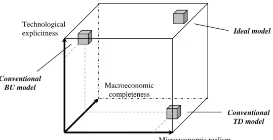
Models used in the economy-energy-environment research community have traditionally been categorised as either “top-down” (TD) models or “bottom-up” (BU) models. The so-called “bottom-up” models describe in detail current and future energy technologies on the demand and supply side, but lack a realistic portrayal of microeconomic decision-making by businesses and consumers when selecting technologies, and fail to represent potential macroeconomic feedbacks. They also lack an integrated macroeconomic framework to evaluate different energy pathways and policies in terms of changes in welfare, productivity and trade. In contrast, the so-called “top-down” models address these deficiencies by representing macroeconomic feedbacks in a general equilibrium framework; but their aggregate representation of the energy sector lacks a realistic description of the corresponding technologies and regulations that drive its evolution. Hourcade et al. (2006) provide a synthesis of the BU/TD division and a graphical representation of the three dimensions differentiating BU and TD models1 (Figure 1).
Technological
explicitness Ideal model
Microeconomic realism Macroeconomic completeness Conventional TD model Conventional BU model
Figure 1 : Representation of BU and TD models’ strengths and weaknesses. Source: Hourcade et al. (2006)
This traditional dichotomy has been gradually phased out over the past decade and much research effort have been concentrated on the development of “hybrid” models benefiting from the advantages of bottom-up and top-down models (Boringher, 1998; Hourcade et al., 2006). Such “hybrid” frameworks combine to various degrees technological explicitness, microeconomic realism and macroeconomic feedbacks. The hybridisation process can take different forms. Some original bottom-up or top-down models can evolve toward a hybridised architecture. This often means that BU models include macro-economic feedbacks (Manne and Wene, 1992) or micro-economic realism (Rivers and Jaccard, 2005) for technology choices in their architecture or TD models incorporate explicit technology description in their general equilibrium framework (McFarland et al., 2004)2. Another approach consists in coupling two existing BU and TD models. Despite some computational obstacles and some problems emerging from the inability of existing models to embark external data, such attempts3 have shown promising results and opened the path to a broader interaction between BU and TD analysis.
This is the strategy that has been chosen by the IEA to assess the macroeconomic effects of the uncertainty on the rate of economic growth in China and India in its 2007 E3 scenarios. In preparation to the 2007 edition of the World Energy Outlook, the IEA jointly developed with CIRED the WEM-ECO model – a hybrid model resulting from the coupling of the World Energy Model (WEM) and the IMACLIM-R model. The former is a technology-rich partial equilibrium model of the energy sector, developed at the IEA, updated annually to compute the World Energy Outlook global energy scenarios up to 2030. The latter is a recursive
2
Even if the MARKAL-MACRO model developed by Manne and Wene (1992) resulted in the coupling of a large BU model with a macro module, the previous examples mainly refer to modifications of existing architecture toward hybridisation.
3
For example, Drouet et al. (2004) produced a coupled model between a computable general equilibrium model of the Swiss economy and a MARKAL model of the Swiss housing sector. At a wider scale, Schafer and Jacoby (2005) informed the transportation sector of the EPPA world general equilibrium model through a coupling with a MARKAL model and a modal split model.
general equilibrium model developed at CIRED and built as a tool for incorporating data from external expertise or bottom-up models.
The contribution of this paper is twofold: first it brings a detailed description of the WEM-ECO coupling methodology, second it aims to illustrate how such a modelling architecture was used in the particular context of the IEA to capture the knowledge embodied in the organisation’s experts around a unique tool for dialogue. WEM-ECO was used to determine how the economy and energy consumption in each region of the world may be affected by higher GDP growth assumptions in China and India as compared to the baseline. Higher growth in China and India is likely to affect the economies of the rest of the world mostly through its impact on international commodity prices and on overall trade in all types of goods and services. The higher GDP growth rates assumed in such High Growth Scenario result in faster growth of energy demand in both countries, which leads to higher energy prices, that in turn reduce energy demand in energy importing countries. As for global trade and growth, we found that the impacts are not straightforward as they are influenced by general equilibrium effects, channelled through commodity prices and trade retroactions.
The next section describes successively the architecture of the hybrid model WEM-ECO and its source models WEM and IMACLIM-R, emphasizing the rationale of each architecture. The third section describes the coupling procedure and the different levels of integration of the two models that are possible. It also analyses the benefits of the WEM-ECO modelling framework to incorporate the expert judgment embodied in an organisation like the IEA. The final section illustrates the use of the WEM-ECO model to study the macroeconomic impact of a higher economic growth rate in China and India than in the baseline scenario.
2 THE HYBRID MODELLING FRAMEWORK WEM-ECO
2.1 The model WEM-ECO
As a partial equilibrium model of the world energy sector, the International Energy Agency WEM model guaranties a very detailed representation of the specific mechanisms that drive energy trends and especially those resulting from technological changes. Nevertheless the overall dynamic of the model rests on exogenous assumptions on population and on the growth and structure of GDP, that determine the evolution of various activity variables. These activity variables are used to compute the demand for specific energy services, the production of which requires the consumption of final energy depending on the technical characteristics of related energy equipment. Although a price elasticity is often used to represent the feedback of price variation on the formation of energy demand, the general consistency between (i) macroeconomic assumptions (growth and structure of the GDP) (ii) changes in energy prices and (iii) the evolution of technological characteristics of the energy sector is not guaranteed by such a framework.
On the other hand, IMACLIM-R, as a general equilibrium model, generates economic trajectories which present a strong internal consistency between economic and energy trends. Nevertheless the detail of the energy sector remains poor, especially for technological parameters. The willingness to build a modelling framework resulting from the coupling of two pre-existing models rests on the recognition that both approaches are complementary, so that the hybrid model resulting from the coupled architecture can gather the advantages from the two pre-existing models.
The WEM-ECO hybrid model has been specially designed to ensure a strong macroeconomic consistency of energy and environment scenarios and to facilitate the debate on key drivers and parameters. A key concern was to break the so-called “black box” syndrome that undermines interaction with the sectoral and technological experts. The two modelling priorities were therefore: (i) to construct an integrated hybrid model whose structure would facilitate the incorporation of expert judgment from the IEA’s specialists and the energy community; and (ii) to offer a modular and flexible architecture which would make possible to adapt the depth of analysis to the policy question to be addressed by the modelling exercise through a choice between an aggregated and a fully-integrated version of the model.
The hybrid WEM-ECO model feeds the output of the well-calibrated energy sector model WEM as an input into the well-calibrated general equilibrium model IMACLIM-R (Figure 2). In turn some of the calibration assumptions of the WEM model are modified based on the outputs of the IMACLIM-R model. This iterative process is stopped once the two models converge on an internally consistent set of macroeconomic and energy sector parameters. Section 3 details the coupling procedure and the different levels of integration of the two models that can be achieved. The next two subsections introduce successively the structure of the WEM and IMACLIM-R models.
Technology rich Bottom up Model WEM Hybrid Model WEM-ECO Macroeconomic top down Model
IMACLIM-R
Dialog with policy makers
Figure 2 : The WEM-ECO model as an integrator of different expertise
2.2 The IEA World Energy Model (WEM)
The World Energy Model (WEM) has been developed internally to the IEA since 1993 and is now in its 10th version. Most of the data are obtained from the IEA’s own databases of energy and economic statistics, and are complemented from a wide range of external sources.
WEM is an energy sector partial equilibrium model which provides short- to medium-run energy demand and supply projections. It is made of 21 regional or country blocks (c.f. Appendix 1). Contrary to optimisation models (like MARKAL type models), the WEM model is a simulation model with a yearly step and based on a modular structure. This architecture
choice is grounded in the short- to medium-term time horizon (2030), and reflects the willingness to have a modelling tool facilitating the interaction with the many experts of the IEA through multiple run iterations, and taking advantage of the rich IEA databases. The WEM is made up of six main modules: final energy demand, power generation, refinery and other transformation, fossil fuel supply, CO2 emissions, and investment. Figure 3 provides a simplified overview of the model’s structure.
The main exogenous assumptions concern economic growth, demographics, international fossil fuel prices and technological developments. Electricity consumption and electricity prices dynamically link the final energy demand and power generation modules. The refinery model projects throughput and capacity requirements based on global oil demand. Primary demand for fossil fuels serves as input for the supply modules. Complete energy balances are compiled at a regional level and the CO2 emissions and energy-supply investment are then
calculated using carbon factors.
Economic growth assumptions for the short- to medium-term are based on those prepared by the Organisation for Economic Co-operation and Development, the International Monetary Fund and the World Bank. Over the long-term, growth in each region is assumed to converge to an annual long-term rate, which depends on demographics, macroeconomic conditions and the pace of technological change. Rates of population growth for each region are based on projections from the United Nations (2004). And as a prominent scenario driver, average retail prices of each fuel used in final uses, power generation and other transformation sectors are derived from assumptions about the international prices of fossil fuels. The detailed structure of the model is presented in Appendix 1.
Figure 3 : World Energy Model Overview
2.3 The IMACLIM-R model
IMACLIM-Ris a hybrid recursive general equilibrium model of the world economy divided into
12 regions and 12 sectors (Sassi et al., 2007) and solved in a yearly time step. The base year of the model (2001) is built on the GTAP-6 database that provides, for the year 2001, a balanced Social Accounting Matrix (SAM) of the world economy The original GTAP-6 dataset has been modified (i) to aggregate regions and sectors according to the IMACLIM-Rmapping (see
As a general equilibrium model, IMACLIM-R provides a consistent macroeconomic framework to assess the energy-economy relationship through the clearing of commodities markets. Specific efforts have been made to build a modelling architecture allowing easy incorporation of technological information coming from bottom-up models and experts’ judgement within the simulated economic trajectories. Incorporating rigorously such information about how final demand and technical systems are transformed by economic incentives is made possible in IMACLIM-R thanks to the existence of physical variables characterizing explicitly equipments and technologies (e.g. cars’ efficiency, intensity of the production in transport). The economy is then described both in money metric values and in physical quantities linked by a price vector. This dual vision of the economy is a precondition to guarantee that the projected economy is supported by a realistic technical background and, conversely, that any projected technical system corresponds to realistic economic flows and consistent sets of relative prices.
The full potential of the dual representation of the economy in both financial and physical terms that characterises IMACLIM-R could not be exploited without abandoning the use of conventional aggregate production functions. After Berndt and Wood (1975) and Jorgenson (1981), those functions were admitted to mimic the set of available techniques and the technical constraints impinging on an economy. But regardless of the issue of their empirical robustness4, and whatever their mathematical form, they are calibrated on cost-shares data of the calibration year through the Shepard's lemma. The domain within which this systematic use of the envelope theorem provides a robust approximation of real technical sets is limited by (i) the assumption that economic data, at each point in time, result from an optimal response to the current price vector and (ii) the lack of technical realism of constant elasticities over the entire space of relative prices, production levels and time horizons under examination in sustainability issues.
IMACLIM-R is thus based on the recognition that it is almost impossible to find functions with mathematical properties suited to cover large departures from the reference equilibrium and flexible enough to encompass different scenarios of structural change resulting from the interplay between consumption styles, technologies and localisation patterns (Hourcade, 1993). The absence of a formal production function is compensated by a recursive structure (Figure 4) that allows a systematic exchange of information between:
• An annual static equilibrium module, in which the production function mimics the Leontief specification, with fixed equipment stocks and intensity of intermediary inputs (especially labour and energy), but with a flexible utilisation rate. Solving this equilibrium at t provides a snapshot of the economy at this date: a set of information about relative prices, levels of output, physical flows and profitability rates for each sector and allocation of investments among sectors;
• Dynamic modules, including demography, capital dynamics and sector-specific reduced forms of technology-rich models which take into account the economic values of the previous static equilibria, assess the reaction of technical systems. This information is then sent back to the static module in the form of new input-output coefficients to calculate the equilibrium at t+1.
4 Having assessed one thousand econometric works on the capital-energy substitution, Frondel and Schmidt conclude that “inferences obtained from previous empirical analyses appear to be largely an artefact
of cost shares and have little to do with statistical inference about technology relationship” (Frondel
Between two equilibria, technical choices are fully flexible for new capital only; the input-output coefficients and labour productivity are modified at the margin, because of fixed techniques embodied in existing equipment and resulting from past technical choices. This general clay putty assumption is critical to represent the inertia in technical systems and the role of volatility in economic signals.5
Technically, the IMACLIM-R model generates an economic trajectory by solving successive
yearly static equilibria of the economy interlinked by dynamic modules. Within the static equilibrium, in each region, the demand for each good comes from household consumption, government consumption, investment and intermediate uses from other production sectors. This demand can be provided either by domestic production or imports and all goods and services are traded on world markets. Domestic and international markets for all goods – not including factors such as capital and labour – are cleared by a unique set of relative prices that depend on the behaviours of representative agents on the demand and supply sides. The calculation of this equilibrium determines the following variables: relative prices, wages, labour, quantities of goods and services, value flows.
by a unique set of relative prices that depend on the behaviours of representative agents on the demand and supply sides. The calculation of this equilibrium determines the following variables: relative prices, wages, labour, quantities of goods and services, value flows.
Moving the Envelope of Technical Possibilities: Reduced Forms of Technology-rich Models
t
- New Equipment stocks - New Technical Coefficients - Relative prices - Savings - Investment allocation Economic System Technical Constraints
Annual Consistent Static Macroeconomic ‘Snapshot’
t
Figure 4 : Iterative Top-down / Bottom-Up dialogue in IMACLIM-R
3 IMPROVING THE CONSISTENCY OF ENERGY SCENARIOS USING THE WEM-ECO HYBRID
3 IMPROVING THE CONSISTENCY OF ENERGY SCENARIOS USING THE WEM-ECO HYBRID FRAMEWORK
When integrating a bottom-up and a top-down model, the most important issue lies in the intrinsic capability of one model to easily embark information coming from the other one and more fundamentally to share overlapping modelling areas where dialogue between the two models is possible. This issue is particularly problematic when coupling a CGE model with a partial equilibrium model of the energy sector. Indeed, most general equilibrium models use pre-determined production functions to represent the sectors’ set of available producing techniques. The information provided by the BU model is used to produce a better calibration of these functions. As an example, Schaffer and Jacoby (2005) used a BU model of the transportation sector to improve the calibration of the elasticity of substitution and autonomous energy efficiency gains that parameterise transportation energy consumption
5 In this version of the model, early scrapping of capita and retrofit are not represented. This limitation will be solved
within the EPPA model. This work can hardly be reproduced at a more generalised level because of the constraints resulting from the mathematically predetermined form of the production functions that are used in such a model.
The specific structure of the IMACLIM-R model simplifies the coupling procedure with a partial equilibrium model. First the IMACLIM-R structure gathers a general equilibrium framework and a detailed description of the energy sector for final demand, transformation and primary supply. Energy flows are expressed in physical terms and energy commodities are not traded under Armington assumption, which makes possible (i) to maintain physical energy conservation when importing or exporting and; (ii) to have better exogenous control on energy trade flows in order to take on board information from WEM model runs.
Second, each part of the energy sector in the IMACLIM-R model is associated with regional productive capacity, the evolution of which can easily be controlled on a yearly step and linked with the corresponding investment requirements. These productive capacities find their exact correspondences in the WEM model and thus are ideal coupling variables. Similarly, the production of energy services for final consumption for households or productive sectors is not represented through any predetermined production function (and the same is true for the transformation process of primary into final energy). The production technology is instead modelled through the use of input output coefficients, the evolution of which is controlled in the dynamic module on a yearly basis. These technical coefficients can therefore be iteratively modified during the coupling procedure to adjust to the amount of energy consumption generated by the WEM model, thereby revealing the technical evolution underlying the WEM model energy trend.
3.1 Coupling variables in the two models
The WEM-ECO model, resulting from the coupling of WEM and IMACLIM-R, is built on an
iterative exchange of information between the two models (Figure 5).
From an analytical point of view, running WEM requires a set of assumptions on technological parameters and exogenous economic drivers which can be divided into three subsets:
• A set of assumptions on activity variables, noted {AV} ; • A set of assumptions on energy prices, noted {PE} ;
• A set of parameters driving the various sectoral modules, noted {ps}.
In turn, the set of assumptions that are required to run the IMACLIM-R can be divided into three
subsets:
• A set of assumptions regarding technical coefficients’ evolution for the energy sector, noted {TCE};
• A set of assumptions on the exogenous evolution of non energy drivers (e.g. population, labour productivity…), noted {MC} ;
• A set of parameters driving non energy sectoral modules, noted {pmnes}.
The coupling procedure consists of an iterative modification of the drivers of each model using the information coming from the other. For WEM, the assumptions gathered in the subsets {AV} and {PE} can be modified by the coupling process, while those from {ps} remain fully exogenous. In the IMACLIM-R model, {TCE} can be modified by the coupling
process, while {MC} and {pmnes} remain fully exogenous. A scenario is considered harmonised when this iterative procedure converges to a stationary solution in which energy related technical reactions from WEM no longer modify the activity variable and prices trends generated by IMACLIM-R and used as exogenous drivers in WEM.
Growth engine, Sector dynamics
Updated parameters (i-o coefficients, stocks, etc.)
Price-signals, Physical flows, Rates of return, Available investment
Static equilibrium t Static equilibrium t+1
Time Energy S u pp ly Energy D e man d L a b o r pro d uc ti v ity WEM
Figure 5: The recursive dynamic framework of WEM-ECO
3.2 The two coupling techniques
The “natural” way to exchange information between a BU and TD model would see the TD model providing activity variables and energy prices to the BU model, which would in return inform the TD model on the technical reaction of the energy sector. Nevertheless, in the specific IEA context, the benefits resulting from a greater degree of integration of the two models have to be balanced against the time devoted to this hybridisation procedure. A full integration of the two models is more demanding in computational and human resources and would have significantly slowed down the iterative process of simulations. We thus developed two coupling procedures:
• The first procedure is intended to draw some information at an aggregated level from the coupling exercise. The exchange of information between WEM and IMACLIM-R
takes place at the level of energy consumption and does not concern technical coefficients. Although it results in a partial harmonization of the two models, this first procedure converges more quickly to a stationary solution and requires less computational resources.
• The second procedure is more straightforward and rests on a more classical dialog between the two models, IMACLIM-R producing activity variables and energy prices, and WEM generating the technical reaction of the energy sector.
Both coupling procedures start with the choice of values for the subset of parameters that will not be modified during the coupling process. As the default parameterisation of the IMACLIM -R model is not fine-tuned for the short- and medium-run, macro assumptions from the WEM Reference Scenario6 are used to calibrate the growth drivers in the IMACLIM-R model (i.e. changes in labour productivity and active population). This calibration determines a potential growth in IMACLIM-R, while effective growth will eventually be endogenous and considered as a result of the coupling process. The parameterisation of the IMACLIM-R model is also modified to reflect expert views on macroeconomic patterns that underpin the basic WEM parameters and the Reference Scenario storyline. These assumptions mainly concern the future pattern of globalisation, market openness and the evolution of capital flows associated with the evolution of the current major macroeconomic disequilibria. For WEO 2007, the parameterisation of international trade elasticities was set in order to reflect a pursuit and increase of the globalisation process. As regard to capital flows that compensate trade imbalance in the base year of the model, it is assumed that imbalances tend to zero over the long run, reflecting the belief that these imbalances cannot last indefinitely and some mechanisms will appear to counterbalance current driving forces.
3.2.1 The aggregated coupling procedure
The first coupling procedure, that we may call the ‘aggregated coupling procedure’, consists in an exchange of time series, and not only an exchange of ex ante parameters of the models. IMACLIM-R receives from WEM a sequence of annual detailed energy balances that are used to iteratively force the corresponding technical coefficients in IMACLIM-R. The detail of the procedure can be structured as follows:
1. Run WEM with default values for {AV0}, {PE0} and {ps0} and get results for energy
flows for the whole energy sector (final demand, transformation and supply). 2. Proceed to iterative runs of the IMACLIM-R model, beginning with the calibrated values
for {pmnes0} and {MC0} and adjusting the values of {TCE} along the whole trajectory
to produce a scenario in which the energy flows (accounted in real physical quantities) match the corresponding WEM values. This process eventually produces a new set of sectoral activity variables {AV1} and energy prices {PE1}
3. Run WEM with new values for sectoral activity variables and energy prices {AV1},
{PE1}. Get results for energy flows for the whole energy sector.
4. Repeat stages 3. and 4. and stop using the criterion defined by Eq. 1 and 2
{
} {
}
(
k 1 k)
Max AV+ − AV <ε (1)
6 The World Energy Outlook Reference Scenario assumes that there are no new energy-policy interventions by
governments as off mid-2007. This scenario is intended to provide a baseline vision of how global energy markets are likely to evolve if governments do nothing more to affect underlying trends in energy demand and supply, thereby allowing alternative assumptions about future government policies to be tested (IEA, 2007).
{
} {
}
(
k 1 k)
Max PE + − PE <ε (2) When the process reaches its stationary solution, there is a complete similarity between the energy flows represented in WEM and the IMACLIM-R model: A run of WEM using the
activity variables and energy prices produced by IMACLIM-R gives energy balances that are
similar to those produced by the IMACLIM-R model. 3.2.1.1 The fully-integrated coupling procedure
The second coupling procedure, which can be referred to as the ‘fully-integrated coupling procedure’, is designed to achieve a deeper integration of the two models. It rests on the exchange of complete sets of technical coefficient and activity variable between the two models thus leading to a harmonisation of scenarios at a more accurate level of coupling. Keeping the same notations as previously, the coupling procedure becomes:
1. Run WEM with default values for {AV0}, {PE0} and {ps0} and get results for sectoral
energy technical coefficients {TCE0} and energy flows for the whole energy sector
(final demand, transformation and supply).
2. Run the IMACLIM-R model with the calibrated values for {pmnes0} and {MC0}, and
constraint the evolution of {TCE} to {TCE0}. This produces a new set of sectoral
activity variables {AV1} and energy prices {PE1}.
3. Run WEM with new values for sectoral activities variables and energy prices {AV1},
{PE1}. Get results for sectoral energy technical coefficients {TCE1}.
4. Repeat stage 2. and 3. and stop using the criterion defined by Eq. 1 and 2. Only the first, or aggregated, coupling procedure was used for the work that will be presented in the next sections of this paper. Therefore, in the following we refer to the first procedure when mentioning “coupling technique”, except when specified differently.
3.3 Facilitating dialogue with experts and conceptualising judgement in energy scenarios
Some of the modelling choices that led to the development of the hybrid WEM-ECO model need to be understood in the specific context of developing a set of internally consistent economy-energy-environment scenarios, which involves inputs from different communities of experts and modellers. The development of the WEM-ECO model proved to be a useful common framework to integrate inputs from both macroeconomists and energy sector experts; the WEM-ECO architecture with its dual representation of financial and energy flows facilitated the dialogue of the two communities of experts. The WEM-ECO model appeared in the context of the development of the International Energy Agency World Energy Outlook 2007 scenarios as a common unified tool for dialogue between macroeconomists and energy experts and in this way helped to capture the knowledge embodied in the different organisations involved.
The unified and common WEM-ECO modelling framework can facilitate dialogue between different communities of experts. Indeed, any sectoral expert has in mind an implicit specific vision of the future state of the word. Incorporating expert judgment to improve an energy
scenario is possible only if the expert and the scenario designer share the same implicit vision about the future economic context. For instance, the detailed description of the energy sector in the WEM model does not provide any detailed representation on the general macroeconomic context in which the energy scenario is incorporated. This context is either materialised through the choice of assumptions (on economic or demographic growth for example) or through the level of energy prices that reveal the underlying views on the level of tension on energy markets. Thanks to the comprehensive description of the whole economic system it provides, the WEM-ECO model can therefore be used to explicit some underlying assumptions driving the energy scenario. For instance, WEM-ECO can provide information on the structure of international trade and households’ consumption, which constitute valuable information to check the internal consistency of the economic-energy-environment scenario.
4 CONSISTENT ECONOMIC-ENERGY-ENVIRONMENT SCENARIOS: THE IMPACT OF CHINA AND INDIA’S ECONOMIC GROWTH ON ENERGY USE AND CO2EMISSIONS
The WEM-ECO model was used to generate the Reference and High Growth scenarios (HGS) of the World Energy Outlook 2007. The High Growth Scenario is built as a variant of the central Reference Scenario (RS) to test the impact on the world economy of a faster economic growth in China and India (IEA, 2007). The former is based on the assumption that GDP growth in China and India is on average 1.5 percentage points per year higher than in the later. This results in an average growth rate to 2030 of 7.5% for China and 7.8% for India. This section describes how the hybrid model WEM-ECO was used to define an internally consistent macroeconomic-energy-environment scenario in the High Growth Scenario..
4.1 Increasing pressure on energy supply
0.00 0.02 0.04 0.06 0.08 0.10 0.12 0.14 0.16 0.18 0.20
2005 2030 - Reference Scenario 2030 - High Growth Scenario
China India OECD
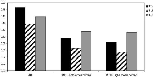
Figure 6 : Comparison of the GDP energy intensity in Reference and High Growth Scenarios, for selected regions
A first-order effect of additional economic growth in China and India is an increase in their demand for primary energy, which is 17.4% higher than in the Reference Scenario in 2030 (+1081 Mtoe). Yet the additional economic growth in China and India comes with a further
decoupling between energy and GDP, since the energy intensity in 2030 is respectively 12.5% and 16.7% lower than in the Reference Scenario (Figure 6). This decoupling results from the additional energy efficiency gains induced by higher energy prices and faster capital turnover, and a faster structural change.
Taking into account all macroeconomic feedbacks, the demand for primary energy worldwide increases by 6% in 2030, and global energy-related CO2 emissions are 7% higher in 2030 than in the RS at 44.8 Gt. The impact on energy demand differs across regions and depends on the GDP variations (which we will detail in the next section) and on the price sensitivity of demand. Demand increases in some regions and falls in others. The Middle East region sees the biggest increases in demand, increasing by 11% compared to the RS in 2030, because of its faster economic growth resulting from higher oil and gas prices. Conversely, energy demand in all three OECD regions, other developing Asian countries and Latin America falls slightly because of higher fossil fuel prices and lower economic growth than in the RS.
The additional energy demand from China and India is therefore the main driver of increased tensions in energy markets. The coupling procedure results in an increase in fossil fuel prices (Table 1) as the higher energy demand drives the exploitation of more expensive resources, while the investments in new production capacities by coal, oil and gas producers only partially adjust to the changing context.
2006 2010 2015 2020 2030
Oil price 0% 9% 17% 21% 40%
Natural gas price 0% 9% 17% 21% 40%
Coal price 0% 3% 7% 11% 19%
Table 1: Relative fossil fuel prices increase in the High Growth scenario w.r.t. the Reference scenario
4.2 Worldwide macroeconomic impacts of a higher growth in China and India
Higher growth in China and India affects the economies of the rest of the world through different and intertwined channels – the impact of higher energy prices on households’ consumption and on production costs, the competitiveness effects and the real exchange rates adjustments – which can have conflicting effects.
First, we show that higher growth in China and India increases the tensions on commodities markets, due to higher energy and raw material demand combined with supply side constraints. This has a negative impact on energy- and commodity-importing countries and a positive impact for exporting ones (Table 2). This effect is dominant for the Middle-East region, which benefits from a 10.9% higher GDP in 2030 compared to the RS. This is also the driving factor of slightly higher growth in Latin America (1.4%, due to oil exports from Venezuela) and Africa (1.4% also, due to oil and gas exports from Nigeria, Libya, Algeria). Second, a higher growth in China and India, and to a lesser extent in oil exporting countries, implies a larger demand for exports from the rest of the world, which would foster growth in the rest of the world. In fact this latter effect may in turn be partly offset by the readjustment of flexible real exchange rates in China and India in order to increase their exports and compensate their import requirements (under the constraint of a fixed capital balance). This
would imply losses of competitiveness for the other regions. The net effect hinges on the relative shares of increasing exports and increasing domestic demand in the additional growth in China and India. The balance between these two drivers of growth is critical to assess the impact on international markets.
The overall impact of the international trade effects on each region depends on its precise mix of exports and imports and its positioning in international trade and value chain. The results show slightly lower mean annual growth rates in the US, Europe and OECD Pacific (between minus 0.02% and minus 0.10% between 2005 and 2030). The positive impact of a higher demand of China and India for imports of advanced technology equipments and high value added goods from those regions is more than offset by the additional losses of competitiveness for other manufactured goods and materials and, mostly, by the economic impact of higher energy prices.
The Rest of Asia faces a reduction of GDP because the nature of their exports closely matches those of their giant neighbours, which makes them particularly vulnerable to the increase in the intensity of trade competition. Brazil falls in an intermediate position as it does not directly compete with China and India for international goods trade and its dependency on oil is reduced thanks to the development of biofuels.
Average annual growth rate,
2005-2030
Difference from Reference Scenario Average annual growth
rate, 2005-2030 Level of GDP in 2030 OECD 2.1% -0.06% -1.4% North America 2.4% -0.02% -0.4% United States 2.3% -0.04% -1.0% Europe 1.9% -0.10% -2.4% Pacific 1.8% -0.07% -1.8% CIS 3.5% 0.03% 0.6% Developing countries 6.2% 1.06% 30.2% Developing Asia 6.9% 1.28% 37.3% China 7.5% 1.50% 45.2% India 7.8% 1.50% 45.1% Middle East 4.4% 0.41% 10.9% Africa 4.0% 0.05% 1.4% Latin America 3.3% 0.06% 1.4% Brazil 3.1% -0.00% -0.1% World 4.3% 0.61% 16.3%
Table 2: World Real GDP Growth in the High Growth Scenario (average annual growth rates, %)
These economic growth projections must be interpreted with care given the large uncertainties on the pattern of growth and underlying capital flows. Capital flows are currently very unbalanced between China and the rest of the world (mainly the USA) and one critical assumption in the WEM-ECO model is that this imbalance is progressively reduced, the capital account converging to zero in the long run for all the regions, together with commercial flows. This is a common assumption in our field (e.g. Edmonds et al., 2004, Paltsev et al., 2005), but it remains a critical assumption.
In the following subsections we analyse two critical channels in order to disentangle the mechanisms at play behind the observed GDP differences: first, the changes in households’ consumption, and second, the changes in regional competitiveness and international trade.
4.3 Households’ consumption
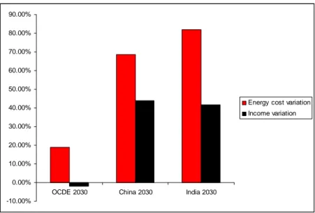
Higher energy prices in the High Growth Scenario largely increase the cost of providing energy services for households. Technical change induced by higher prices only partially offsets this increase, leading to higher energy spending in China, India and OECD in the High Growth Scenario (Figure 7). The pattern is nevertheless different for China and India compared to the OECD countries. Indeed, the latter experience a crowding out effect on the consumption of other goods and services as the total income decreases with reference to the Reference Scenario while the cost of energy spending increases. The situation is different in China and India where the share of energy expenditure over the total income increases with reference to the Reference Scenario, but the physical volume of household demand for non energy goods is still higher in the high growth scenario because of the higher income level.
-10.00% 0.00% 10.00% 20.00% 30.00% 40.00% 50.00% 60.00% 70.00% 80.00% 90.00%
OCDE 2030 China 2030 India 2030
Energy cost variation Income variation
Figure 7: Variation in real households’ income and energy spending in HGS w.r.t. RS
4.4 Regional competitiveness and international trade
4.4.1 Transmission of higher energy prices to production costs
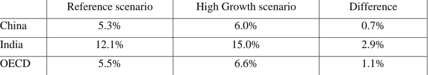
For goods- and services-producing sectors, the increase in energy prices increases production costs. The magnitude of this burden is related to the rate of turnover of equipments, and to the ability to finance early scraping of inefficient capacities. In the HG scenario, the share of energy costs in the total production costs of industrial good increases in all regions, but the magnitude of the increase differs on a regional basis (Table 3). China is relatively less impacted than India and OECD regions in the High Growth scenario, as its producing system mainly relies on coal as a primary energy source, whose costs increase relatively less than other primary fuels. OECD regions are more affected because their energy systems remain rather oil and gas intensive. India is even more affected because energy prices are linked to international prices whereas other costs (wages in particular) are linked to domestic prices,
and India experiences an important real exchange rate depreciation over the simulation period which gives an increased weight to energy prices.
Reference scenario High Growth scenario Difference
China 5.3% 6.0% 0.7%
India 12.1% 15.0% 2.9%
OECD 5.5% 6.6% 1.1%
Table 3: Shares of energy costs in total industrial production costs in 2030, in Reference and High Growth scenarios in China, India and OECD.
4.4.2 From production costs to competitiveness index: the role of real exchange rates
The energy burden weighing on production costs alters the profitability and competitiveness of production. The sectors with the highest inertia are particularly exposed to maladjustment and competitiveness losses. But real exchange rates play also a major role in modifying the different regions’ competitiveness. The readjustment of flexible real exchange rates in China and India in order to increase their exports and compensate their import requirements (under the constraint of a fixed capital balance) implies competitiveness gains for the two Asian giants. For energy-exporting countries, windfall revenues from natural resources give rise to real exchange rate appreciation, which in turn reduces the competitiveness of these countries’ manufacturing sector.7
The resulting effect from the transmission of higher energy prices on production costs and the real exchange rates movements leads to a large competitiveness gain for India and China, moderate competitiveness losses for OECD countries, and important competitiveness losses for resource-rich countries (Figure 8).
7 This refers to one of the symptoms of the so-called "natural resource curse" or ‘Dutch Disease’ which have been
observed in most oil-producing countries, and include real money appreciation, a slowdown in manufacturing growth, and acceleration in service sector growth, and an increase in the overall wage level (Sachs and Warner, 2001).
-30% -20% -10% 0% 10% 20% 30%
China India US EUR Russia Middle
East
Figure 8: Variation in competitiveness index8 in 2030, HGS w.r.t. RS
4.4.3 Effects on international trade
The variation of regional competitiveness induces a structural evolution of international trade. The major effect is the increase of China and India’s exports whose relative competitiveness improves over the outlook. China and India increase their market share in total exports in 2030 from respectively 9.2% and 1.7% in the Reference scenario to 10.2% and 2.1 % in the High Growth scenario.
The evolution of imports is more complex. The two Asian Giants face an increase of their import needs both in terms of energy and goods to sustain their accelerated growth (Figure 9). Total import expenditures increase by 27% in China and 35 % in India in the High Growth Scenario, while their energy bill nearly doubles: +103% for China and +91% for India in the High Growth scenario when compared to the Reference scenario. This reflects the increased share of imported energy in Total Primary Energy Supply, as demand has outstripped indigenous output, and rising international energy prices.
OECD countries suffer from a stronger increase of their energy bill (between 28% and 31%), mostly associated with oil products price rise. This result is accompanied by a slight increase of their total commercial goods imports in the High Growth scenario (between 5% and 8%), due to higher prices (energy prices mainly but also other goods prices as part of energy prices increase is transmitted to other goods through higher production costs), but also due to a loss of market shares on the domestic market (because domestic products competitiveness decreases compared to Indian and Chinese products).
Brazil is an interesting case as its biofuels policy allows it to remain self sufficient throughout the outlook, and shields its commercial balance from variations in the oil price: while the total volume of goods imports faces the same trends as in OECD (increase of 5% in the High Growth scenario compared to the reference scenario in 2030), the development of alternative liquid fuels (biofuels) smoothes the impact of the rising prices on the energy bill (increase of only 1% compared to the reference scenario).
8 The ratio of the local production cost to the selling price on international markets is used as an indicator of the
0% 20% 40% 60% 80% 100% 120%
China India US EU OECD
Pacific
Brazil
Energy imports Total imports
Figure 9: Evolution of imports of goods and energy in the HGS relatively to the RS
5 CONCLUSION
The growing focus on high-resolution integrated economic-energy-environment (E3) scenarios and the need for more communication with experts and policy makers creates a twin challenge for E3 modellers. First, the need of high-resolution integrated E3 scenarios requires the integration of a detailed energy sector representation within a macroeconomic modelling framework. Second, the modelling framework should be constructed so as to facilitate the interaction with both decision makers and a large variety of sectoral and technology experts. This paper presented recent modelling efforts at the IEA to develop a flexible hybrid model (WEM-ECO) by coupling the bottom-up technology-rich WEM model with the top-down general equilibrium model IMACLIM-R. The model architecture was specifically designed to
facilitate the incorporation of high-resolution inputs and outputs resulting from the IEA energy sector WEM model within the integrated general equilibrium model framework of the IMACLIM-R model, in order to facilitate convergence towards a common set of internally consistent E3 scenarios.
The critical advantage of the WEM-ECO framework is its dual representation of physical (energy) and economic (money) flows, which makes the integration of energy sector expertise and modelling inputs more practical within the general equilibrium framework. The paper detailed the iterative coupling procedure that can be implemented at different aggregation levels depending on the time horizon considered and the uncertainty about technological and economic parameters. The paper showed in particular how WEM-ECO played a central role as an integrator of different approaches towards an internally consistent set of scenarios. WEM-ECO was used to design the E3 scenarios of the World Energy Outlook 2007 focusing on China and India. The WEM-ECO modelling framework was particularly useful to assess the impact of higher economic growth in China and India on energy markets and economic growth in the rest of the world in a so-called High Growth Scenario (HGS). It allowed
disentangling the intertwined channels through which higher growth in China and India affects the energy markets and the economies of the rest of the world. The dominating effect is the increased tension on energy markets, which induces higher energy prices. The higher energy demand growth in China and India results in an increase in fossil fuel prices ranging from 19% for coal to 40% for oil in 2030 compared to the RS.
The macroeconomic feedbacks on the rest of the world are channelled through the impact of higher energy prices on households’ consumption and on production costs, real exchanges rates adjustments and competitiveness effects, which can have conflicting effects. Taking into account all macroeconomic feedbacks, the demand for primary energy worldwide increases by 6% in 2030, and global energy-related CO2 emissions are 7% higher in 2030 than in the RS at 44.8 Gt. The impact on energy demand differs across regions. The Middle East region sees the biggest increases in demand, increasing by 11% compared to the RS in 2030, because of its faster economic growth resulting from higher oil and gas prices. Conversely, energy demand in all three OECD regions, other developing Asian countries and Latin America falls slightly because of higher fossil fuel prices and lower economic growth than in the RS.
6 APPENDIX 1: THE WEM MODEL
Final Energy Demand
Total final energy demand is the sum of energy consumption in each final demand sector. In each sub-sector or end-use, at least six types of energy are shown: coal, oil, gas, electricity, heat and renewables. However, this level of aggregation conceals more detail. For example, the different oil products are modelled separately as an input to the refinery model. The OECD regions and the major non-OECD regions are modelled in greater sectoral and end-use detail than other non-OECD regions for which data are less available. Within each sub-sector or end-use, energy demand is estimated as the product of an energy intensity variable and an activity variable.
- Industry Sector
The industrial sector is split into five sub-sectors: iron and steel, chemicals and petrochemicals, non-metallic minerals,, paper and pulp and other industry. The energy intensity of each sub-sector output and end-use fuel shares are projected on an econometric basis with a specific incorporation of experts’ views. The output level of each sub-sector is modelled separately and is combined with projections of its energy intensity to derive the consumption of total energy by sub-sector. This allows more detailed analysis of the drivers of demand and of the impact of structural change on energy consumption trends. The increased disaggregation also facilitates the modelling of alternative scenarios, where output levels, energy intensities and end-use shares are changed to analyse in detail the impact of alternative policies or different choices of technology.
- Residential and Services Sectors
The residential sector’s energy consumption is in the OECD regions split into five end uses: space heating, water heating, cooking, lighting, appliances. The energy consumption related to each end use is computed as the product of an intensity variable and an activity variable – for instance the housing surface or the stock of appliances. For each end use, the intensity variable and fuel shares are projected on an econometric basis and are linked with average end-use energy prices. In developing countries, the residential sector also includes projection for traditional biomass consumption, which are linked to the GDP per capita and the urbanization rate.
In the services sector, energy consumption is projected on an econometric basis as a function of the value added of the sector.
- Transport Sector
The WEM fully incorporates a detailed bottom-up approach for the transport sector in all regions. Transport modes are split between road (which includes passenger car, bus, truck and 2- and 3-wheelers), aviation, rail (freight and passenger), sea and pipeline transport. The road transport module also projects a gasoline/diesel fuel split. Activity levels are either accounted in passenger-kilometres or tonne-kilometres and their evolution are related to transportation prices, population and GDP changes through econometrically estimated functions for all modes, except for passenger buses and trains and inland navigation that do not include a price reaction. For light duty vehicles, buses and trucks, the related technical change includes an
analysis of the contribution of different vehicle technologies to fuel economy improvements, using projections on the evolution of energy efficiency. The module incorporates an evaluation of the potential available from several technology options, as well as the likelihood of their market penetration.
Due to their key roles in transportation dynamics, the stock of private vehicles is split into vintages and its evolution is related to GDP growth through the use of an S-shaped Gompertz function (Dargay et al., 2006) which allows for the mimicking of regional differences in car ownership: namely the saturation level (assumed to be the maximum per capita vehicle ownership of a country/region) and the speed at which the saturation level is reached with the increase in per capita income. The estimation of these two parameters is based on several country/region-specific factors such as population density, urbanisation and infrastructure development.
Transformation sectors
The transformation sectors comprise the power generation module and the refinery module. The power generation module computes the amount of electricity generated by each type of plant to meet electricity demand, the amount of new generating capacity needed, the type of new plants to be built, the fuel consumption of the power generation sector, and electricity prices. The structure of the power generation module is described in Figure 10. For each region, electricity generation is calculated by adding to the electricity demand projection, electricity used by power plants themselves and network losses. Base year existing capacities are based on a database of all world power plants. For each region, a load curve is assumed. New generating capacity is computed as the difference between total capacity requirements and plant retirements. Plant lives vary by technology and by region (from 45 years up to 60 years). When new fossil fuel plant is needed, the model chooses between different fossil fuel options on the basis of total electricity generating costs, which combine capital, operating, and fuel costs over the whole operating life of a plant, using lifelong generating costs based on the levellised cost modelling approach.
The projections for renewable electricity generation, combined heat and power (CHP), distributed generation (DG) and nuclear power are derived in separate sub modules, which are based on an assessment of government plans and the relative competitiveness of these technologies with fossil fuel generation technologies, taking into account global and regional learning effects. The combined heat and power option is considered for fossil fuel and biomass plants. The CHP sub-module uses the potential for heat production in industry and buildings together with heat demand projections, which are estimated econometrically in the demand modules. The distributed generation sub-module is based on assumptions about market penetration of DG technologies.
The development of renewables is based on an assessment of the potential and cost for each source (biomass, hydro, photovoltaics, solar thermal electricity, geothermal electricity, on- and offshore wind, tidal and wave) in each of the twenty one world regions. By defining financial incentives for the use of renewables and non-financial barriers in each market, as well as technical and societal constraints, the model calculates deployment as well as the resulting investment needs on a yearly basis for each renewable source in each region (Resch
et al., 2004). The model uses a database of dynamic cost-resource curves to capture the learning potential of such technologies.9
Figure 10: Structure of the WEM Power Generation Module
Fossil Fuel Supply
The oil, gas and coal supply modules are based on an assessment of resource curves. The oil and gas modules can model strategic behaviour from dominant producers.
Oil production is split into three categories, Middle East and North African countries (MENA), non-MENA, and non-conventional oil production.10 In the Reference Scenario, OPEC producers are assumed to be the residual suppliers such that MENA conventional oil production fills the gap between total world oil demand that is computed as the sum of regional oil demand, world bunkers and stock changes; and MENA added to non-conventional oil production. A field-by-field analysis study is the main source of information for the main parameters (WEO, 2005). The database comprises 200 fields in the MENA region which are analysed according to a two-step methodology: i) a supply curve analysis, then ii) judgment and modifications based on existing or planned projects for a specific field. This analysis was used for both oil and gas fields, and was expanded in WEO-2006 to major non-OECD oil and gas producing countries.
9 The concept of dynamic cost-resource curves in the field of energy policy modelling was originally devised for the research project Green-X, a joint European research project funded by the European Union’s fifth Research and Technological Development Framework Programme – for details see www.green-x.at.
The derivation of non-MENA production of conventional oil (crude and natural gas liquids) uses a long-term approach. This approach involves the determination of production according to the level of ultimately recoverable resources and a depletion rate estimated by using historical data and industry sources. Ultimately recoverable resources depend on a recovery factor. This recovery factor reflects reserves growth, which results from, among other things, improvements in drilling, exploration and production technologies. The trend in the recovery rate is, in turn, a function of the oil price and of a technological improvement factor. Non-conventional oil supply is determined mainly by the oil price. Higher oil prices bring forth greater non-conventional oil supply over time.
Gas fields in MENA countries and in key non-OECD countries are analysed based on the field by field analysis described above for oil. Gas output projections are based on the level of ultimately recoverable resources and a depletion rate. There are some important differences with the oil module. In particular, three regional gas markets are considered — America, Europe and Asia — whereas oil is modelled as a single international market. Two country types are modelled: net importers and net exporters. Once gas production from each net-importing region is estimated, taking into account ultimately recoverable resources and depletion rates, the remaining regional demand is derived and then allocated to the net-exporting regions, again according to recoverable resources and depletion rates. Production in the net-exporting regions is subsequently calculated from their own demand projections and export needs. Trade is split between LNG and pipelines according to: (i) the terms of existing long-term contracts and the pattern of LNG and pipeline projects under construction or being built; (ii) the less costly option; and (iii) a minimisation process of transportation distances. The coal module is a combination of a resources approach and an assessment of the development of domestic and international markets, based on the international coal price. Production, imports and exports are based on coal demand projections and historical data, on a country basis. Three markets are considered: coking coal, steam coal and brown coal. World coal trade, principally constituted of coking coal and steam coal, is separately modelled for the two markets and balanced on an annual basis.
7 APPENDIX 2:REGIONAL DETAILS OF WEM-ECO
WEM-ECO
Regions GTAP regions
USA USA
CAN Canada
EUR
Austria, Belgium, Denmark, Finland, France, Germany, United Kingdom, Greece, Ireland, Italy, Luxembourg, Netherlands, Portugal, Spain, Sweden, Switzerland, Rest of EFTA, Rest of Europe, Albania, Bulgaria, Croatia, Cyprus, Czech Republic, Hungary, Malta, Poland, Romania, Slovakia, Slovenia, Estonia, Latvia, Lithuania.
OECD Pacific Australia, New Zealand, Japan, Korea.
FSU Russian Federation, Rest of Former Soviet Union.
CHN China
IND India
BRA Brazil
ME Rest of Middle East
AFR
Morocco, Tunisia, Rest of North Africa, Botswana, South Africa, Rest of South African CU, Malawi, Mozambique, Tanzania, Zambia, Zimbabwe, Rest of SADC, Madagascar, Uganda, Rest of Sub-Saharan Africa.
RAS
Indonesia, Malaysia, Philippines, Singapore, Thailand, Vietnam, Hong Kong, Taiwan, Rest of East Asia, Rest of Southeast Asia, Bangladesh, Sri Lanka, Rest of South Asia, Rest of Oceania.
RAL
Mexico, Rest of North America, Colombia, Peru, Venezuela, Rest of Andean Pact, Argentina, Chile, Uruguay, Rest of South America, Central America, Rest of FTAA, Rest of the Caribbean.
8 REFERENCES
Armington, P. S. (1969). A Theory of Demand for Products Distinguished by Place of Production, IMF, International Monetary Fund Staff Papers 16: 170-201.
Bohringer, C. (1998), The synthesis of bottom–up and top–down in energy policy modelling. Energy Economics. 20,233–248
Berndt, E. and Wood, D. (1975), Technology, Prices and the Derived Demand for Energy, The Review of Economics and Statistics, August, pp 259-268
Dargay, J., Gately, D and Sommer, M. (2006), Vehicle Ownership and Income Growth, Worldwide: 1960-2030, Available at: www.econ.nyu.edu/dept/.
Drouet, L., A. Haurie, M. Labriet, P. Thalmann, M. Vielle, L. Viguier (2005) A Coupled Bottom-Up / Top-Down Model for GHG Abatement Scenarios in the Housing Sector of Switzerland, , in R. Loulou, J.-P. Waaub, and G. Zaccour (Ed.), Energy and Environment, pages 27-61. Springer, New York (United States).
Edmonds, J., Pitcher, H., Sands, R. (2004) Second General Model 2004: An Overview.
Frondel, M. and Schmidt M. C. (2002), The Capital-Energy Controversy: An Artifact of Cost Shares?, The Energy Journal Vol.23, Issue 3, 53-79.
Hourcade, J.C. (1993). Modelling long-run scenarios. Methodology lessons from a prospective study on a low CO2 intensive country. Energy Policy 21(3): 309-326.
Hourcade, J.C., Jaccard, M., Bataille, C., Ghersi, F. (2006), Introduction to the Special Issue of the energy journal, The energy journal special issue : Hybrid modelling of energy environment policies : reconciling bottom-up and top-down.
IEA, 2007, “World Energy Outlook”, IEA/OECD, Paris, France.
Jaccard M. (2005), Hybrid Energy-Economy Models and Endogenous Technological Change in Energy and Environment, eds. Richard Loulou, Jean-Phillippe Waaub, Georges Zaccour, chapter 1, pp. 81-110.
Jorgenson, D.W. and Fraumeini, B. (1981), Relative Prices and Technical Change, In E.R. Berndt and B.C. Field (eds.), Modelling and Measuring Natural Resource Substitution. MIT Press, Cambridge MA, United States.
Manne, A., and C.-O. Wene (1992), MARKAL-MACRO: A linked model for energy-economy analysis, Bnl-47161 report, Brookhaven National Laboratory, Upton, New York. McFarland,J., J. Reilly and H. Herzog (2004), Representing energy technologies in top-down
economic models using bottom-up information, Energy Economics 26: 685-707.
Oomes, N. and K. Kalcheva (2007), Diagnosing Dutch Disease: Does Russia Have the Symptoms?,. IMF Working Paper No. 07/102, April 2007.
Paltsev, S., Reilly, J.M., Jacoby, H.D., Eckaus, R.S., McFarland, J., Sarofim, M., Asadoorian, M., Babiker, M. (2005) The MIT Emissions Prediction and Policy Analysis (EPPA) Model: Version 4. MIT Joint Program Report 125.
Resch, Gustav et al. (2004), “Forecasts of the Future Deployment of Renewable Energy Sources for Electricity Generation – a World-Wide Approach”, Working Paper published by Energy Economics Group, Vienna University of Technology. Available
Rivers, N., and M. Jaccard, (2005), Combining Top-Down and Bottom-Up approches to Energy-Economy modelling using discrete choice methods, The energy Journal 26(1) : 83-106
Sachs, J., and AA. Warner (2001), The Curse of Natural Resources, European Economic Review, Vol. 45, No. 4-6, pp. 827-38.
Sassi, O., Crassous, R., Hourcade, J.-C., Gitz, V., Waisman, H., Guivarch, C., (2007), Imaclim-R: a modelling framework to simulate sustainable development pathways, International Journal of Global Environmental Issues , Special Issue, In press.
Schäfer A., Jacoby H.D., (2005), Technology Detail in a Multi-Sector CGE Model: Transport under Climate Policy, Energy Economics, 27(1): 1-24.
United Nations (2004), World Population Prospects: The 2004 Revision.
Zahavi, Y. and A. Talvitie (1980), Regularities in travel time and money expenditures, Transportation Research Record 750, 13±19.