HAL Id: hal-03001673
https://hal.archives-ouvertes.fr/hal-03001673
Submitted on 12 Nov 2020
HAL is a multi-disciplinary open access archive for the deposit and dissemination of sci-entific research documents, whether they are pub-lished or not. The documents may come from teaching and research institutions in France or abroad, or from public or private research centers.
L’archive ouverte pluridisciplinaire HAL, est destinée au dépôt et à la diffusion de documents scientifiques de niveau recherche, publiés ou non, émanant des établissements d’enseignement et de recherche français ou étrangers, des laboratoires publics ou privés.
Mélanie Fichaux, Jason Vleminckx, Elodie Alice Courtois, Jacques Delabie,
Jordan Galli, Shengli Tao, Nicolas Labrière, Jérôme Chave, Christopher
Baraloto, Jérôme Orivel
To cite this version:
Mélanie Fichaux, Jason Vleminckx, Elodie Alice Courtois, Jacques Delabie, Jordan Galli, et al.. Environmental determinants of leaf litter ant community composition along an elevational gradient. Biotropica, Wiley, 2020, �10.1111/btp.12849�. �hal-03001673�
For Peer Review Only
Environmental determinants of leaf-litter ant community composition along an elevational gradient
Journal: Biotropica Manuscript ID BITR-19-276.R2 Manuscript Type: Original Article Date Submitted by the
Author: 20-May-2020
Complete List of Authors: Fichaux, Mélanie; CNRS, UMR Ecologie des Forêts de Guyane (EcoFoG), AgroParisTech, CIRAD, INRA, Université de Guyane, Université des Antilles
Vleminckx, Jason; CNRS, UMR Ecologie des Forêts de Guyane (EcoFoG), AgroParisTech, CIRAD, INRA, Université de Guyane, Université des Antilles; Florida International University Department of Biological Sciences, Biological Sciences
Courtois, Elodie; Laboratoire Ecologie, Evolution, Interactions des Systèmes Amazoniens (LEEISA), Université de Guyane, CNRS, IFREMER; Centre of Excellence PLECO (Plant and Vegetation Ecology), Department of Biology, University of Antwerp
Delabie, Jacques; Centro de Pesquisa do Cacau, Laboratório de Mirmecologia; Universidad Estadual de Santa Cruz, DCAA
Galli, Jordan; CNRS, UMR Ecologie des Forêts de Guyane (EcoFoG), AgroParisTech, CIRAD, INRA, Université de Guyane, Université des Antilles; Naturalia Environnement, Site Agroparc, 20 rue Lawrence Durell, BP 31285
Tao, Shengli; CNRS, Laboratoire Evolution et Diversité Biologique, Université Paul Sabatier
Labrière, Nicolas; CNRS, Laboratoire Evolution et Diversité Biologique, Université Paul Sabatier
Chave, Jérôme; CNRS, Laboratoire Evolution et Diversité Biologique, Université Paul Sabatier
Baraloto, Christopher; Florida International University Department of Biological Sciences, Biological Sciences
Orivel, Jerome; CNRS, UMR Ecologie des Forêts de Guyane (EcoFoG), AgroParisTech, CIRAD, INRA, Université de Guyane, Université des Antilles
For Peer Review Only
3 4 5 6 7 8 9 10 11 12 13 14 15 16 17 18 19 20 21 22 23 24 25 26 27 28 29 30 31 32 33 34 35 36 37 38 39 40 41 42 43 44 45 46 47 48 49 50 51 52 53 54 55 56 57For Peer Review Only
1 Environmental determinants of leaf-litter ant community composition along an elevational
2 gradient
3
4 Mélanie Fichaux1*, Jason Vleminckx1,2*, Elodie A. Courtois 3,4, Jacques H. C Delabie5,6, Jordan
5 Galli1,7, Shengli Tao8, Nicolas Labrière8, Jérôme Chave8, Christopher Baraloto2, Jérôme Orivel1
6 1 CNRS, UMR Ecologie des Forêts de Guyane (EcoFoG), AgroParisTech, CIRAD, INRA,
7 Université de Guyane, Université des Antilles, Campus agronomique, BP 316, 97379, Kourou
8 cedex, France
9 2 Department of Biological Sciences, Florida International University 11200 S.W. 8th Street
10 Miami, FL 33199, USA
11 3 Laboratoire Ecologie, Evolution, Interactions des Systèmes Amazoniens (LEEISA), Université
12 de Guyane, CNRS, IFREMER, Cayenne, France
13 4 Department of Biology, Centre of Excellence PLECO (Plant and Vegetation Ecology), University
14 of Antwerp, Wilrijk, Belgium
15 5 Laboratório de Mirmecologia, CEPEC, CEPLAC, Caixa Postal 7, Itabuna, BA 45600‑970, Brazil
16 6 Departamento de Ciências Agrárias e Ambientais, Universidade Estadual de Santa Cruz, Rodovia
17 Jorge Amado Km 16, Ilheus, BA 45662‑900, Brazil
18 7 Naturalia Environnement, Site Agroparc, 20 rue Lawrence Durell, BP 31285, 84911 Avignon
19 Cedex 9, France
20 8 Laboratoire Evolution et Diversité Biologique UMR 5174, CNRS, Université Paul Sabatier, IRD,
21 118 route de Narbonne, 31062 Toulouse, France
22 * Co-first authors
23 Corresponding author: Mélanie Fichaux, [email protected]
24 3 4 5 6 7 8 9 10 11 12 13 14 15 16 17 18 19 20 21 22 23 24 25 26 27 28 29 30 31 32 33 34 35 36 37 38 39 40 41 42 43 44 45 46 47 48 49 50 51 52 53 54 55 56 57
For Peer Review Only
25 Associate Editor: Jennifer Powers
26 Handling Editor: Stephen Yanoviak
27 Received 24 September 2019; revision accepted 1 June 2020.
3 4 5 6 7 8 9 10 11 12 13 14 15 16 17 18 19 20 21 22 23 24 25 26 27 28 29 30 31 32 33 34 35 36 37 38 39 40 41 42 43 44 45 46 47 48 49 50 51 52 53 54 55 56 57
For Peer Review Only
29 Abstract
30 Ant communities are extremely diverse and provide a wide variety of ecological functions in
31 tropical forests. Here we investigated the abiotic factors driving ant composition turnover across
32 an elevational gradient at Mont Itoupé, French Guiana. Mont Itoupé is an isolated mountain whose
33 top is covered by cloud forests, a biogeographical rarity that is likely to be threatened according to
34 climate change scenarios in the region. We examined the influence of six soil, climatic and
LiDAR-35 derived vegetation structure variables on leaf-litter ant assembly (267 species) across nine 0.12-ha
36 plots disposed at three elevations (ca. 400, 600 and 800m asl). We tested (a) whether species
co-37 occurring within a same plot or a same elevation were more similar in terms of taxonomic,
38 functional and phylogenetic composition, than species from different plots/elevations, and (b)
39 which environmental variables significantly explained compositional turnover among plots. We
40 found that the distribution of species and traits of ant communities along the elevational gradient
41 was significantly explained by a turnover of environmental conditions, particularly in soil
42 phosphorus and sand content, canopy height and mean annual relative humidity of soil. Our results
43 shed light on the role exerted by environmental filtering in shaping ant community assembly in
44 tropical forests. Identifying the environmental determinants of ant species distribution along
45 tropical elevational gradients could help predicting the future impacts of global warming on
46 biodiversity organization in vulnerable environments such as cloud forests.
47
48 Key words: ants; climate; elevation; environmental filtering; French Guiana; functional traits; soil 49 composition. 50 3 4 5 6 7 8 9 10 11 12 13 14 15 16 17 18 19 20 21 22 23 24 25 26 27 28 29 30 31 32 33 34 35 36 37 38 39 40 41 42 43 44 45 46 47 48 49 50 51 52 53 54 55 56 57
For Peer Review Only
51 1. INTRODUCTION
52
53 Determining how environmental factors drive biodiversity patterns is one of the fundamental
54 goals in ecology. Predictable changes in diversity and composition of plant and animal
55 communities are observed along broad elevational or latitudinal gradients (Willig et al. 2003,
56 Hillebrand 2004, McCain & Grytnes 2010). Elevational gradients are particularly valuable to
57 study biodiversity patterns, given that they often span sharp gradients in abiotic conditions even
58 over small spatial scales (e.g. Hodkinson 2005, Kraft et al. 2011, Hoiss et al. 2012). For instance,
59 recurrent patterns observed with increasing elevation involve a continuous decrease of
60 temperature (McCain & Grytnes 2010), or an increase in soil moisture and organic carbon
61 content (He et al. 2016).
62 Niche models predict that environmental conditions select species with particular traits to
63 establish and persist within an area (Keddy 1992). The effect of environmental filtering may be
64 studied by comparing observed functional or phylogenetic diversity of communities with those
65 expected under nulls models generated by drawing species at random from a regional species
66 pool (e.g. Gotelli 2000). At local to landscape scales, homogeneous environmental conditions
67 should generate assemblages of species that are functionally and phylogenetically (if traits are
68 conserved) more similar than expected by chance (i.e. functional/phylogenetic clustering,
69 respectively). Several studies examining biodiversity patterns along elevational gradients
70 reported a functional or phylogenetic overdispersion of species in lowland assemblages, shifting
71 to a functional or phylogenetic clustering of species in highland assemblages (Graham et al.
72 2009, Machac et al. 2011, Dehling et al. 2014). These results can be interpreted as the effect of
73 increasing strength of environmental filtering on shaping communities (Purschke et al. 2013),
74 which may be caused by the reduction of temperatures with increasing elevation.
3 4 5 6 7 8 9 10 11 12 13 14 15 16 17 18 19 20 21 22 23 24 25 26 27 28 29 30 31 32 33 34 35 36 37 38 39 40 41 42 43 44 45 46 47 48 49 50 51 52 53 54 55 56 57
For Peer Review Only
75 Here we aim to measure the variations in ant community composition and to determine the
76 environmental factors that shape these variations along a Neotropical altitudinal gradient. Ants
77 (Hymenoptera: Formicidae) represent an ideal model for studying the determinants of species
78 distribution and coexistence because they are abundant and ecologically dominant in terrestrial
79 ecosystems (Hölldobler & Wilson 1990) and they perform a wide variety of ecological functions
80 such as predation, scavenging and seed dispersal (Folgarait 1998, Del Toro et al. 2012).
81 Furthermore, previous studies have shown that ant community composition can change markedly
82 along environmental gradients (e.g. Bihn et al. 2010, Yates et al. 2011, Arnan et al. 2014, Groc et
83 al. 2014, Silva & Brandão 2014, Smith et al. 2014, Bishop et al. 2015, Fontanilla et al. 2019). 84 Nevertheless, few studies have investigated changes in ant community composition along
85 elevational gradients in tropical regions (Brühl et al. 1999, Dunn et al. 2009, Smith et al. 2014,
86 Nowrouzi et al. 2016). Elevational gradients deserve a special attention because they are
87 characterized by a sharp change of various abiotic conditions, especially temperature and
88 humidity, which are predicted to shape ant species distribution. For instance, Nowrouzi et al.
89 (2016) have emphasized marked species turnovers between 600 and 800m, which in their study
90 site corresponded to a transition between lowland and cloud forests. Considering the rise of the
91 cloud layers that is predicted by climate change scenarios and associated increases in temperature
92 and decreases in relative humidity (Helmer et al. 2019, Los et al. 2019), it is urgent to
93 characterize species distributions in these environments to assess threats to their persistence.
94 To address this gap, we assess how taxonomic, functional and phylogenetic composition of
95 Neotropical ant assemblages are shaped by different environmental parameters along an
96 elevational gradient. We focused on leaf-litter ants because they are easily sampled with a
97 standardized and generalizable collection protocol and their taxonomy has been well described in
98 the region (Groc et al. 2009, Fichaux et al. 2019). We collected leaf-litter ants at Mont Itoupé
3 4 5 6 7 8 9 10 11 12 13 14 15 16 17 18 19 20 21 22 23 24 25 26 27 28 29 30 31 32 33 34 35 36 37 38 39 40 41 42 43 44 45 46 47 48 49 50 51 52 53 54 55 56 57
For Peer Review Only
99 (French Guiana), a mountain which represents a particular biogeographic interest, because of its
100 isolation and its relatively high elevation (ca. 800m) in the eastern Guiana Shield. The top of the
101 mountain is covered by cloud forests, a biogeographic rarity that is likely to be threatened
102 according to scenarios of climate change in this region. Climatic parameters, such as temperature
103 and humidity, may represent major drivers of ant species distributions (e.g. Sanders et al. 2007,
104 Dunn et al. 2009, Silva & Brandão 2014, Arnan et al. 2015). Variation in habitat characteristics
105 such as nutrient availability, vegetation cover as well as soil texture may also play an important
106 role (Vasconcelos et al. 2003, Chen et al. 2015, Blatrix et al. 2016, Schmidt et al. 2016).
107 We sampled along these gradients to address two main objectives. First, we assessed if ant
108 community structure differed from a random distribution of species along the elevational
109 gradient. A stronger effect of environmental filtering is generally observed at highest elevations,
110 leading to a clustered assemblage structure (Graham et al. 2009, Machac et al. 2011, Dehling et
111 al. 2014, Smith et al. 2014). Thus, we expected to observe clustered patterns among the leaf-litter 112 assemblages at Mont Itoupé, as a result of the effects of the environmental filtering particularly at
113 high altitude. Second, we identified the main environmental determinants (soil, climate and
114 vegetation structure as measured by LiDAR) of the taxonomic, functional and phylogenetic
115 composition of ant assemblages. A decrease in ant diversity along elevational gradients is a
116 common pattern (Brühl et al. 1999, Machac et al. 2011, Longino et al. 2014, Fontanilla et al.
117 2019) which may be explained by the variation in climatic or soil parameters. We therefore
118 expected both climate and soil variables to be strongly correlated with variation in leaf-litter ant
119 assemblages’ composition. Moreover, ant species turnover has been shown to be highly
120 coordinated with tree species turnover in the region, independently from environmental gradients
121 (Vleminckx et al. 2019). We may therefore expect a change of ant species composition with
3 4 5 6 7 8 9 10 11 12 13 14 15 16 17 18 19 20 21 22 23 24 25 26 27 28 29 30 31 32 33 34 35 36 37 38 39 40 41 42 43 44 45 46 47 48 49 50 51 52 53 54 55 56 57
For Peer Review Only
122 elevation considering previous evidence that forest structure and composition change along
123 elevational gradients (Swenson et al. 2011).
124
125 2. METHODS
126
127 2.1. Experimental design
128 We collected ants during the dry season in November 2014, at Mont Itoupé (3°01’10.32”N,
129 53°04’45.90”W), French Guiana. Mont Itoupé, located in the heart of the National Park of the
130 Amazon in French Guiana, peaks at an altitude of 830m asl, representing one of the highest peaks
131 within 250km. A total of nine 0.12-ha plots were established at approximately 400m, 600m and
132 800m asl, with three plots per elevation range, spanning a total area of ca. 10km² (Figure 1). The
133 plots were chosen to span the range of variation in both climatic and soil conditions across the
134 site. Mean annual rainfall in the area reached 2584 mm (< 140 mm of difference across
135 elevations) while mean annual temperature ranged from 23.0 at 400m to 21.6°C at 800m
136 (worldclim.com).
137 Each plot represented an area of 30m x 40m, within which we established a grid system of
138 20 sampling points separated by at least 10m, according to the Ants of Leaf Litter Protocol
139 described in Agosti & Alonso (2000). At each sampling point, we collected leaf-litter ants using
140 pitfall traps and the mini-Winkler method (for more details, see Bestelmeyer et al. 2000). Pitfall
141 traps were left in the ground for 72 hours while the mini-Winkler extractors were installed for 48
142 hours. Because pitfall traps and mini-Winkler extractors were used as complementary traps, we
143 pooled data from both methods in our analyses. Thus, only a single occurrence was reported for a
144 species collected in both traps at the same sampling point.
145 3 4 5 6 7 8 9 10 11 12 13 14 15 16 17 18 19 20 21 22 23 24 25 26 27 28 29 30 31 32 33 34 35 36 37 38 39 40 41 42 43 44 45 46 47 48 49 50 51 52 53 54 55 56 57
For Peer Review Only
146 2.2. Ant identification
147 Ants were identified at the species level whenever possible, or assigned to a morpho-species
148 code. Species identification was mainly based on online identification keys published on Antwiki
149 (http://www.antwiki.org/wiki/Category:Identification_key) and keys developed by John T.
150 Longino (http://ants.biology.utah.edu/AntsofCostaRica.html). We also used the reference
151 collection of the Laboratory Ecofog (Kourou, French Guiana). For the morphospecies with
152 problematic morphological identification (i.e. species from the genera Hypoponera, Nylanderia,
153 Pheidole and Solenopsis), we also sequenced the 16S rRNA barcode (at least three specimens per 154 morphospecies) using the protocol developed by Kocher et al. (2016). DNA sequences were
155 compared to a local reference barcode library for the ant species of French Guiana (under
156 development; unpublished data). Samples are housed in the Laboratory Ecofog, with voucher
157 specimens deposited in the Laboratorio de Mirmecologia, Cocoa Research Centre
158 CEPEC/CEPLAC (Itabuna, BA, Brazil) under the references #5761 (mini-Winkler traps) and
159 #5762 (pitfall traps).
160
161 2.3. Morphological data
162 We measured nine morphological attributes (Table 1) using an ocular micrometer accurate to
163 0.01mm mounted on a Leica M80 dissecting microscope (Leica Microsystems, Heerbrugg,
164 Switzerland). Traits were selected based on their expected link with ecological strategies related
165 to resource use (Table 1). Measures were performed for all the species collected (i.e. 267
166 species), using at least six randomly selected (minor-caste) workers per species whenever
167 possible (Table S1). 168 169 2.4. Phylogenetic data 3 4 5 6 7 8 9 10 11 12 13 14 15 16 17 18 19 20 21 22 23 24 25 26 27 28 29 30 31 32 33 34 35 36 37 38 39 40 41 42 43 44 45 46 47 48 49 50 51 52 53 54 55 56 57
For Peer Review Only
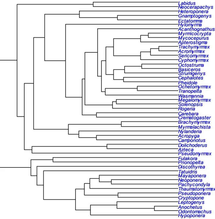
170 We produced a genus-level phylogenetic tree and calculated phylogenetic distances among all
171 inventoried genera (n = 56) using the phylogenetic tree produced in a recent publication
172 (Blanchard & Moreau 2016). Because two genera sampled in this study (Gigantiops and
173 Rasopone) were missing in the tree of Blanchard & Moreau (2016), our resulting tree contained 174 54 genera (Figure S1).
175
176 2.5. Environmental data
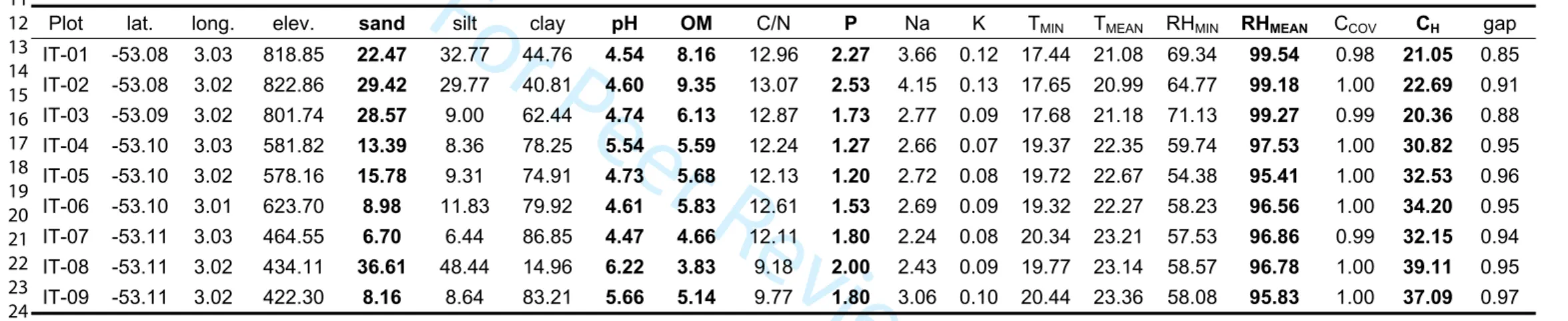
177 We measured environmental parameters from soil, climatic and LiDAR data.
178 2.5.1. Soil data
179 In each plot, soil samples were collected at ten locations from three different soil layers (0-10,
180 10-20, 20-30cm), following the procedure described in Baraloto et al. (2011). The 10 samples for
181 each depth were then bulked into a single composite sample of ca. 500g of soil. Composite
182 sample were then transported to the Laboratory Ecofog and dried to reach constant weight at
183 25°C, sieved to 2mm and sent to the INRA Arras soil analysis laboratory (Arras, France) for
184 physical and chemical analyses. A set of nine physico-chemical properties were measured (Table
185 S2): the percentage of sand, silt and clay, soil pH, the percentage of organic matter (OM), the
186 carbon-to-nitrogen ratio (C/N), and the soil P, Na and K contents. Particle size analysis of sand,
187 silt and clay were quantitatively performed by their settling rates in an aqueous solution using a
188 hydrometer. Soil pH was measured in 1 M potassium chloride solution. The organic matter
189 content was determined based on the loss of gases after ignition for 2h at 360°C. The total
190 amount of nitrogen (N) and carbon (C) in all forms in soil were quantitatively analyzed using a
191 dynamic flash combustion system coupled with a gas chromatographic separation system and
192 thermal conductivity detection system. Extractable Phosphorus (P) was assayed using the Olsen
193 method (Olsen et al. 1954) based on the extraction of phosphate from the soil by 0.5 N sodium
3 4 5 6 7 8 9 10 11 12 13 14 15 16 17 18 19 20 21 22 23 24 25 26 27 28 29 30 31 32 33 34 35 36 37 38 39 40 41 42 43 44 45 46 47 48 49 50 51 52 53 54 55 56 57
For Peer Review Only
194 bicarbonate solution adjusted to pH 8.5. A semi-quantitative method was used to determine the
195 amount of soil exchangeable sodium (Na) and potassium (K) residing on the soil colloid
196 exchange sites by displacement with ammonium acetate solution buffered to pH 7.0.
197
198 2.5.2. Climatic data
199 Air temperature (in °C) and relative humidity (in %) were measured in all plots using
micro-200 environmental sensors (HOBO U23-001) as described in Tymen et al. (2017). The weather
201 sensors were placed within the area of each plot except for Plot 6, for which the sensor was
202 placed halfway between Plot 5 and 6 because of a logistical issue. Since this sensor was not far
203 away for the sampled area and at the same elevation, the climatic data were used as a proxy for
204 environmental data of this plot (see Figure 1).
205 The two parameters (air temperature and relative humidity) were monitored for one year,
206 from 1 January 2015 to 31 December 2015 with one measurement every 30 minutes. Using the
207 local micro-environmental data, we defined four climatic variables for each plot (Table S2):
208 TMEAN – mean annual Temperature, RHMEAN – mean annual Relative Humidity, TMIN – minimum
209 temperature of the coldest month, RHMIN – minimum Relative Humidity of the driest month.
210
211 2.5.3. LiDAR data
212 LiDAR data were acquired in early August 2014 using a LMS-Q560 RIEGL laser range finder
213 (wave length 1550nm) on board an aircraft flying at ca. 600m above the ground. A total of 64
214 km2 were covered with a scan angle ranging from ± 25°. Point density slightly exceeded 20
215 pts/m2 (pulse density ca. 13 pulses/m2), with a ground point density of 0.31 pts/m2. Digital
216 Elevation Model (DEM) at 1m resolution was interpolated from ground LiDAR points using
217 Lastools (Insenburg n.d.). Digital Surface Model (DSM) was built using Quick Terrain Modeler
3 4 5 6 7 8 9 10 11 12 13 14 15 16 17 18 19 20 21 22 23 24 25 26 27 28 29 30 31 32 33 34 35 36 37 38 39 40 41 42 43 44 45 46 47 48 49 50 51 52 53 54 55 56 57
For Peer Review Only
218 (free trial version, http://appliedimagery.com) at the same resolution. Canopy Height Model
219 (CHM) was then calculated as the difference between DSM and DEM. When we
ground-220 surveyed our plots, multiple GPS point positions were acquired for each plot using a hand-held
221 GPS (accuracy 5–10m). To further improve plot geo-referencing, we adjusted plot locations
222 against LiDAR CHM as in Réjou-Méchain et al. (2015): the location of all surveyed trees (DBH
223 ≥ 30cm) inferred from ground positioning was first compared to that deduced from CHM. Tree
224 GPS coordinates were then shifted until best match with the CHM, resulting in horizontal shifts
225 typically of less than 15m. With the improved plot locations, we then derived three variables for
226 the plots from LiDAR data (Table S2): canopy height (CH), canopy cover (CCOV) and the gap
227 fraction (gap). Canopy height was calculated as the mean value of CHM pixels inside each plot.
228 Canopy cover was calculated using LAStools (lascanopy -cov), with the height threshold set at
229 5m for separating canopy and non-canopy points. Gap fraction was also calculated following the
230 approach of Morsdorf et al. (2006), which was defined as the percent of vegetation echoes to all
231 (ground and vegetation) echoes.
232
233 2.6. Data analysis
234 All analyses were conducted using R 3.5.1 statistical software (R Core Team 2018). The
235 taxonomic, functional and environmental datasets are available in supplementary material (Tables
236 S1, S2 and S3).
237
238 2.6.1. Functional heterogeneity among species
239 The mean value of traits (n = 9) per species were normalized by using a Box-Cox transformation,
240 then all traits (except Weber’s length) were standardized by dividing their values by Weber’s
241 length to correct for individual body size (see Table 1). A Principal Component Analysis (PCA)
3 4 5 6 7 8 9 10 11 12 13 14 15 16 17 18 19 20 21 22 23 24 25 26 27 28 29 30 31 32 33 34 35 36 37 38 39 40 41 42 43 44 45 46 47 48 49 50 51 52 53 54 55 56 57
For Peer Review Only
242 on the species × traits matrix (hereafter, PCATRAITS) was then performed to eliminate trait
243 redundancy (see Figure S2), using the R package “FactoMineR” (Lê et al. 2008). Subsequent
244 analyses were based on the first three principal components (except for the fourth-corner analysis
245 for which we also used individual traits; see below), which jointly explained 77% of the overall
246 trait inertia (Table S4).
247
248 2.6.2. Environmental heterogeneity among plots
249 Environmental variables were normalized (using Box-Cox transformation) and standardized
(z-250 score transformation) prior to analyses, using the R package “forecast” (Hyndman & Khandakar
251 2008, Hyndman et al. 2019). We then performed a PCA on all environmental variables (n = 17),
252 hereafter the PCAENV, to examine associations among variables and characterize environmental
253 differences among plots. The difference among the three elevations for each environmental
254 variable was tested using a Kruskal-Wallis test.
255
256 2.6.3. Community-wide taxonomic, functional and phylogenetic structure
257 A community that is taxonomically, functionally or phylogenetically clustered within plot
258 corresponds to a situation where species co-occurring within these plots share more similar taxa,
259 traits, or are phylogenetically closer-related, respectively, than species from different plots. This
260 clustering was quantified using the IST, τST and ПST statistics which calculate the taxonomic,
261 functional and phylogenetic turnover among plots, respectively (Hardy & Senterre 2007). The
262 three indices are calculated as followed:
263 IST = 1 - TDw/TDa (Taxonomic turnover) eq. 1
264 τST = 1 - FDw/FDa (Functional turnover) eq. 2
3 4 5 6 7 8 9 10 11 12 13 14 15 16 17 18 19 20 21 22 23 24 25 26 27 28 29 30 31 32 33 34 35 36 37 38 39 40 41 42 43 44 45 46 47 48 49 50 51 52 53 54 55 56 57
For Peer Review Only
265 ПST = 1 - PDw/PDa (Phylogenetic turnover) eq. 3
266 where TD corresponds to the Taxonomic Diversity calculated using Simpson index with species
267 occurrence data; FD and PD correspond, respectively, to the mean Functional Dissimilarity (here,
268 Euclidean) between distinct species and the mean Phylogenetic Distance (mean divergence time
269 based on the phylogenetic tree) between distinct genera (thus FD and PD are based on
270 species/genus presence-absence), within (w) and among (a) plots. τST and ПST thus quantify the
271 relative increase of the mean functional divergence and phylogenetic distance between species
272 sampled among plots versus within plots, respectively. Species, trait and phylogenetic clustering
273 is observed if IST, τST or ПST > 0, respectively, while negative values indicate overdispersion
274 (Hardy & Senterre 2007). The overall clustering within plot was calculated using the mean IST,
275 τST and ПST values among all pairs of plots. These mean values were tested by comparing their
276 observed value with 999 null values obtained under a null model where species occurrences are
277 randomized across plots (Hardy 2008). We then used the pairwise values of these statistics
278 among all pairs (n = 36) of different plots in regression models to test the effect of environmental
279 dissimilarity on taxonomic, functional and phylogenetic turnover (see next section). Turnover
280 values were also quantified and tested among pairs of altitudes (three comparisons, 400-600m,
281 400-800m and 600-800m). These indices were calculated using the R package “spacodiR”
282 (Eastman et al. 2013).
283
284 2.6.4. Environmental determinants of taxonomic, functional and phylogenetic composition
285 We used Multiple Regression on distance Matrices (MRM; Lichstein 2007) to quantify and test
286 the association between environmental dissimilarity and taxonomic (IST), phylogenetic (ПST) and
287 functional (τST) turnover of ant assemblages among plots, using the R package “ecodist” (Goslee
3 4 5 6 7 8 9 10 11 12 13 14 15 16 17 18 19 20 21 22 23 24 25 26 27 28 29 30 31 32 33 34 35 36 37 38 39 40 41 42 43 44 45 46 47 48 49 50 51 52 53 54 55 56 57
For Peer Review Only
288 & Urban 2007). Statistical significance of each regression coefficient was assessed through
289 residuals permutation tests (n = 9,999 permutations). Pairwise τST values corresponded more
290 exactly to the functional turnover among plots calculated using the three first axes of the
291 PCATRAITS together, as well as each of these axes individually. Analyzing the functional turnover
292 based on individual PCA axes can help identifying significant effects on traits that may be
293 obscured when all traits are taken into account in the analysis. The examination of trait loadings
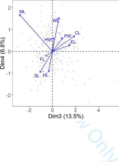
294 on the PCA axes can help identifying those traits (Figure 2). It is worth noting that all of our tests
295 may suffer from a limited statistical power due to the number of pairwise turnover values (n = 36)
296 investigated in the MRM. Thus, while the significant signals observed may reflect some
297 ecological reality, the absence of signals should also be taken with caution as they could mean
298 that our sampling design did not allow capturing a significant association.
299 Three types of MRM models were used for each of the six response variable (IST, τST
300 calculated over the three first axes of the PCATRAITS, τST calculated for each of these three axes,
301 and ПST). The first model (Model 1) corresponded to a simple regression testing the effect of the
302 overall environmental (Euclidean) dissimilarity (calculated over the 17 environmental variables)
303 on each response variable. Model 2 corresponded to a multiple regression model where we tested
304 the relative effects (regression coefficients) of the dissimilarity of several environmental
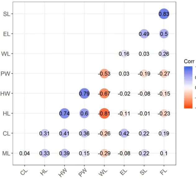
305 variables, using a reduced set of variables with limited collinearity to limit the number of tests.
306 To do so, we retained ecologically relevant variables with r-Spearman correlation ≤ 0.6 for
307 climate and soil variables separately (Figures S3-4). In doing so, four soil variables (the
308 percentage of sand, OM, soil pH and P) and one climatic variable (RHMEAN) were retained for
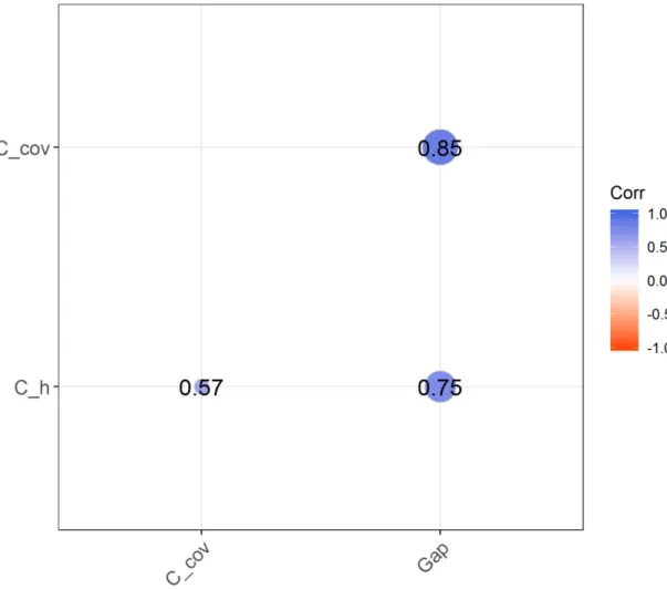
309 analyses. For LiDAR data, because the variation in the variables “canopy cover” and “gap
310 fraction” remained virtually unchanged across plots (see Table S2), we only retained the variable
311 “canopy height” (CH) for analyses. This latter variable was positively correlated to the variables
3 4 5 6 7 8 9 10 11 12 13 14 15 16 17 18 19 20 21 22 23 24 25 26 27 28 29 30 31 32 33 34 35 36 37 38 39 40 41 42 43 44 45 46 47 48 49 50 51 52 53 54 55 56 57
For Peer Review Only
312 “canopy cover” and “gap fraction” (Figure S5). In Model 3, we tested the relative effects of the
313 dissimilarity in the scores of the two first axes of the PCAENV. In each of the three models, the
314 spatial dependence among plots was taken into account by including spatial distance (Euclidean,
315 untransformed) among the explanatory variables.
316 Finally, to have more accurate insights regarding the associated pairs of environmental
317 variables and traits, we performed a fourth-corner analysis (Legendre et al. 1997), using the R
318 packages “ade4” (Dray & Dufour 2007) and “adespatial” (Dray et al. 2019). The fourth-corner
319 analysis combines three matrices – plots × environmental variables (R), plots × species
320 occurrences (L) and species × traits (Q) – into a matrix of trait-environment associations. The
321 latter is then used to quantify and test pairwise associations between traits and environmental
322 variables, using 9,999 randomizations with the so-called model “6” which combines models “2”
323 and “4” as described in Dray et al. (2014), in order to avoid type-I error inflation.
324
325 3. RESULTS
326
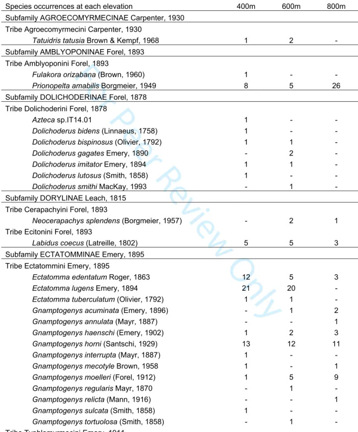
327 We collected a total of 31,865 ant individuals belonging to 267 species, 56 genera and 11
328 subfamilies along the elevational gradient at Mont Itoupé (Table S3). The total number of species
329 slightly decreased with increasing elevation (resp. 198, 176 and 161 species at 400m, 600m and
330 800m asl.). Across plots, the number of observed species ranged from 85 (P6; 600m asl.) to 129
331 (P9; 400m asl.). The average number of species per sample was higher at the lowest elevations
332 (400m: mean ± sd = 25.45 ± 2.69; 600m: mean ± sd = 20.38 ± 4.48; 800m: mean ± sd = 20.63 ±
333 1.60). We also calculated the Simpson’s index and found very similar values along the
334 elevational gradient (mean ± sd = 0.98 ± <0.01 for each elevation).
335 3 4 5 6 7 8 9 10 11 12 13 14 15 16 17 18 19 20 21 22 23 24 25 26 27 28 29 30 31 32 33 34 35 36 37 38 39 40 41 42 43 44 45 46 47 48 49 50 51 52 53 54 55 56 57
For Peer Review Only
336 3.1. Functional heterogeneity
337 The PCA performed on species traits (PCATRAITS) showed that the first three axes jointly
338 explained 77% of the overall trait inertia (38%, 26% and 13%, respectively; Figures 2 and S6;
339 Table S4). Plot scores on the first axis were highly positively correlated to HL, HW, PW and
340 negatively to WL. The second axis was mostly associated with FL, SL and EL which were highly
341 positively correlated to each other; the third axis was negatively associated to ML (Figures 2 and
342 S6, Table S4).
343
344 3.2. Environmental heterogeneity
345 The PCA performed on the matrix of environmental data (hereafter, PCAENV) revealed that axes
346 1 and 2 explained 60.5% and 20.7% of the overall environmental inertia across the nine plots,
347 respectively (Figure 3; Table S5). Among the variables retained for analyses, PCA scores
348 indicated that relative humidity (RHMEAN) and canopy height (CH) were strongly correlated to
349 axis 1 (resp. r = 0.93 and r = -0.90), while pH was strongly correlated to axis 2 (r = 0.85).
350 We found that the following variables significantly (or almost) varied across elevations
(Kruskal-351 Wallis rank tests): OM (X2 = 7.20, p = 0.03), C
H (X 2 = 6.00, p = 0.05), P (X 2 = 2.40, p = 0.06)
352 and RHMEAN (X 2 = 5.42, p = 0.07). In contrast, no significant variation was found in sand (X 2 =
353 2.40, p = 0.30) and soil pH (X 2 = 0.61, p = 0.74) across elevations.
354
355 3.3. Taxonomic, functional and phylogenetic structure of ant assemblages
356 The leaf-litter ant assemblages displayed significant taxonomic and trait clustering at the plot
357 level (Table 2). Trait clustering was mostly explained by a significant clustering observed for the
358 scores of the second axis of the PCATRAITS (Table 2), which accounted for 26% of the overall
359 functional inertia. The latter axis (i.e. axis 2 of the PCATRAITS) was mostly associated to relative
3 4 5 6 7 8 9 10 11 12 13 14 15 16 17 18 19 20 21 22 23 24 25 26 27 28 29 30 31 32 33 34 35 36 37 38 39 40 41 42 43 44 45 46 47 48 49 50 51 52 53 54 55 56 57
For Peer Review Only
360 femur and scape length (Figure 2; Table S4). In contrast, we did not find any significant
361 phylogenetic clustering (Table 2). We further found that the taxonomic clustering was mostly due
362 to differences in species composition between 800 and 600m-elevated plots, and that the
363 functional clustering was mostly due to differences in trait composition between the most
364 elevated plots (800m) and the other plots (Table 2). No phylogenetic clustering signal was found
365 at the plot or the elevation level.
366
367 3.4. Effect of environmental variables on taxonomic, functional and phylogenetic
368 composition
369 To facilitate the reading hereafter, we will sometimes omit to use the term “dissimilarity” when
370 describing that the “dissimilarity of A significantly explains the dissimilarity of B”, and will
371 simply write that “A significantly explains B” but we must keep in mind that we only deal with
372 dissimilarity values among plots in our regression models. The overall environmental
373 dissimilarity significantly explained the taxonomic (IST) and the overall functional (τST) turnover
374 among plots (Table 3) but not the phylogenetic (ПST) turnover. Moreover, the scores of the first
375 axis (strongly associated to the Weber’s length, the relative head length, the relative head width
376 and the pronotum width) and second axis (strongly associated to the relative scape and the
377 relative femur lengths) of the PCATRAITS were significantly explained by the overall
378 environmental dissimilarity.
379 Meanwhile, the plot scores of the first axis of the PCAENV (which was strongly associated
380 with temperature, relative humidity and vegetation structure; Table S5) significantly explained
381 the variation in the overall taxonomic and functional composition, as well as the variation in the
382 plot scores of axes 1 and 2 of the PCATRAITS (Table 3). When examining the relative effects of
383 each of the six selected environmental variable (sand, pH, OM, P, RHMEAN and CH), we found
3 4 5 6 7 8 9 10 11 12 13 14 15 16 17 18 19 20 21 22 23 24 25 26 27 28 29 30 31 32 33 34 35 36 37 38 39 40 41 42 43 44 45 46 47 48 49 50 51 52 53 54 55 56 57
For Peer Review Only
384 that soil phosphorus content and canopy height significantly explained the taxonomic
385 composition (IST) but not the overall functional composition (τST), the latter being only explained
386 by the percentage of sand (with a marginal significance; p = 0.081). Although the second axis of
387 the PCATRAITS displayed the strongest association with environment and with the first axis of the
388 PCAENV, it was not significantly explained by any individual environmental variable, despite a
389 relatively high coefficient value obtained with CH, which may result from a lack of power. Axis 1
390 and 3 of the PCATRAITS, however, were both significantly explained by soil phosphorus, while
391 axis 1 was also significantly explained by pH and axis 3 by the percentage of sand. The
392 phylogenetic (ПST) turnover was (marginally) significantly explained by soil pH only.
393 The fourth-corner analysis indicated that the percentage of sand was negatively related to
394 the relative scape, eye and femur lengths, and to the second and third axes of the PCATRAITS
395 (Table 4) which were highly associated to the variation of these three traits, while the third axis
396 was also strongly correlated to the relative mandible length (Table S4). Phosphorus concentration
397 was positively related to relative head length, whereas it was negatively related to Weber’s length
398 and the first axis of the PCATRAITS. Mean annual relative humidity was negatively related to
399 relative scape, eye and femur lengths of ants (Table 4).
400
401 4. DISCUSSION
402
403 This study highlights the existence of associations between key abiotic environmental variables
404 and the distribution of species and functional traits among Neotropical ant assemblages at a local
405 (i.e. 10km²) scale. Ant species and functional composition were mostly explained by canopy
406 height and the first axis of the PCAENV which was strongly associated to the relative humidity
407 and temperature (and thus elevation), and to a lesser extent by soil phosphorus concentration,
3 4 5 6 7 8 9 10 11 12 13 14 15 16 17 18 19 20 21 22 23 24 25 26 27 28 29 30 31 32 33 34 35 36 37 38 39 40 41 42 43 44 45 46 47 48 49 50 51 52 53 54 55 56 57
For Peer Review Only
408 sand and pH (Table 3). The observed within-plot and within-elevation functional clustering
409 (Table 2) likely arose from the filtering of these environmental conditions.
410 Climate represents a major environmental filter and restricts the number and identity of
411 species that can survive and establish at different locations. Among climatic filters, temperature
412 has been shown to be a key parameter influencing patterns of ant species distributions (e.g.
413 Sanders et al. 2007, Dunn et al. 2009, Silva & Brandão 2014). Other studies have also reported a
414 relationship between temperature and ant functional composition (Stuble et al. 2013, Arnan et al.
415 2014). Relative humidity may be even more constraining for leaf-litter ants than temperature
416 (Kaspari & Weiser 2000, Menke & Holway 2006). These studies reported results that were
417 consistent with our findings. Indeed, we found that the variation in the dissimilarity of plot scores
418 along the first axis of the PCAENV, which was highly explained by variation in soil relative
419 humidity, temperature and elevation (Figure 3; Table S5), significantly explained the taxonomic
420 and functional turnover. As highlighted by the PCA generated on environmental data (PCAENV;
421 Figure 3), the top of the mountain (ca. 800m asl), which is covered by cloud forests, is
422 characterized by slightly higher levels of humidity (meanRH = 99.3%) compared to lower
423 elevations (between ca. 400 and 600m asl; meanRH = 96.5%). The top forests may therefore
424 provide a refuge area for certain species preferring relatively colder and more humid conditions.
425 Changes in species and functional composition may thus reflect the presence of
climate-426 specialists at higher elevations. More specifically, our results suggest that smaller ant species, as
427 well as species with relative smaller eyes or smaller legs, were found in sites with higher levels of
428 humidity (thus at higher elevation). These traits are characteristics of hypogaeic ant species, i.e.
429 ant species that nest and forage within the litter or into the soil (Weiser & Kaspari 2006).
430 Along Mont Itoupé, turnovers in species and functional composition were also associated to
431 variation in phosphorus concentration (Table 3). Phosphorus limitation may explain variation in
3 4 5 6 7 8 9 10 11 12 13 14 15 16 17 18 19 20 21 22 23 24 25 26 27 28 29 30 31 32 33 34 35 36 37 38 39 40 41 42 43 44 45 46 47 48 49 50 51 52 53 54 55 56 57
For Peer Review Only
432 plant diversity (Wright et al. 2011, Vleminckx et al. 2017), which in turn is likely to influence the
433 diversity and density of leaf-litter associated invertebrates (McGlynn & Salinas 2007, Vleminckx
434 et al. 2019). In their study, McGlynn and Salinas (2007) found that environments richer in 435 phosphorus had greater litter invertebrate densities (mostly detritivores). Thus, the association
436 between phosphorus availability and the species and functional composition of ant communities
437 may be indirectly explained by the variation in the density of prey for predatory ant species. The
438 fourth-corner analysis performed in this study reveal that phosphorus concentration was
439 positively related to the relative head length and negatively related to body length (i.e. Weber’s
440 length), features that are characteristics of small hypogaeic ant species belonging to genera such
441 as Carebara, Solenopsis and Strumigenys. Those predatory ant genera may thus benefit from the
442 higher phosphorus concentrations that may favor the abundance of small prey. Such results
443 contrast with those obtained in a study conducted by Jacquemin et al. (2012) in which they found
444 a decrease of predatory ant species in plots enriched in Carbon, Nitrogen and Phosphorus. In their
445 study, predatory ants seemed to be limited by habitat loss due to the increased litter
446 decomposition. The positive effect of higher levels of phosphorus for small predatory ant species
447 found in our study may have been counterbalanced by habitat loss in their study, since the
448 amount of leaf litter at the highest elevation, i.e. at high levels of phosphorus, was much more
449 important than at the lowest ones.
450 In addition to climatic factors, nutrient availability and soil texture can also influence
451 invertebrate composition by imposing constraints on species living in ground habitats
452 (Vasconcelos et al. 2003, Schmidt et al. 2016, Costa-Milanez et al. 2017), but also indirectly via
453 an effect of these variables on tree community assembly (Vleminckx et al. 2019). In our study, a
454 significant association was found between the functional composition and the soil texture
455 (percentage of sand) turnover across plots (Table 3), especially for the third axis of the PCATRAITS
3 4 5 6 7 8 9 10 11 12 13 14 15 16 17 18 19 20 21 22 23 24 25 26 27 28 29 30 31 32 33 34 35 36 37 38 39 40 41 42 43 44 45 46 47 48 49 50 51 52 53 54 55 56 57
For Peer Review Only
456 which was mostly associated with the relative mandible length (Table S4). We lack hypotheses to
457 explain that result. In addition, the percentage of sand was negatively related to individual
458 functional traits of ants (i.e. the relative scape and femur lengths). Particular functional traits of
459 ant species rather than the global functional space of ant assemblages may thus be linked to soil
460 texture. Short scape and eye, relative to body size, are typical of hypogaeic ant species (Brandão
461 et al. 2012), foraging and nesting inside the leaf-litter. Sandy soils may thus favor movements 462 and nest establishment of hypogaeic species within the litter, compared to clay-rich soils.
463
464 CONCLUSIONS
465
466 Elevational gradients stretching from lowland forests to lower mountain cloud forests represent a
467 major source of environmental variation in tropical regions which, in our study, has been shown
468 to influence the distribution of leaf-litter ants. In particular, the taxonomic and functional
469 turnover of ant communities were mostly explained by soil phosphorus content, climatic
470 (temperature, relative humidity) variables and vegetation structure, while trait variation seemed to
471 be also influenced by soil texture and pH. Our results shed light on the unique biodiversity value
472 of cloud forests, a particularly rare ecosystem in the eastern Guiana Shield, likely to be threatened
473 by climate change, with scenarios predicting an intensification of drought events and an increase
474 of temperature across the region (Esquivel-Muelbert et al. 2019). Indeed, the congruence between
475 species and functional turnover along the humidity gradient highlights that a loss of species and
476 functional diversity represent real threats in this regional biodiversity hotspot.
477 478 ACKNOWLEDGMENTS 479 3 4 5 6 7 8 9 10 11 12 13 14 15 16 17 18 19 20 21 22 23 24 25 26 27 28 29 30 31 32 33 34 35 36 37 38 39 40 41 42 43 44 45 46 47 48 49 50 51 52 53 54 55 56 57
For Peer Review Only
480 We thank Sandrine Etienne for her work on the process of molecular data, and Aurélie Dourdain
481 for producing the map of the site. Thanks are also due to the national park managers for allowing
482 our research program in the core area of the Parc Amazonien de Guyane. Financial support for this
483 study was provided by an Investissement d’Avenir grant of the Agence Nationale de la Recherche
484 (CEBA, ANR-10-LABX-25-01) through a PhD fellowship to MF and the funding of the
485 DIADEMA (DIssecting Amazonian Diversity by Enhancing a Multiple taxonomic-groups
486 Approach) and DIAMOND (DIssecting And MONitoring amazonian Diversity) projects, by the
487 Programme Convergence 2007-2013, Région Guyane from the European community (BREGA, 488 757/2014/SGAR/DE/BSF) and by the PO-FEDER 2014-2020, Région Guyane (BiNG,
489 GY0007194).
490
491 DATA AVAILABILITY
492 Data available from the Dryad Digital Repository: https://doi.org/10.5061/dryad.00000 (Fichaux
493 et al. 2020). 494 495 496 497 REFERENCES 498
499 AGOSTI,D., and L.ALONSO. 2000. The ALL Protocol. In D. Agosti, J. Majer, L. Alonso, and T.
500 Schultz (Eds.) Ants: standard methods for measuring and monitoring biodiversity. pp. 204–206,
501 Washington D.C. USA.
502 ARNAN, X., X. CERDÁ, and J. RETANA. 2014. Ant functional responses along environmental
503 gradients. Journal of Animal Ecology 83: 1398–1408.
3 4 5 6 7 8 9 10 11 12 13 14 15 16 17 18 19 20 21 22 23 24 25 26 27 28 29 30 31 32 33 34 35 36 37 38 39 40 41 42 43 44 45 46 47 48 49 50 51 52 53 54 55 56 57
For Peer Review Only
504 ARNAN,X., X.CERDÁ, and J.RETANA. 2015. Partitioning the impact of environment and spatial
505 structure on alpha and beta components of taxonomic, functional, and phylogenetic diversity in
506 European ants. PeerJ 3: e1241.
507 BARALOTO, C., S. RABAUD, Q. MOLTO, L. BLANC, C. FORTUNEL, B. HÉRAULT, N. DÁVILA, I.
508 MESONES, M. RIOS, E. VALDERRAMA, and P. V. A. FINE. 2011. Disentangling stand and
509 environmental correlates of aboveground biomass in Amazonian forests. Global Change Biology
510 17: 2677–2688.
511 BESTELMEYER,B.T., D.AGOSTI, L.E. ALONSO, C.R.F.BRANDÃO, W. L.BROWN JR., J.H. C.
512 DELABIE, and R. SILVESTRE. 2000. Field techniques for the study of ground-dwelling ants: an
513 overview, description, and evaluation. In D. Agosti, J. Majer, L. Alonso, and T. Schultz (Eds.)
514 Ants: standard methods for measuring and monitoring biodiversity. pp. 122–144, Washington D.C.
515 USA.
516 BIHN,J.H., G.GEBAUER, and R.BRANDL. 2010. Loss of functional diversity of ant assemblages in
517 secondary tropical forests. Ecology 91: 782–792.
518 BISHOP,T.R., M.P.ROBERTSON, B.J. VAN RENSBURG, and C.L.PARR. 2015. Contrasting species
519 and functional beta diversity in montane ant assemblages. Journal of Biogeography 42: 1776–1786.
520 BLANCHARD,B.D., and C.S.MOREAU. 2016. Defensive traits exhibit an evolutionary trade-off
521 and drive diversification in ants. Evolution 71: 315–328.
522 BLATRIX, R., C. LEBAS, C. GALKOWSKI, P. WEGNEZ, R. PIMENTA, and D. MORICHON. 2016.
523 Vegetation cover and elevation drive diversity and composition of ant communities (Hymenoptera:
524 Formicidae) in a Mediterranean ecosystem. Myrmecological News 22: 119–127.
525 BRANDÃO,C.R. F., R.R.SILVA, and J. H. C.DELABIE. 2012. Neotropical ants (Hymenoptera)
526 functional groups: nutritional and applied implications. In J. R. P. Parra (Ed.) Insect bioecology
527 and nutrition for integrated pest management. pp. 213–236, CRC, Boca Raton.
3 4 5 6 7 8 9 10 11 12 13 14 15 16 17 18 19 20 21 22 23 24 25 26 27 28 29 30 31 32 33 34 35 36 37 38 39 40 41 42 43 44 45 46 47 48 49 50 51 52 53 54 55 56 57
For Peer Review Only
528 BRÜHL,C.A., M.MOHAMED, and K.E. LINSENMAIR. 1999. Altitudinal distribution of leaf litter
529 ants along a transect in primary forests on Mount Kinabalu, Sabah, Malaysia. Journal of Tropical
530 Ecology 15: 265–277.
531 CHEN,X., B.ADAMS, C.BERGERON, A.SABO, and L.HOOPER-BÙI. 2015. Ant community structure
532 and response to disturbances on coastal dunes of Gulf of Mexico. Journal of Insect Conservation
533 19: 1–13.
534 COSTA-MILANEZ,C.B. DA, J.D.MAJER, P. DE T.A.CASTRO, and S.P.RIBEIRO. 2017. Influence of
535 soil granulometry on average body size in soil ant assemblages: implications for bioindication.
536 Perspectives in Ecology and Conservation 15: 102–108.
537 DAVIDSON,D.W., S.C.COOK, and R.R.SNELLING. 2004. Liquid-feeding performances of ants
538 (Formicidae): ecological and evolutionary implications. Oecologia 139: 255–266.
539 DEHLING,D.M., S. A.FRITZ, T.TÖPFER, M.PÄCKERT, P.ESTLER, K.BÖHNING-GAESE, and M.
540 SCHLEUNING. 2014. Functional and phylogenetic diversity and assemblage structure of frugivorous
541 birds along an elevational gradient in the tropical Andes. Ecography 37: 1047–1055.
542 DEL TORO,I., R.R.RIBBONS, and S.L.PELINI. 2012. The little things that run the world revisited:
543 a review of ant-mediated ecosystem services and disservices (Hymenoptera: Formicidae).
544 Myrmecological News 17: 133–146.
545 DRAY, S., and A.-B. DUFOUR. 2007. The ade4 package: implementing the duality diagram for
546 ecologists. Journal of Statistical Software 22: 1–20.
547 DRAY,S., P.CHOLER, S.DOLÉDEC, P.R.PERES-NETO, W.THUILLER, S.PAVOINE, and C.J.F.TER
548 BRAAK. 2014. Combining the fourth-corner and the RLQ methods for assessing trait responses to
549 environmental variation. Ecology 95: 14–21.
550 DRAY,S., D. BAUMAN, G. BLANCHET, D. BORCARD, S. CLAPPE, G. GUENARD, T.JOMBART, G.
551 LAROCQUE, P.LEGENDRE, N.MADI, and H.H.WAGNER. 2019. adespatial: multivariate multiscale
3 4 5 6 7 8 9 10 11 12 13 14 15 16 17 18 19 20 21 22 23 24 25 26 27 28 29 30 31 32 33 34 35 36 37 38 39 40 41 42 43 44 45 46 47 48 49 50 51 52 53 54 55 56 57
For Peer Review Only
552 spatial analysis. R package version 0.3-4, https://CRAN.R-project.org/package=adespatial.
553 DUNN,R.R. ET AL. 2009. Climatic drivers of hemispheric asymmetry in global patterns of ant
554 species richness. Ecology Letters 12: 324–333.
555 EASTMAN, J., T. PAINE, and O. HARDY. 2013. spacodiR: spatial and phylogenetic analysis of
556 community diversity. R package version 0.13-0115,
https://CRAN.R-557 project.org/package=spacodiR.
558 ESQUIVEL‐MUELBERT, A. ET AL. 2019. Compositional response of Amazon forests to climate
559 change. Global Change Biology 25: 39–56.
560 FEENER JR., D. H., J. R. B. LIGHTON, and G. A. BARTHOLOMEW. 1988. Curvilinear allometry,
561 energetics and foraging ecology: a comparison of leaf-cutting ants and army ants. Functional
562 Ecology 2: 509–520.
563 FICHAUX,M.,B.BÉCHADE,J.DONALD,A.WEYNA,J.H.C.DELABIE,J.MURIENNE,C.BARALOTO,
564 and J. ORIVEL.2019. Habitats shape taxonomic and functional composition of Neotropical ant
565 assemblages. Oecologia 189: 201–513.
566 FICHAUX,M.,J.VLEMINCKX,E.A.COURTOIS,J.H.CDELABIE,J.GALLI,S.TAO,N.LABRIÈRE,J.
567 CHAVE,C.BARALOTO,J.ORIVEL. 2020. Data from: Environmental determinants of leaf-litter ant
568 community composition along an elevational gradient. Dryad Digital Repository. 569 doi:10.5061/dryad.00000
570 FOLGARAIT,P.J. 1998. Ant biodiversity and its relationship to ecosystem functioning: a review.
571 Biodiversity and Conservation 7: 1221–1244.
572 FONTANILLA,A.M., A.NAKAMURA, Z.XU, M.CAO, R.L.KITCHING, Y.TANG, and C.J.BURWELL.
573 2019. Taxonomic and functional ant diversity along tropical, subtropical, and subalpine elevational
574 transects in Southwest China. Insects 128.
3 4 5 6 7 8 9 10 11 12 13 14 15 16 17 18 19 20 21 22 23 24 25 26 27 28 29 30 31 32 33 34 35 36 37 38 39 40 41 42 43 44 45 46 47 48 49 50 51 52 53 54 55 56 57
For Peer Review Only
575 FOWLER,H.G., L.C.FORTI, C.R.F.BRANDÃO, J.H.C.DELABIE, and H.L.VASCONCELOS. 1991.
576 Ecologia nutricional de formigas. In A. R. Panizzi and J. R. P. Parra (Eds.) Ecologia nutricional de
577 insetos e suas implicaçoes no manejo de pragas. pp. 131–223, São Paulo, Brazil: Editora Manole.
578 GOSLEE,S.C., and D.L. URBAN. 2007. The ecodist package for dissimilarity-based analysis of
579 ecological data. Journal of Statistical Software 22: 1–19.
580 GOTELLI,N.J. 2000. Null model analysis of species co-occurrence patterns. Ecology 81: 2606–
581 2621.
582 GRAHAM, C.H., J. L. PARRA, C. RAHBEK, and J. A. MCGUIRE. 2009. Phylogenetic structure in
583 tropical hummingbird communities. Proceedings of the National Academy of Sciences 106:
584 19673–19678.
585 GROC,S., J.ORIVEL, A.DEJEAN,J.-M.MARTIN,M.-P.ETIENNE,B.CORBARA , andJ.H.C.DELABIE.
586 2009. Baseline study of the leaf‐litter ant fauna in a French Guianese forest. Insect Conservation
587 and Diversity 2: 183–193.
588 GROC, S., J. H. C. DELABIE, F. FERNÁNDEZ, M. LEPONCE, J. ORIVEL, R. SILVESTRE, H. L.
589 VASCONCELOS, and A.DEJEAN. 2014. Leaf-litter ant communities (Hymenoptera: Formicidae) in
590 a pristine Guianese rain-forest: Stable functional structure versus high species turnover.
591 Myrmecological News 19: 43–51.
592 GRONENBERG,W., J.TAUTZ, and B.HÖLLDOBLER. 1993. Fast trap jaws and giant neurons in the
593 ant Odontomachus. Science 262: 561–563.
594 HARDY,O. J. 2008. Testing the spatial phylogenetic structure of local communities: Statistical
595 performances of different null models and test statistics on a locally neutral community. Journal of
596 Ecology 96: 914–926.
597 HARDY,O.J., and B.SENTERRE. 2007. Characterizing the phylogenetic structure of communities
598 by an additive partitioning of phylogenetic diversity. Journal of Ecology 95: 493–506.
3 4 5 6 7 8 9 10 11 12 13 14 15 16 17 18 19 20 21 22 23 24 25 26 27 28 29 30 31 32 33 34 35 36 37 38 39 40 41 42 43 44 45 46 47 48 49 50 51 52 53 54 55 56 57
For Peer Review Only
599 HE,X., E. HOU, Y.LIU, and D. WEN. 2016. Altitudinal patterns and controls of plant and soil
600 nutrient concentrations and stoichiometry in subtropical China. Scientific Reports 6: 24261.
601 HELMER,E.H., E.A.GERSON, L.S.BAGGETT, B.J.BIRD, T.S.RUZYCKI, and S.M.VOGGESSER.
602 2019. Neotropical cloud forests and páramo to contract and dry from declines in cloud immersion
603 and frost S. Lötters (Ed.). PLoS ONE 14: e0213155.
604 HILLEBRAND, H. 2004. On the generality of the latitudinal diversity gradient. The American
605 Naturalist 163: 192–211.
606 HODKINSON, I. D. 2005. Terrestrial insects along elevation gradients: species and community
607 responses to altitude. Biological Reviews 80: 489–513.
608 HOISS,B., J.KRAUSS, S.G.POTTS, S.ROBERTS, and I.STEFFAN-DEWENTER. 2012. Altitude acts as
609 an environmental filter on phylogenetic composition, traits and diversity in bee communities.
610 Proceedings of the Royal Society B: Biological Sciences 279: 4447–4456.
611 HÖLLDOBLER,B., and E.O.WILSON. 1990. The Ants. Harvard University Press.
612 HYNDMAN, R. J., and Y. KHANDAKAR. 2008. Automatic time series forecasting: the forecast
613 package for R. Journal of Statistical Software 27: 1–23.
614 HYNDMAN,R., G.ATHANASOPOULOS, C.BERGMEIR, G.CACERES, L.CHHAY, M.O’HARA-WILD,
615 F.PETROPOULOS, S.RAZBASH, E.WANG, and F.YASMEEN. 2019. forecast: forecasting functions
616 for time series and linear models. R package version 8.7, <URL:
617 http://pkg.robjhyndman.com/forecast>.
618 INSENBURG, M. LAStools—efficient LiDAR processing software (version 160921, academic)
619 obtained from http://rapidlasso.com/LAStools.
620 JACQUEMIN,J.,M.MARAUN,Y.ROISIN,and M. LEPONCE. 2012. Differential response of ants to
621 nutrient addition in a tropical Brown Food Web. Soil Biology and Biochemistry 46: 10–17.
622 KASPARI,M. 1993. Body size and microclimate use in Neotropical granivorous ants. Oecologia 96:
3 4 5 6 7 8 9 10 11 12 13 14 15 16 17 18 19 20 21 22 23 24 25 26 27 28 29 30 31 32 33 34 35 36 37 38 39 40 41 42 43 44 45 46 47 48 49 50 51 52 53 54 55 56 57
For Peer Review Only
623 500–507.
624 KASPARI,M., and M.D.WEISER. 1999. The size–grain hypothesis and interspecific scaling in ants.
625 Functional Ecology 13: 530–538.
626 KASPARI,M., and M. D.WEISER. 2000. Ant activity along moisture gradients in a Neotropical
627 forest. Biotropica 32: 703–711.
628 KEDDY,P.A. 1992. Assembly and response rules: two goals for predictive community ecology.
629 Journal of Vegetation Science 3: 157–164.
630 KOCHER,A., J.-C.GANTIER, P.GABORIT, L. ZINGER, H. HOLOTA, S. VALIERE, I. DUSFOUR, R.
631 GIROD, A. L. BAÑULS, and J.MURIENNE. 2016. Vector soup: high-throughput identification of
632 Neotropical phlebotomine sand flies using metabarcoding. Molecular Ecology Resources 17: 172–
633 182.
634 KRAFT,N.J.B., L.S.COMITA, J.M.CHASE, N.J.SANDERS, N.G. SWENSON, T.O.CRIST, J.C.
635 STEGEN, M. VELLEND, B. BOYLE, M. J. ANDERSON, H. V. CORNELL, K. F. DAVIES, A. L.
636 FREESTONE, B. D. INOUYE, S. P.HARRISON, and MYERS. 2011. Disentangling the drivers of β
637 diversity along latitudinal and elevational gradients. Science 1755–1758.
638 LÊ,S., J.JOSSE, and F.HUSSON. 2008. FactoMineR: an R package for multivariate analysis. Journal
639 of Statistical Software 25: 1–18.
640 LEGENDRE, P., R. GALZIN, and M. L. HARMELIN-VIVIEN. 1997. Relating behavior to habitat:
641 solutions to the fourth-corner problem. Ecology 78: 547–562.
642 LICHSTEIN,J.W. 2007. Multiple regression on distance matrices: a multivariate spatial analysis
643 tool. Plant Ecology 188: 117–131.
644 LONGINO,J.T., M.G.BRANSTETTER, and R.K.COLWELL. 2014. How ants drop out: ant abundance
645 on tropical mountains. PloS one 9: e104030.
646 LOS, S.O., F. A. STREET-PERROTT, N.J. LOADER, C.A. FROYD, A.CUNÍ-SANCHEZ, and R. A.
3 4 5 6 7 8 9 10 11 12 13 14 15 16 17 18 19 20 21 22 23 24 25 26 27 28 29 30 31 32 33 34 35 36 37 38 39 40 41 42 43 44 45 46 47 48 49 50 51 52 53 54 55 56 57
For Peer Review Only
647 MARCHANT. 2019. Sensitivity of a tropical montane cloud forest to climate change, present, past
648 and future: Mt. Marsabit, N. Kenya. Quaternary Science Reviews 218: 34–48.
649 MACHAC, A., M. JANDA, R. R. DUNN, and N. J. SANDERS. 2011. Elevational gradients in
650 phylogenetic structure of ant communities reveal the interplay of biotic and abiotic constraints on
651 diversity. Ecography 34: 364–371.
652 MCCAIN, C. M., and J.-A. GRYTNES. 2010. Elevational gradients in species richness. In
653 Encyclopedia of Life Sciences (ELS). pp. 1–10, John Wiley & Sons, Ltd, Chichester, UK.
654 MCGLYNN, T. P., and D. J. SALINAS. 2007. Phosphorus limits tropical rain forest litter fauna.
655 Biotropica 39: 50–53.
656 MENKE,S.B., and D.A.HOLWAY. 2006. Abiotic factors control invasion by Argentine ants at the
657 community scale. Journal of Animal Ecology 75: 368–376.
658 MORSDORF,F., B.KÖTZ, E.MEIER, K.I.ITTEN, and B.ALLGÖWER. 2006. Estimation of LAI and
659 fractional cover from small footprint airborne laser scanning data based on gap fraction. Remote
660 Sensing of Environment 104: 50–61.
661 NOWROUZI,S.,A.A.ANDERSEN,S.MACFADYEN,K.M.STAUNTON,J.VANDERWAL,and S.K.A.
662 ROBSON. 2016. Ant diversity and distribution along elevational gradients in the Australian wet
663 tropics: the importance of seasonal moisture stability. PloS ONE 11: e0153420.
664 OLSEN S.,C.COLE,F.WATANABE,and L.DEAN.1954. Estimation of available phosphorus in soils
665 by extraction with sodium bicarbonate. USDA Circular Nr 939, US Gov. Print. Office,
666 Washington, D.C.
667 PURSCHKE,O., B.C.SCHMID, M.T.SYKES, P.POSCHLOD, S.G.MICHALSKI, W.DURKA, I.KÜHN,
668 M. WINTER, and H. C. PRENTICE. 2013. Contrasting changes in taxonomic, phylogenetic and
669 functional diversity during a long-term succession: insights into assembly processes. Journal of
670 Ecology 101: 857–866. 3 4 5 6 7 8 9 10 11 12 13 14 15 16 17 18 19 20 21 22 23 24 25 26 27 28 29 30 31 32 33 34 35 36 37 38 39 40 41 42 43 44 45 46 47 48 49 50 51 52 53 54 55 56 57
For Peer Review Only
671 RCORE TEAM. 2018. R: A Language and Environment for Statistical Computing.
672 RÉJOU-MÉCHAIN,M., B.TYMEN, L.BLANC, S.FAUSET, T.R.FELDPAUSCH, A.MONTEAGUDO, O.
673 L.PHILLIPS, H.RICHARD, and J.CHAVE. 2015. Using repeated small-footprint LiDAR acquisitions
674 to infer spatial and temporal variations of a high-biomass Neotropical forest. Remote Sensing of
675 Environment 169: 93–101.
676 SANDERS,N.J., J.-P.LESSARD, M.C.FITZPATRICK, and R.R.DUNN. 2007. Temperature, but not
677 productivity or geometry, predicts elevational diversity gradients in ants across spatial grains.
678 Global Ecology and Biogeography 16: 640–649.
679 SCHMIDT, F. A., J. H. SCHOEREDER, and M. D. N. CAETANO. 2016. Ant assemblage and
680 morphological traits differ in response to soil compaction. Insectes Sociaux 64: 219–225.
681 SILVA,R.R., and C.R.F.BRANDÃO. 2014. Ecosystem-wide morphological structure of leaf-litter
682 ant communities along a tropical latitudinal gradient. PLoS ONE 9: e93049.
683 SMITH,M.A., W.HALLWACHS, and D.H.JANZEN. 2014. Diversity and phylogenetic community
684 structure of ants along a Costa Rican elevational gradient. Ecography 37: 720–731.
685 STUBLE,K.L., S.L.PELINI, S.E.DIAMOND, D.A.FOWLER, R.R.DUNN, and N.J.SANDERS. 2013.
686 Foraging by forest ants under experimental climatic warming: a test at two sites. Ecology and
687 Evolution 3: 482–491.
688 SWENSON, N. G., P. ANGLADA-CORDERO, and J. A. BARONE. 2011. Deterministic tropical tree
689 community turnover: evidence from patterns of functional beta diversity along an elevational
690 gradient. Proc. R. Soc. B. 278: 1707.
691 TYMEN,B.,G.VINCENT,E.A.COURTOIS,J.HEURTEBIZE,J.DAUZAT,I.MARECHAUX,and J.CHAVE.
692 2017. Quantifying micro-environmental variation in tropical rainforest understory at landscape
693 scale by combining airborne LiDAR scanning and a sensor network. Annals of Forest Science 74:
694 32. 3 4 5 6 7 8 9 10 11 12 13 14 15 16 17 18 19 20 21 22 23 24 25 26 27 28 29 30 31 32 33 34 35 36 37 38 39 40 41 42 43 44 45 46 47 48 49 50 51 52 53 54 55 56 57
For Peer Review Only
695 VASCONCELOS,H.L., A.C.C.MACEDO, and J.M.S.VILHENA. 2003. Influence of topography on
696 the distribution of ground-dwelling ants in an Amazonian forest. Studies on Neotropical Fauna and
697 Environment 38: 115–124.
698 VLEMINCKX, J., J.-L. DOUCET, J. MORIN-RIVAT, A. B. BIWOLÉ, D. BAUMAN, O. J. HARDY, A.
699 FAYOLLE,J.-F.GILLET,K. DAÏNOU,A.GOREL and T.DROUET. 2017. The influence of spatially
700 structured soil properties on tree community assemblages at a landscape scale in the tropical forests
701 of southern Cameroon. Journal of Ecology 105: 354–366.
702 VLEMINCKX, J., H. SCHIMANN, T. DECAËNS, M. FICHAUX, V. VEDEL, G. JAOUEN, M. ROY, E.
703 LAPIED,J.ENGEL,A.DOURDAIN,P.PETRONELLI,J.ORIVEL and C.BARALOTO.2019. Coordinated
704 community structure among trees, fungi and invertebrate groups in Amazonian rainforests.
705 Scientific reports 9: 11337.
706 WEBER,N.A. 1938. The biology of the fungus-growing ants. Part 4. Additional new forms. Part 5.
707 The Attini of Bolivia. Revista de Entomologia 7: 154–206.
708 WEISER,M.D., and M.KASPARI. 2006. Ecological morphospace of New World ants. Ecological
709 Entomology 31: 131–142.
710 WILLIG,M.R., D.M.KAUFMAN, and R.D.STEVENS. 2003. Latitudinal gradients of biodiversity:
711 pattern, process, scale, and synthesis. Annual Review of Ecology, Evolution, and Systematics 34:
712 273–309.
713 WRIGHT,S.K.,J.B.YAVITT,N.WURZBURGER,B.L.TURNER,E.V.J.TANNER,E.J.SAYER,L.S.
714 SANTIAGO, M. KASPARI,L. O. HEDIN, K. E. HARMS, M. N.GARCIA, and M. D. CORRE. 2011.
715 Potassium, phosphorus, or nitrogen limit root allocation, tree growth, or litter production in a
716 lowland tropical forest. Ecology 92: 1616–1625.
717 YATES, M., H. GIBB, and N. R. ANDREW. 2011. Habitat characteristics may override climatic
718 influences on ant assemblage composition: A study using a 300-km climatic gradient climatic
3 4 5 6 7 8 9 10 11 12 13 14 15 16 17 18 19 20 21 22 23 24 25 26 27 28 29 30 31 32 33 34 35 36 37 38 39 40 41 42 43 44 45 46 47 48 49 50 51 52 53 54 55 56 57
For Peer Review Only
719 gradient. Australian Journal of Entomology 59: 332–338.
720 YATES,M.L., N.R.ANDREW, M. BINNS, and H.GIBB. 2014. Morphological traits: predictable
721 responses to macrohabitats across a 300 km scale. PeerJ 2: e271.
722 3 4 5 6 7 8 9 10 11 12 13 14 15 16 17 18 19 20 21 22 23 24 25 26 27 28 29 30 31 32 33 34 35 36 37 38 39 40 41 42 43 44 45 46 47 48 49 50 51 52 53 54 55 56 57