Adaptive changes in the morphology of natural materials due to alterations in mechanical stress

Adaptive Changes in the Morphology of Natural Materials Due to Alterations in Mechanical Stress

by

Katharine I. Hsu

BACHELOR OF SCIENCE IN CIVIL AND ENVIRONMENTAL ENGINEERING UNIVERSITY OF CALIFORNIA, LOS ANGELES, 1995

Submitted to the Department of Civil and Environmental Engineering in Partial Fulfillment of the Requirements for the Degree of

MASTER OF SCIENCE IN CIVIL AND ENVIRONMENTAL ENGINEERING at the

MASSACHUSETTS INSTITUTE OF TECHNOLOGY

February 1997

@ 1997 Massachusetts Institute of Technology.

All rights reserved.

Author

Department of Civil and Environmental Engineering January 19, 1997

Certified By

Lorna J. Gibson Professor of Civil and Environmental Engineering

Thesis Supervisor

Accepted By

,--,Ac, r.=.ITTS INST:TUr'E OF TECHNOLOGY

Joseph M. Sussman Professor of Civil and Environmental Engineering Chairman, Departmental Committee on Graduate Studies

JAN 2 9 1997

Adaptive Changes in the Morphology of Natural Materials Due to

Alterations in Mechanical Stress

by

Katharine I. Hsu

Submitted to the Department of Civil and Environmental Engineering On January 19, 1997

In Partial Fulfillment of the Requirements for the Degree of Master of Science in Civil and Environmental Engineering

Abstract

Natural materials have shown their ability to adapt their geometry in response to mechanical stress. In examining their shape and structure, it becomes apparent that the major strategic function of structural materials and systems involves mechanical support under changing load. This comparison study examines how the morphology of four biological materials (bone, wood, plant stems, and blood vessels) is influenced by environmental loading conditions. As these materials remodel their shape through adaptive growth, they seek to maintain an optimal structure that is able to sustain a particular mechanical support requirement.

Bone and wood adapt to increased mechanical load by increasing their density while plant stems and blood vessels develop thicker vessel walls. For bone, trabecular bone density and cortical bone thickness are increased with load in order to maintain a roughly constant peak functional strain; wood and blood vessels remodel their shape under elevated levels of stress in order to maintain a constant surface stress and constant

circumferential stress, respectively. In addition, plant stems and blood vessels which develop thicker vessel walls due to mechanical stressing show a tendency to reduce their elastic modulus so that they could overcome their stiffness and become more flexible, preventing rupture. The examination of these materials suggests that natural materials remodel functions to maintain a constant stress or strain, giving a constant factor of safety.

Thesis Supervisor: Lorna J. Gibson

Acknowledgments

I would like to express my gratitude to Professor Lorna J. Gibson for her guidance throughout this project. It has been a great privilege for me to learn from you.

My graduate school life experience would not have been complete without the shared moments with friends from Boston Chinese Evangelical Church's Graduate Student

Small Group. Thank you for sympathizing with me and sharing in my joys as we all learned what it was like to "drink from a fire hose". Your friendship will be treasured. To MIT Chinese Christian Fellowship -you have touched my life through your sincerity and genuine love for our Lord. I will never forget the joy that I see in your hearts.

E-Mail has served as my lifeline to the support of my friends back home. Thank you all for your friendship, laughter, compassion, and long-distance prayers. I especially cherish the honesty, understanding, and prayers of my fellow junk-food aficionado. Your friendship is very precious to me; God is good!

I would have been difficult to persevere without the love and encouragement of my family. Mom and Dad -I appreciate all of your sacrifices. You have always served as godly examples for me. Michael -you have become more than a brother to me, but also a friend. Know that I am always praying for you.

I give my utmost to my Lord, Jesus Christ, who is my strength in weakness. May my small achievements be a reflection of your endless grace. You deserve all praise and glory. I continue to find joy in obedience and contentment in each day because You are the strength of my heart.

Because of the Lord's great love we are not consumed, for his compassions never fail.

They are new every morning; great is your faithfulness.

Table of Contents Abstract 3 Acknowledgements 5 Chapter 1: Introduction 11 Chapter 2: Bone 15 2.1. Introduction 15

2.2. Bone Composition and Structure 15

2.2.1. Bone Composition on a Molecular Level 2.2.2. Bone Microstructure: Woven Bone, Primary

Bone, Secondary Bone

2.2.3. Cortical Bone and Trabecular Bone

2.2.4. Long Bone Anatomy

2.2.5. Remodeling

2.3. Bone Remodeling 49

2.3.1. Historical Remarks

2.4. Experiments and Morphological Changes 54

2.4.1. Bone Remodeling: Assumptions 2.4.2. Experiments: Bone Atrophy 2.4.3. Experiments: Bone Hypertrophy

2.5. Optimization 76

2.5.1. Bone Density

2.5.2. Trabecular Orientation

2.6. Remodeling Theories 82

2.6.1. Trabecular Bone Models: The Fabric Tensor 2.6.2. Trabecular Bone Models: Fhyrie and Carter's

Optimization Function 2.6.3. Optimization Model

2.7. Conclusion 95

Chapter 3: Wood 101

3.1. Introduction 101

3.2. Wood Composition and Structure 101

3.2.1. Cell Wall Composition 3.2.2. Wood Microstructure

3.2.3. Wood Formation

3.4.5. Reaction Wood 3.3. ' Wood Adaptation

3.3.1. Physiological Response 3.3.2. Developmental Response 3.4. Constant Stress Hypothesis

3.5. Morphological Changes - Shape Optimization 3.5.1. Branch Stem Joint

3.5.2. Tree Wounds and Overgrowth 3.6. Re-examination of Uniform Stress Hypothesis 3.7. Other Forms of Adaptive Changes in Wood 3.8. Conclusion

Chapter 4: Plant Stems

4.1. Introduction

4.2. Plant Structure and Composition 4.2.1. Vascular System 4.2.2. Meristems 4.2.3. Roots and Stems

4.2.4. Vascular Cambium and Secondary Growth

4.2.5. Leaves

4.3. Remodeling Theories: The Chemical Response to Thigmomorphogenesis

4.3.1. Ethylene

4.3.2. Auxin

4.4. Experiments: Morphological Changes and Adaptations 4.4.1. Rubbed and Wind-Exposed Plants 4.4.2. Elfin Forests

4.5. Optimization

4.5.1. Stem Hardening

4.5.2. Reduction of Wind Drag 4.6. Conclusion Chapter 5: 5.1. 5.2. Blood Vessels Introduction

Organization and Structure of the Vascular System 5.2.1. Vascular Wall Cells

5.2.2. Wall Structure of Vascular System 5.2.3. Arteries

5.2.4. 5.2.5. 5.2.6. 5.3. Experiments: 5.3.1. 5.3.2. 5.3.3. 5.3.4. Capillaries Veins

Relationship Between Wall Thickness and Vessel Lumen

Morphological Changes and Adaptations Stresses in the Arterial Wall

Cellular Alignment

Structural Changes in Large Arteries in Hypertension Hypertension Remodeling

5.4. Conclusion

Chapter 6: Conclusion

6.1. Constant Stress and Strain 6.2. Elasticity

Chapter 1: Introduction

Biological systems often have efficient designs because their structure has been able to evolve and adapt to its environment over time. One example can be seen in wood, which has a strength per unit weight comparable to steels. Antlers, shell and bone have a toughness an order of magnitude greater than engineering ceramics. Many engineering designs look to nature as an inspiration because of its tendency for optimum structural or material design. The Crystal Palace built in London for the 1851 Exhibition was designed by Sir Joseph Paxton who conceived the link-work construction by examining a leaf of a water lily. Sir Marc Brunel studied a ship worm when designing a tunneling shield for the construction of the Wapping Tunnel. It has also been suggested that the 1915 patent by Junkers for a honeycomb or sandwich airplane structure was based on the internal structure of a pheasant feather. Science has come full circle as more and more scientists are looking towards nature's materials for clues about how to make stronger composites, improve building materials, and build more efficient structures. [Ashby et al. 1995, Cowin

1986, Gibson et al. 1995]

Natural materials have evolved to fulfill the needs arising from the ways animals and plants function. Many of these needs involve mechanical adaptation: the need to

support static and dynamic loads created by organism mass, the need to store and release elastic energy, the need to resist fracture. Adaptive optimization has lead to the formation

of exceptionally efficient materials as this process seeks to minimize the mass of material required for some mechanical requirement (i.e. stiffness, strength, toughness) to minimize the metabolic energy required for synthesizing materials. Natural materials are able to

adapt their geometry in response to mechanical stresses. As the material experiences modifications in the type of loading it experiences, the material can change or remodel its structure such that the general function of the material is maintained. Functional analysis ventures to describe the way an organic structure or process contributes to the

maintenance and survival of an organism.

Biomechanics attempts to understand the mechanics of living systems. The term "mechanics" is used to describe force, motion, and strength of materials. In general,

mechanics is utilized in the analysis of a dynamic system, and the biological world has become an object of inquiry. Biology can provide insights intothe structure and function of certain materials and how biological systems work to support one another; for

example, how the shape of a bone accommodates the type of loading it experiences, how external environmental conditions influence the growth of a tree, how a body's circulation system obliges elevations in blood pressure.

The focus of this comparative study will be to examine how the shape of biological materials is influenced by the loading conditions of their environment. Studies on bone, wood, plant stems, and blood vessels have all shown morphological adaptations when subjected to a change in mechanical loading. In each of these materials, there is a consistent finding that with increased loading, tissue deposition is increased to adapt to such a change. This thesis will examine what the mechanical criteria are for such remodeling behavior and attempt to determine if there are any similarities in the remodeling of the above materials.

The following chapters will investigate the following natural materials: bone, wood, plant stems, and blood vessels. Each chapter will first look at the basic structure and composition of the material. Subsequently, experiments which focus on

morphological adaptations to mechanical loading will be reviewed so as to understand the effects of loading on the material, followed by an evaluation of how the materials' general form is optimized for the given loading condition. The concluding chapter compares the functional adaptive changes in morphology of the four materials.

References

Ashby, M.F., L.J. Gibson, U. Wegst, and R. Olive. 1995. The Mechanical Properties of Natural Materials -I: Material Property Charts. Proc. R. Soc. Lond. A., v. 450, pp. 123-140.

Cowin, S.C. 1986. Wolff s Law of Trabecular Architecture at Remodeling Equilibrium.

Journal of Biomechanical Engineering, v. 108, pp. 83-88.

Gibson, L.J., M.F. Ashby, G.N. Karam, U. Wegst, and H.R. Shercliff. 1995. The Mechanical Properties of Natural Materials -II: Microstructures of Mechanical Efficiency. Proc. R. Soc. Lond. A., v. 450, pp. 141-162.

Chapter 2: Bone

2.1. Introduction

It has been recognized that there exists a relationship between the intensity of mechanical loading to which a skeleton is exposed during daily activities and the mass and strength of the bone. Through casual observation, one notices that large, heavy

individuals who are more physically active are inclined to have denser and stronger bones compared to frail, sedentary individuals. Along with bone density variations which appear in different individuals, there are also complex distributions of bone apparent density (bone mass per unit volume) within the bone of a specific person or animal. This is a result of bone's ability to adapt to the changes in its loading pattern. It is able to adjust its density to accommodate increasing or decreasing load such that its strength is maintained if not improved.

Remodeling in the context of adaptation to a mechanical environment is used to describe any adaptive changes in bone. Internal remodeling usually refers to trabecular bone remodeling and occurs in a process of activation, resorption, and formation.

Remodeling of the endosteal and periosteal surfaces of cortical bone tend to involve more modeling, where formation and resorption of bone tissue may occur more independently, or repair processes. In this chapter, observations in long bone in both trabecular and cortical bone, will be examined based on the theories and experiments put forth in recent publications. This study will look at bone structure and see how this natural material responds to loads through its modeling process.

2.2. Bone Composition and Structure

Bone is described as a connective tissue which supports the various structures of the body by supporting it against gravity, acting as a lever system for muscular action, and serving as a protective covering for vital internal organs. Bone is also a metabolic tissue in that it serves as a supply for calcium which is essential for nerve conduction, clot

formation, and cell secretion. In mechanical terms, bone can be considered a composite material with solid and fluid phases.

2.2.1. Bone Composition on a Molecular Level

On the molecular level, bone is a composite material composed of a fibrous protein, known as collagen, and stiffened by the dense filling of calcium phosphate. Some of its other components include water, amorphous polysaccharides, proteins, and living cells and blood vessels. Collagen acts as a structural protein; the protein molecule,

tropocollagen, consists of three polypeptides of the same length and combines to form the microfibrils of collagen. Tropocollagen molecules are approximately 260 nm long and are staggered along side each other by one-fourth their length. They possess the tendency to combine together to form microfibrils by bonding head to tail with molecules of

neighboring fibrils. There is a small gap or hole region between the head of one molecule and the tail of the next, and because the tropocollagen molecules are stacked side by side, these gaps produce a 67 nm periodicity. On the whole, the microfibril is stabilized by intermolecular crosslinks as microfibrils gather to form fibrils. The collagen microfibrils, together with glycosaminoglycans, form the organic phase of bone's extracellular matrix.

The high collagen content (90%) in the organic phase assists bone in resisting tensile stresses. The inorganic or mineral phase consists mainly of calcium phosphate crystals and gives the bone its exceptional resistance to compressive stresses. It comprises

approximately 50% of bone by volume and 75% by weight. The inorganic material in bone corresponds fairly closely to hydroxyapatite, 3Ca3(PO4)2 * Ca(OH)2, with small

quantities of other ions. It exists as tiny crystals about 200 A long with an average

cross-02

section of about 2500 A . These hydroxyapatite crystals are arranged along the length of the collagen fibrils. Thus, bone is essentially a composite material made up of collagen and hydroxyapatite. The apatite crystals are very strong and stiff while collagen is not; thus the Young's modulus of cortical bone (18 GPa in tension in the human femur) is between that of apatite and collagen. As a composite material, bone's strength is higher

than that of apatite or collagen alone because its softer components prevent the stiff ones from brittle cracking and the stiff components prevent the soft ones from yielding.

Bone cells which are embedded in the extracellular matrix include osteoblasts forming cells), osteoclasts destroying cells), and osteocytes (bone-maintaining cells). Osteoblasts [Figure 2.1] are cuboidal cells with a single, rounded nucleus surrounded by an extensive rough endoplasmic network associated with the production of protein (collagen and proteoglycan in the organic phase). Osteoblasts also maintain a Golgi' apparatus for packaging and changing proteins for secretion. In general_-9 these cells can be found as a continuous layer on bone surfaces during active deposition.

Osteoclasts [Figure 2.2] are characterized as large, multinucleated cells with a ruffled,

membrane border located along the bone surface. These particular cells can have a diameter up to 100 t and can contain up to 50 nuclei. Like osteoblasts, osteoclasts have well-developed Golgi bodies which produce lysosomes that aid in the breakdown of ; underlying bone while mitochondria2 _{are also abundant in the cytoplasm of osteoclasts.}

Osteocytes, the bone-maintaining cells, [Figure 2.3] are actually osteoblasts trapped in

small spaces called lacunae in surrounding osteoid. These cells tend to be flattened with few cellular organelles and a single nucleus. Osteocytes maintain an extensive network of interaction with other cells through cellular processes within openings in the bone known

as canaliculae. Gap junctions which join the processes from adjacent cells provide a pathway for metabolic diffusion and are essential for maintaining viable bone. If there is an interference in the canalicular network, it may result in osteocyte death, and that portion of bone becomes necrotic and removed by osteoclasts.

Osteocytes are the remains of osteoblasts which have secreted bone around themselves and become isolated from the extracellular matrix. Approximately 10% of the

osteoblasts which deposit bone carry on as osteocytes while the others disappear. It has been observed that osteoblast and osteocyte orientations are parallel to collagen fibers. The result is a fibrous, oriented-composite matrix with cells that can sense stress directions

' A Golgi body is an organelle consisting of layers of flattened sacs that take up and process secretory and

synthetic products from endoplasmic reticulum. It then either releases the finished products into various parts of cell cytoplasm or secretes them to the outside of the cell.

Figure 2.1: Osteoblasts on Bone Surface (x 3640). (b) = bone; (n) = nucleus; (r) = rough endoplasmic reticulum. [Bouvier 1989]

Figure 2.2: Electron Micrograph of Osteoclast. (A) Osteoclast (OC) with 4 Nuclei (*) on Bone Surface (x 3090). (B) Ruffled Border (r) of Osteoclasts (x 15,465). [Bouvier 1989]

and gradients. Collagen fibers parallel osteocyte lacunae orientation, and this formation has the tendency to reduce any stress concentrating effects that may occur in voids.

After the initial deposition of bone, the tissue is usually subjected to secondary reconstruction also known as remodeling which takes the form of osteons that are formed in two basic steps. The osteoclast creates a small tunnel which is invaded by blood vessels and filled by osteoblasts. These osteoblasts fill in the osteoclast resorption canals by laying down a cement line (characterized by low collagen content) and concentric rings of bone tissue. This then leaves a small opening in the center for nerves and blood vessels.

As bone adapts to mechanical loading, a decrease in load causes bone resorption while an increase causes bone formation. The osteoclasts and osteoblasts are responsible for this resorption and formation. It is hypothesized that bone contain cells (osteocytes) which are sensitive to mechanical signals such that there is a way of measuring mechanical loading in the bone for it to adapt to changes in mechanical requirements. At the same time, there is the assumption that bone mass regulation takes place at a local level, where there exists a steady state or remodeling equilibrium. As mechanical loading is altered, the bone tissue responds accordingly. [Bouvier 1989, Currey 1984, Fung 1981, Martin et al.

1989]

2.2.2. Bone Microstructure: Woven Bone, Primary Bone, Secondary Bone

The basic cellular and chemical components of bone are similar in all types of bone, however their differing properties are related to their varying organization and control of these components. Bone can produce two types of tissue, a regularly orientated and highly organized tissue and a randomly orientated and poorly organized tissue. As bone matures, its microstructure changes, and these changes in microstructure can be divided into three general categories: woven-fibered bone, primary bone, and secondary bone.

The initial bone that is laid down is woven bone. [Figure 2.4] This particular type of bone is the only kind that can be deposited without any previous hard tissue or cartilage model, also termed de novo. It is associated with periods of rapid formation as in

A P BuCa f

Figure 2.4: (A) Ulna froni Dog Showing Woven Bone F'ormation along Surface (Original Magnification x 3.12). (B) Higher Magnification of Same Bone (Original Magnification x 25).

characteristically found in the fetus and in the callus, or thick tissue, produced during fracture repair. Collagen of woven bone is randomly orientated and fine-fibered with a diameter of approximately 0.1 Lpm; its random orientation makes it difficult to discern any preferred directions over distances greater than a few micrometers. Woven-fibered bone is generally less dense than other types of bone and can become highly mineralized and brittle. Its reduced density is a function of the loose packing of collagen fibers and large porosities. Like all bone, woven bone contains osteocytes located in the lacunae and blood vessels. The spaces surrounding the blood vessels are quite extensive which differs from the structure of lamellar bone. The primary function of woven bone is mechanical where it provides both temporary strength and scaffolding where lamellar bone can be deposited

since other bone tissues cannot be formed de novo.

The second type of bone microstructure is primary bone which varies during its developmental process. Primary bone cannot be deposited de novo like woven bone, but must be placed on a preexisting substrate. It is also more slowly forming and has a higher mineral content compared to that of woven bone. There are three types of primary bone: primary lamellar [Figure 2.5], plexiform [Figure 2.6], and primary osteons [Figure 2.7]. These are all morphologically distinct from one another and offer different mechanical and physiological properties for different functions. Primary bone is generally characterized by its more precise arrangement and thin layers, approximately 200P in thickness for each laminae, with collagen fiber orientated at right angles to the laminae. Collagen fibers in any one lamella are parallel to each other, but the fibers in successive lamellae are at about right angles to each other. Primary lamellar bone is organized circumferentially around the inner and outer surface of the whole bone. It is very dense with few vascular channels and discontinuities. Plexiform bone, on the other hand, is rapidly deposited like woven bone, but achieves better mechanical properties. This type of primary bone is especially necessary in growing animals whose skeletal system must keep up with rapid growth and also reduce the potential of bone fracture. Plexiform bone possesses the appearance of intertwining vascular network throughout the bone. It is highly oriented and begins to form from buds from the subperiosteal or subendosteal bone surface and grows

Figure 2.5: Primary Lamellar Bone from Dog Radius (Original Magnification x 25). [Marstin et al. 1989]

.. -"N W ý-Olv -%ý - -AWA0VP0MM"PWI"- ý

m

S

I·

B

Figure 2.6a: Bovine Plexiform Bone Containing a Core of Nonlamellar Bone with Spaces Inbetween Containing Blood Vessels Surrounded by Primary Lamellar Bone. (A) Original Magnification x 21;

(B) Original Magnification x 35.2. [Martin et aL 1989]

Figure 2.6b: Fully Formed Plexiform Bone in Adult Sheep at: (A) Original Magnification x 6.25, (B) Original Magnification x 25. [Martin et aL 1989]

Figure 2.7: Transverse Section of Bovine Bone showing Primary (P0) and Secondary (S0) Osteons (Original Magnification x 35.2). [Martin et aL. 1989]

parallel to the surface. Plexiform bone is primarily found in larger, rapidly growing animals such as elephants, cows, some dinosaurs, and larger breeds of dogs. It has also been found in humans -in growing children around the time of major growth spurts.

Some of the advantages of plexiform bone include creating large amounts of surface area which are covered by vascular connective tissues, and thus increasing the area for

formation and storage of red blood cells. Plexiform bone also improves the strength of bone by providing twice the amount of surface area for bone matrix deposition with the parallel buds of bone. At the same time, most of this bone formation is seen on the

periosteal surface of the long bone diaphysis which is an ideal place to add bone because it is fiurthest from the neutral axis in bending, and consequently small additions of bone significantly add to the bone's structural rigidity.

The third type of primary bone is arranged concentrically around individual vascular channels and not around the entire bone cortex. A set of these concentric lamellae range from a few to as many as 20, and with the osteocytes and central vascular

channel, they compose the primary osteon. [Figure 2.7] The main distinction between primary and secondary osteons (which will be defined below) is the absence of a cement line or reversal line characterized by its low collagen content. This absence of the cement line is a result of the fact that the bone is not a product of remodeling. In general, primary osteons are modified vascular channenels as a consequence of sequential layering of bone. These osteons are found within well-organized primary lamellar bone and can also

function as storage space for exchangeable calcium ions.

When bone is a product of the resorption of previously existing tissue or a product of deposition of new bone tissue in its place, it is defined as secondary bone, the last category of bone microstructure. The qualifying distinction between primary bone and secondary bone is that primary bone is completely new while secondary bone is

"replacement" bone. Secondary bone is initiated by the resorption of whole bone by

osteoclasts and subsequent formation by osteoblasts is a secondary osteon. The secondary

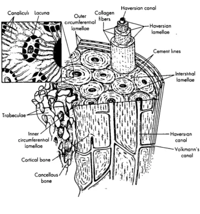
osteon has a central vascular channel with a diameter of 50-90 pm, and this is known as the Haversian canal. It is surrounded by a series of concentric lamellae with osteocytes arranged in a circular pattern. The lamellae spiral around the osteon in layers giving the

secondary osteon a diameter of approximately 200-300 pjm in human bone. The Haversian canal contains blood vessels, nerves, and a variety of cell types depending on the age of the osteon. Osteonal vessels average a diameter of 15 jtm, but grow wider near the endosteal surface. These vessels contain no smooth muscle, but rather are capillaries lined with a layer of endothelial cells. The area between the vessel and canal wall contains a variety of different cells, and it is frequently possible to observe osteoblasts in the process of surrounding themselves with bone matrix. Adjacent to the Haversian canal are the lining cells which are the resting osteoblasts that provide a pool of potential bone-forming cells. [Martin et al. 1989]

2.2.3. Cortical Bone and Trabecular Bone

At the next higher level of bone structure is bone tissue which exists in two fundamental forms: cortical bone and trabecular bone. Cortical bone is a dense material with a specific gravity of approximately 2. It is solid with spaces only for osteocytes, canaliculi, capillaries, or sites of erosion. Cortical bone's smooth outer surface is called the periosteal surface while its internal surface is identified as the endosteal surface.

[Figure 2.8] On the periosteal surface, numerous layers of lamellar bone accumulate forming a thick cortical plate. Trabecular bone, also known as cancellous bone, exists in the metaphyseal region of long bones such as the femur, humerous, radius, ulna, and tibia,

and within the bounds of cortical bone coverings of smaller flat and short bones such as the vertebrae. [Figure 2.9] It is composed of short struts (approximately 0.1 mm in

diameter and extending for about 1 mm) of bone material called trabeculae which can be idealized as rod- and plate-shaped. The connected trabeculae give cancellous bone a spongy appearance; it is quite porous often with half the bone volume associated with pore volume. No blood vessels exist within the trabeculae, but vessels adjacent to the tissue weave in and out of the large spaces between the struts. The material composing trabecular bone is usually primary lamellar bone and sometimes fragments of Haversian bone. In young mammals, it can also be made ofwoven-fibered bone.

The structure of trabecular bone varies both in microscopic and macroscopic anisotropy as well as in its porosity which is proportional to the total volume unoccupied

EPIPHYSIAL REGION

DIAPHYSIAL REGION

EPIPHYSIAL-REGION

ENDOSTEUM

PERIOSTEUM

CANCELLOUS BONE

ICAL BONE

Figure 2.8: Sketch of Longitudinal Section of Femur Illustrating Trabecular and Cortical Bone Types. [Cowin 1981]

by bone tissue. Different variations of the trabeculae pattern are found in characteristically different places. In general the struts with no preferred orientation are found deep in the bone away from loaded surfaces. More oriented struts tend to be observed underneath loaded surfaces where stress patterns are more reasonably constant. Trabecular bone predominates in the epiphyseal region while there is usually very little in the diaphyseal region. As the bone tissue grows on preexisting surfaces, it is often the case that cortical bone is formed in a region where trabecular bone already exists. Where this occurs, the trabecular bone is not replaced, but rather new bone surrounds the preexisting trabeculae

struts resulting in a ambiguous structure pattern with no obvious and distinctive grain.

[Figure 2.10] [Bouvier 1989, Cowin 1986, Currey 1984]

2.2.4. Long Bone Anatomy

The structure of long bone consists of a shaft, known as the diaphysis, with a metaphysis or expansion on each end. [Figure 2.11] In developing, immature bone the metaphysis is surrounded by an epiphysis which is joined to the metaphysis by a

cartilaginous growth plate. The growth plate is where calcification of cartilage takes place, and upon the completion of growth, the epiphysis which is composed of trabecular bone becomes fused with the metaphysis. At the extremity of each epiphysis there is a special covering of articular cartilage which forms a gliding surface for the joint. The coefficient of dry friction between the articular cartilage of the joints can be as low as 0.0026, making the cartilage covering a very effective and efficient joint.

On the outer shell of the metaphyses and epiphyses lies a thin layer of cortical bone that is continuous around the long bone contour and compact around the diaphysis. The diaphysis is basically a hollow tube with walls composed of dense cortical bone that is thick throughout the extent of the shaft. This thickness then tapers off to form the thin shell of the metaphysis. The center space within the diaphysis known as the medullary cavity contains bone marrow. A thin layer of highly active cells which produce circumferential enlargement and remodeling of growing bone is the periosteum which

covers the entire external surface of mature long bone. The outer layer of the periosteum is fibrous and comprises almost the entire periosteum of mature bone, and after maturity,

Haversian canal

Figure 2.10: Schematic Drawing of Shaft of Long Bone Showing Cortical and Trabecular Bone. [Anderson et al 1994]

'Metophlysis

Calci

of cc

Cartilage

-1d1

Development of a long bone

Figure 2.11: (A) Long Bone Anatomy. [Fung 1981]; (B) Development of Long Bone. [Anderson et aL 1994]

this layer of active cells becomes mainly composed of a capillary blood vessel network. In most of the diaphyseal region, the periosteum is thin and loosely attached, and thus the blood vessels are capillary vessels. In contrast, at the expanded ends of the long bone, ligaments are attached firmly and convey larger blood vessels. [Fung 1981]

2.2.5. Remodeling

Studies of cortical and trabecular bone structure have been performed in

conjunction with bone remodeling. Bone remodeling is viewed as a process which adapts bone tissue to the mechanical environment at each point in the structure. In theory, this process optimally adjusts tissue distribution within the bones as a result of the load the bone must bear. The natural remodeling process arranges the given amount of material to support occurring loads with a safety factor.

Living bone is continually undergoing changes of growth, reinforcement, and resorption. This remodeling occurs in two basic ways, external and internal. External remodeling or surface bone remodeling refers to the changes in the shape of the bone caused by movement of external bone surfaces. With increased loads, bone's external surface will move so that the cross-sectional area transverse to the increased load is increased. The reverse will occur with reduced loading. Internal bone remodeling involves changing of the bulk density of bone tissue with stress. When loading applied to the bone is increased, the bulk density of bone tissue will also increase with time. This tissue will also increase stiffness and strength. Conversely, if the loading is decreased, bone tissue density will be reduced as it becomes less strong and less stiff

There are two ways in which concentric cylinders are formed in bone that can be recognized in the formation of the secondary osteon and primary osteon. When the blood vessel is surrounded by preexisting bone, osteoclasts resorb the bone around the blood vessel, and the edges of the cavity are removed while the cement sheath is laid. The cavity then begins to be filled by lamellar bone, and the result is a mature secondary osteon. Here, the course of the preexisting lamellae is interrupted by the osteon. A similar process occurs in the formation of the primary osteon, however, it can only take place on the growing surface. With the primary osteon, the lamellae are uninterrupted by the osteon

and there is no cement sheath. As stated previously, osteons are able to sense direction and gradients of stress. This is evident with observations in the preferred orientation of osteoblasts and osteocytes parallel to collagen fibers, and as remodeling occurs, bone structure is efficiently adapted to changes in mechanical loading and stress-concentrating effects are reduced. [Fung 1981, Currey 1984, Martin et al. 1989]

2.3. Bone Remodeling

The adaptation of trabecular and cortical bone to alterations in their mechanical environment has been of great interest, especially in biomechanics. Reduction in bone density has been observed in periods of disuse in prolonged immobilization. At the same time, increases in bone density have been found in athletes and animals under heavy

exercise. As bone grows in response to the mechanical loading it experiences, evidence of this adaptive phenomenon can be observed in various forms through bone atrophy and hypertrophy. Clinical studies show such evidence in situations such as paralysis and

convalescence during chronic disease states. The exposure of astronauts to weightlessness during space travel has also resulted in a density reduction of the skeletal system. Such findings indicate the response of bone tissue to reduced strain is characterized by a loss of bone tissue mass. Studies have also shown constant peak strain during periods of activity such as exercise.

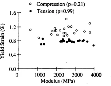
Keaveny et al. (1994) examined the tensile and compressive strengths of bovine tibial trabecular bone and found that strength depends on the density of trabecular bone.

[Figure 2.12] while yield strains were independent of modulus. [Figure 2.13] At the

same time, they determined that the difference between tensile and compressive strengths increases with increasing modulus [Figure 2.14] while the difference between yield strains remains independent of modulus. This conclusion reflects the modulus-dependent

difference between tensile and compressive strengths in trabecular bone and explains some of the seemingly conflicting conclusions drawn on tensile and compressive strengths previously put forth because of variations in the mean modulus. Although Keaveny et

Compression (r2 = 0.66) -- Tension (r2 = 0.66) 0 I I I I I I 0.4 0.5 0.6 Apparent Density 0.7 (gm/cm3)

Figure 2.12: Yield Strength versus Apparent Density for Tensile and Compressive Loading of Bovine Proximal Tibia. [Keaveny et aL 1994]

o Compression (p=0.21) * Tension (p=0.99) oo O 00 0 0 0 00 OD 0 0

AI,,ts.

-a,# I I I 1000 2000 3000 4000 Modulus (MPa)

Figure 2.13: Plot of Yield Strain versus Modulus for Tensile and Compressive Loading of Bovine Proximal Tibia. [Keaveny et aL 1994]

30 - 20- 10-1.6. 1.2- 0.8- 0.4-(1 I 0 f . -I I I I I.v

40 -o - 30_S200 ._ 10-(1 U ' Compression (r2=0.85) *- Tension (r2--0.95) I I I i i I I I 0 1000 2000 3000 4000 Modulus (MPa)

Figure 2.14: Yield Strength versus Modulus for Tensile and Compressive Loading of Bovine Proximal Tibia. [Keaveny et al 1994]

.A

50

loaded in line with principal trabecular orientation, the main stated above conclusions should prove to be valid for most cases of trabecular bone strength.

In general, trabecular bone plays a key role in the function of bone joints since it serves to transmit large contact stresses at the articular surfaces to the cortical bone of the cortical shaft. Through the observations of both trabecular and cortical bone, one can track the morphological changes that bone undergoes in order to accommodate its induced stress requirements.

2.3.1. Historical Remarks

The first attempts to explain trabecular bone structure began in the 19th century when in 1867, G. H. Meyer presented line drawings of the structure he had observed in various bones. He proposed that the spongy material (trabecular bone) in the bone showed a "well motivated architecture which is closely connect with the statics and mechanics of bone." [Roesler 1981] When C. Culmann, a Swiss mathematician, saw Meyer's drawings, he noticed that the lines of the drawings resembled curves of principal

stress trajectories in a crane-like curved bar loaded similarly to that of a human femur. In comparing the drawings of Culmann to his own, Meyer found similarities in the idealized structure of the trabecular bone in the proximal end of the femur and in the Culmann crane. This lead him to believe that the structure oftrabecular bone was influenced by principal stresses.

In 1869, Julius Wolff published his ideas of bone transformation which he

describes as under the influence of "pathological alteration of the external form and under the load on bones, following mathematical rules." [Roesler 1981] In essence he proposed that mechanical stresses affect the remodeling process of bone. Wolff emphasized the idea that the modeling of trabecular bone follows these mathematical rules and later compared the correspondence of the principal stress trajectories of Culmann to the structure of the femur. Both show the crossing at right angles of lines from the drawings and planes from the bone structure that he made at corresponding sections. Wolff's theory became known as the trajectory theory or Wolff's Law. [Figure 2.15] He went on to conclude that

a

Figure 2.15: (a) Frontal Section Through Proximal End Femur, (b) Line Drawing of Trabecular Structure, (c) Culmann's Crane Copied from Wolff. [Roesler 1989]

nature found the most appropriate form and greatest efficiency for bone with minimum material consumption.

W. Roux, in 1885, also proposed a trajectorial architecture of trabecular bone to describe its geometry to explain how its organization provides maximum strength with a minimum amount of material. These same ideas were also echoed by F. Pauwels (1948) who conducted photoelastic experiments toward this theory, and J.C. Koch (1917) who performed detailed strength of materials analysis of the human femur and the architecture of trabecular bone within it. Koch concluded that trabeculae in the proximal femur were arranged in tensile and compressive systems aligned in the principal stress directions while the spacing and thickness of the trabeculae vary with stress magnitudes. [Hayes et al.

1981]

2.4. Experiments and Morphological Changes

When attempting to verify the validity of the concepts established by Wolffs Law, experiments on bone tissue are executed to evaluate the influence of loading history alterations on bone remodeling. The response of bone can be generalized as the arrangement of a new bone matrix and/or the resorption of existing bone. As a result

common ways to assess the remodeling of bone tissue are to look at the effect of bone atrophy and hypertrophy. Most of the experiments that have been performed looked at the changes of cortical bone and trabecular bone density with changing load.

2.4.1. Bone Remodeling: Assumptions

When attempting to predict and understand the response of bone to changes in mechanical load, it is important to understand the way the changes are sensed in the bone itself. Alterations in bone function are induced by changes in loading and loading pattern. If bone remodeling is to be considered site specific, a local and physically measurable display of the modified loading must exist at varying points in bone.

For Hookean materials, mechanical stress and strain are often used interchangeably since they are proportional. Bone is linear elastic, but its modulus depends on morphology

because it is a nonhomogeneous, anisotropic material. Through results in many in vivo strain gauge experiments, it has been concluded that bone senses change in functional use by measuring strain. This conclusion is reinforced with the finding of nearly constant peak functional strains of bones with the same function in a wide variety of animals and by Keaveny et al. 's. finding of a constant strain to failure in trabecular bone.

Experiments have shown that the peak strain at functionally equivalent sites in growing bone are constant throughout the growth period. Regardless of bone size and activity in each of the different species, peak functional strains in the bones of different animals with similar function were all within the range of 2000-3000

w.

as can be seen in Table 2.1. In contrast, evidence shows that peak stresses in bone during various activities differ greatly in different animals and are correlated with body mass. Thus it seems that strain equilibrium is achieved by adaptive response. Strain history, being the probably mechanical source that regulates the adaptive response of bone, embodies all past strain variations such as:

* Magnitude

* Strain Mode (tension, compression shear in a particular plane) * Strain Rate (bone deformation rate)

* Strain Frequency (deformation cycles per second)

* Stimulus Duration (total number of deformation cycles or time over cycles applied) * Strain Distribution (pattern of strain magnitude across bone section)

* Strain Energy (elastic energy stored or dissipated during deformation) * Strain Direction (principal strain direction relative to bone surface)

Looking at the data from Keaveny et al., the authors show that the trabecular bone of the bovine proximal tibia achieves a compressive yield strain of approximately 1.0% while the tensile yield strain reaches approximately 0.8%. [Figure 2.13] S.C. Cowin (1989) also reports for cortical bone tissue of bovine femoral bone an average compressive yield strain in the axial direction of 2.53% and an average axial tensile yield strain of 3.24%.

Comparing these data and with the peak compressive functional strains of 0.2-0.3%, we can see that trabecular and cortical bone maintain a safety factor of 4 and 10, respectively, inherent in their remodeling so as to prevent failure.

Table 2.1: Peak Functional strains in animals. [Martin et al. 1989]

Bone Activity Peak Strain

Horse radius Trotting -2800

Horse tibia Galloping -3200

Horse metacarpal Acceleration -3000

Dog radius Trotting -2400

Dog tibia Galloping -2100

Goose humerus Flying -2800

Cockerel ulna Flapping -2100

Sheep femur Trotting -2200

Sheep humerus Trotting -2200

Sheep radius Galloping -2300

Sheep tibia Trotting -2100

Pig radius Trotting -2400

Fish Hypural Swimming -3000

Macaca mandible Biting -2200

Another assumption to take into account when considering remodeling is the concept of a steady-state range. This remodeling equilibrium can be characterized as the bone loading situation where bone tissue is being simultaneously resorbed and deposited while maintaining no net change in its macroscopic properties or geometry. Because bone functions cover a wide spectrum of activities, it is likely that the strain values that

compose equilibrium are site specific and bone specific. Remodeling equilibrium can also be changed due to processes such as aging or changes in hormonal, genetic, and metabolic

activity. These changes usually introduce complexity in remodeling theories concerned with mechanical adaptation processes and are usually assumed constant during net

remodeling behavior where mechanical input is the chief stimulus.

Since it has been established that strain is the mechanical parameter that is sensed, the question now remains as to the mechanism by which strain influences the remodeling process. There have been several proposed mechanisms which include diffusion effects

and damage accumulation. One hypothesis is that material strains directly affect osteocyte (bone-maintaining cells) cell membranes or their extracellular components. Another possible mechanism for bone remodeling in cancellous bone is the continuous repair of microfractures in the trabeculae. Experiments performed on rabbit tibia subject to intermittent loading showed microfractures with greater disorganization and greater remodeling activity as well as significant stiffening of the trabeculae. It can be said that the trabecular bone acts as a shock absorber with microfractures as the mechanism for energy absorption, and subsequently the microfractures remodel into stronger tissue that is more dense. It is likely that a combination of these effects and others influence the

remodeling of trabecular bone. [Cheal 1986, Martin et al. 1989, Hart et al. 1989]

2.4.2. Experiments: Bone Atrophy

Evidence that is most often cited as an indicator of the effect of mechanical loading on bone from regulation is bone atrophy where normal functioning loads are eliminated. This condition is known as disuse osteoporosis, or more accurately, osteopenia.

Assuming an equilibrium point between tissue deposition and resorption mediated by some mechanical forces (and several other biological factors which also come into play), atrophy

due to a drastic reduction in mechanical forces leads to decreased bone mass. Bone atrophy also encompasses the effects of noncatastrophic, long term decreases in strain experienced by bone which were previously uninvestigated have become of great intrigue. Long term success of an implant is dependent on its compatibility. In the case of hip

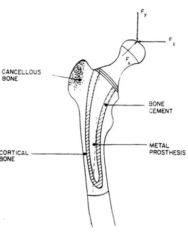
implants, a decreased stress is experienced in the proximal end of the femur because the load is transmitted through the implant stem to the midshaft. [Figure 2.16] As a result, bone resorption may occur because of the reduced loading experienced and cause a

subsequent loosening of hip implants. From this example, one can see the alterations of stress influence the stress distribution around the implants, and this has been one of the motivating factors to better characterize the relationship between loading history and bone remodeling.

Immobilization studies are the most effective in providing insight to the effects of decreased loading. Some of the first studies done on bone atrophy by Allison and Brooks (1921) on dogs, by Geiser and Treuta (1958) on rabbits, and by Kazarian and Von Gierke (1961) on monkeys note a loss of trabecular tissue when load reductions were imposed on various bones. In the case of Kazarian and Von Gierke, bone loss was characterized as a decrease in the number and thickness of trabeculae as the adult monkeys were subjected to total body casting. At the same time cortical volume was also decreased as its thickness was reduced 15%. [Meade 1989]

More recent studies were done by Uhthoff et al. (1978) and Jaworski et al. (1980) who examined long term immobilization effects on young and old beagle dogs. These studies showed the responses of animals of different age groups when experiencing a change in load history. The initial bone volume of the young adult dogs (weighing 7-13

kg) and the older adult dogs (age 7-8, weighing 11-16 kg) is expressed as the ratio of

cortical bone area to the total area of the cross-section at mid-diaphysis. As shown in

Table 2.2, there was a 5-12% reduction in initial bone volume of the older dogs compared

to the younger. Forelimbs of both dogs were immobilized by a plaster cast and then sacrificed between 2-40 weeks after initiation. The experimental animals showed decrease in bone density and increase in medullary canal after 32-40 weeks while the outside

CANCELLC BONE L THESIS CORTICAL BONE

Figure 2.16: Femoral Component of Total Hip Replacement and Applied Joint Force Components. [Cowin 1989]

Table 2.2: Bone Volume as Cortical Bone Area to Total Area of Cross-Section of Four Bones in Young Adult and Older Beagle Dogs Before Immobilization. [Jaworski et al. 1980]

Male Female

Bone Young Old % Difference Young Old % Difference

Third Metacarpal 86± 0.9 79± 2.9 8.14 86± 0.5 80± 0.5 6.98

Ulna 80+ 0.5 75+ 1.2 6.25 80+ 0.8 76+ 1.4 5.00

Radius 80± 1.3 71± 2.0 11.25 81±0.7 75+ 1.0 7.41

Humerus 68±2.2 63± 1.1 7.35 70± 2.9 62 2 0 11.43

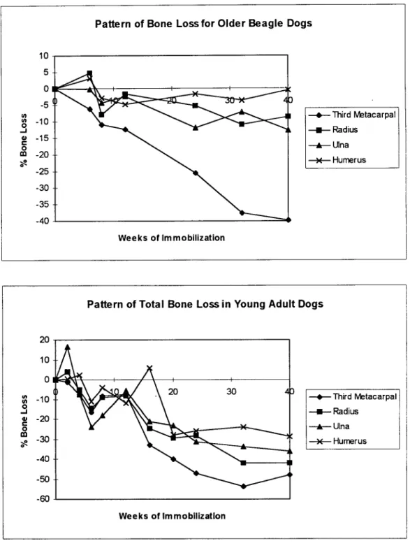
reduction on the periosteal envelope in the younger dogs. Cross-sectional measurements were taken at 40 weeks of the mid-diaphysis of the third metacarpal, radius, ulna, and humerus [Figure 2.17] showing a reduction in cortical bone thickness due to expansion of the medullary cavity. The pattern of bone loss was studied with respect to the duration of immobilization. Their findings were consistent with others showing trabecular bone loss at mid-diaphysis of the immobilization bone, however, losses fluctuated throughout the experiment without any development of a discernible pattern. [Figure 2.18] Tables

2.3-2.6 show the histomorphometric details of the aforementioned bones for the older dogs

while Tables 2.7-2.10 reveal the results of the young adult dogs for each of these bones. At the end of bone experiments, the greatest bone loss was experienced in the third metacarpal and the least in the humerus.

The pattern of bone loss for the young adult and older dogs is characterized in three stages: rapid bone loss followed by reversal, gradual and more sustained bone loss, and stabilization of bone loss. Although the older dogs began the experiment with less bone mass than the younger dogs, they seemed to lose less bone during the 40-week experimental period while their stages of bone loss appeared less distinct. Another interesting observation was that the periosteal envelope contributed to most of the bone loss in younger dogs while the endosteal surface did so for the older dogs. The

differences in the behavior of these bone envelopes which encase the cortex of the diaphysis seem to vary more than trabecular bone which only has one surface, the

Figure 2.17: Cross-section of Third Metacarpal at 40 weeks. (Top) Control; (Bottom) Experimental Side Showing Expansion of Medullary Cavity and Thinning of Cortex. Scale is in millimeters.

[Jaworski et al. 1980]

Pattern of Bone Loss for Older Beagle Dogs

Figure 2.18: Graph Relating Bone Loss Pattern to Immobilization Duration Expressed as Percentage of Control. [Jaworski et al. 1980, Uhthoff et al. 1978]

lU 5 0 -5 , -10 * -15 m -20 -25 -30 -35 -40 T-- hird Metacarpal -u- Radius --- Ulna -- Humerus Weeks of Immobilization -40

Table 2.3: Histomorphic Data for Third Metacarpal of Old Beagle Dog [Jaworski et aL 1980]

Tot Cross-Sectional Area (mm^2) Medullary Canal Area (mm^2) Area of Porosity (mm^2) Total Weeks Experi- Experi- Difference Expen- Difference Percent in Cast mental Control mental Control mmA2 % mental Control mmA2 % Difference

6 13.25 13.00 2.25 1.50 -0.75 -654 0.27 0.05 -0.22 -1.92 -6.28 8 15.61 16.23 3.21 3.13 -0.08 -0.61 0.82 0.08 -0.74 -5.68 -11.05 12 19.60 19.60 4.57 3.41 -1.16 -7.30 1.09 0.29 -0.80 -5.03 -12.33 24 14.10 14.93 3.81 1.58 -2.23 -16.73 0.36 0.02 -0.34 -2.55 -25.51 32 15.07 16.60 6.96 4.20 -2.76 -22.64 0.51 0.21 -0.30 -2.46 -37.65 40 18.88 18.73 8.86 2.69 -6.17 -37.15 0.54 0.28 -0.26 -1.65 -39.85

Table 2.4: Histomorphic Data for Radius of Old Beagle Dog [Jaworski et aL 1980]

Tot Cross-Sectional Area (mm^2) Medullary Canal Area (mm^2) Area of Porosity (mm^2) Total Weeks Experi- Experi- Difference Experi- Difference Percent

in Cast mental Control mental Control mm^2 % mental Control mm^2 % Difference

6 31.75 30.38 5.88 5.63 -0.25 -1.02 0.08 0.16 +0.08 +0.33 +4.88 8 39.34 41.71 9.54 9.59 +0.05 +0.16 0.38 0.21 -0 17 -0.53 -7.83 12 56 30 56.70 13.80 14.30 +0.50 +1.20 1.58 0.74 -0.84 -2.02 -1.78 24 42.06 42.78 11.19 10.29 -090 -2.78 0.11 0.06 -0.05 -0.15 -5.15 32 45.39 47.03 12.70 10.50 -2.20 -6.05 0.28 0.12 -0.16 -0.44 -11.00 40 48.67 50.08 12.50 11.25 -1.25 -3.29 1.41 0.82 -0.59 -1.55 -8.55

Table 2.5: Histomorphic Data for Ulna of Old Beagle Dog [Jaworski et aL 1980]

Tot Cross-Sectional Area (mm^2) Medullary Canal Area (mm^2) Area of Porosity (mmA2) Total Weeks Experi- Experi- Difference Experi- Difference Percent

in Cast mental Control mental Control mmA2 % mental Control mmA2 % Difference

6 30.13 28.00 6.38 4.00 -2.38 -9.86 0.08 0.26 +0.18 +0.75 -0.29 8 33.07 34.19 7.04 7.38 +0.34 +1.29 0.75 0.39 -0.36 -1.36 -4.31 12 51.70 51.30 12.33 11.50 -0.83 -2.20 1 68 1.22 -0.46 -1.22 -2.36 24 30.06 33.38 6.07 6.07 0 0 0 09 0.16 +0.07 +0.26 -11.97 32 44.09 44.04 11.73 9.76 -1.97 -5.84 1.02 0.53 -0.49 -1.45 -7.14 40 42.17 47.42 9.00 10.17 +1.17 +3.22 1.39 0.92 -0.47 -1.29 -12.56

Table 2.6: Histomorphic Data for Humerus of Old Beagle Dog [Jaworski et aL 1980]

Tot Cross-Sectional Area (mm^2) Medullary Canal Area (mm^2) Area of Porosity (mm^2) Total Weeks Experi- Experi- Difference Experi- Difference Percent in Cast mental Control mental Control mm^2 % mental Control mm^2 % Difference

6 72.00 70.50 22.25 22.25 0 0 0.18 0.17 -0.01 -0.02 +3.10 8 91.69 92.07 38.25 37.44 -0.81 -1.50 0.82 0.51 -0.31 -0.57 -2.77 12 116.00 114.00 44.20 39.40 -4.80 -6.45 0.83 0.76 -0.07 -0.09 -4.66 24 82.11 85.14 27.29 30.09 +2.80 +5.13 1.22 0.48 -0.74 -1.36 -1.78 32 89.50 88.40 31.20 28.10 -3.10 -5.21 0.89 0.81 -0.08 -0.13 -3.49 40 106.70 106.90 36.50 36.63 +0.13 +0.19 1.49 1.19 -0.30 -0.43 -0.53

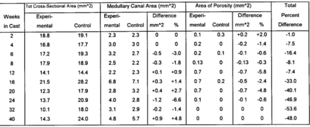
Table 2.7: Histomorphic Data for Third Metacarpal of Young Beagle Dog [Uhthoff et al. 19781

Tot Cross-Sectional Area (mm^2) Medullary Canal Area (mm^2) Area of Porosity (mm^2) Total Weeks Experi- Experi- Difference Experi- Difference Percent

in Cast mental Control mental Control mm^2 % mental Control mmA2 % Difference 2 18.8 19.1 2.3 2.3 0 0 0.1 0.3 +0.2 +2.0 -1.0 4 16.8 17.7 3.0 3 0 0 0 0.2 0 -0.2 -1.4 -7.5 6 17.2 19.3 3.2 2.7 -0.5 -3.0 0.2 0.1 -0.1 -0.6 -16.4 8 17.9 18.9 2.5 2.2 -0.3 -1.8 0.13 0 -0.13 -0.3 -8.1 12 14.1 14.4 2.2 2.3 +0.1 +0.9 0.7 0 -0.7 -5.8 -7.4 16 21.5 28.2 6.8 7.1 +0.3 +1.4 07 0.2 -0.5 -2.4 -33.0 20 12.3 17.9 2.8 3.2 +0.4 +2.7 0.7 0 -0.7 -4.8 -40.1 24 13.7 20.9 4.0 2.8 -1.2 -6.6 0.1 0 -0 1 -0.6 -46.9 32 10.1 18.0 3.1 2.9 -0.2 -1.4 0 0 0 0 -53.6 40 14.3 24.0 4.8 5.7 +0.9 +4.8 0 0 0 0 -48.0

Table 2.8: Histomorphic Data for Radius of Young Beagle Dog [Uhthoff et aL 1978]

Tot Cross-Sectional Area (mm^2) Medullary Canal Area (mm^2) Area of Porosity (mm^2) Total

Weeks Experi- Experi- Difference Experi- Difference Percent in Cast mental Control mental Control mm12 % mental Control mm^2 % Difference

2 53.0 50.0 13.5 11.9 -1.6 -4.3 0.2 0.3 +0 1 +0.3 +4.0 4 49.5 52.0 8.6 10.2 +1.6 +3.9 1.3 0.1 -1 2 -2.9 -5.0 6 48.3 50.8 12.8 0.3 -12.5 -8.4 0 0 0 0 -14.5 8 540 56.3 13.3 11.7 -1.6 -3.6 0.2 0 -0.2 -0.4 -9.1 12 41.7 42.9 9.8 8.5 -1.3 -3 8 0.4 0 -0.4 -1.0 -8 4 16 103.5 121.8 42.2 42.9 +0.7 +0.8 2.3 0.7 -1.6 -2.0 -24.6 20 49.4 57.8 20.0 16.2 -3.8 -9.1 0.1 0.1 0 0 -29.4 24 50.7 54.5 19.9 11.6 -8.3 -19.3 0 0 0 0 -28.2 32 35.2 55.1 11.2 13.7 +2.5 +6.0 0 0 0 0 -42.0 40 59.8 77.4 29.2 24.8 -4.4 -8.4 0.2 0.3 +0.1 +0.2 -41.9

Table 2.9: Histomorphic Data for Ulna of Young Beagle Dog [Uhthoff et aL 1978]

Tot Cross-Sectional Area (mm^2) Medullary Canal Area (mm^2) Area of Porosity (mm^2) Total Weeks Expern- Experi- Difference Experl- Difference Percent in Cast mental Control mental Control mm^2 % mental Control mmA2 % Difference

2 39.9 32.9 9.6 6.7 -2.9 -11.3 0.5 0.6 +0.1 +0.4 +16.4 4 32.8 34.4 6.4 6.6 +0.2 +0.7 0.7 0.1 -0.6 -2.2 -7.3 6 31.0 36.7 8.3 7.0 -1.3 -4.5 0.3 0.3 0 0 -24.1 8 41.6 49.0 9.3 9.5 +0.2 +0.5 0.1 0.4 +0.3 +0.3 -18.1 12 29.2 32.0 6.2 7.0 +0.8 +2.0 0.2 0 -0.2 -0.5 -5 6 16 87.5 115.2 27.8 40.2 +12.4 +168 1.4 1.2 -0.2 -0.3 -21.0 20 41.4 40.8 16.3 8.4 -7.9 -24.6 0.3 0.2 -0.1 -0.3 -23.0 24 38.2 46.2 12.9 9.6 -3.3 -9.1 0.1 0 -0.1 -0.3 -31.3 32 32.8 41.7 10.3 7.6 -2.7 -7.9 0 0.1 +0.1 +0.3 -33.8 40 43.8 54.1 16.0 11.2 -4.8 -11.3 0.6 0.3 -0.3 -0.7 -36.2

Table 2.10: Histomorphic Data for Humerus of Young Beagle Dog [Uhthoff et aL 1978]

Tot Cross-Sectional Area (mrn2) Medullary Canal Area (mm^2) Area of Porosity (mm^2) Total Weeks Experi- Experi- Difference Experi- Difference Percent in Cast mental Control mental Control mm^2 % mental Control mm^2 % Difference

2 91.1 92.9 30.1 31.1 +1.0 +2.0 0.6 0.7 +0.1 +0.2 +0.2 4 106.8 101.6 40.2 36.6 -3.6 -5.6 0 0 0 0 +25 6 98.4 105.0 35.4 34.6 -0.8 -1.1 0.3 0.1 -0.2 -0.3 -10.8 8 97.8 201.8 32.8 33.3 +0.5 +0.7 0 0 0 0 -3.8 12 83.2 85.9 32.2 28.3 -3.9 -6.8 0.1 0 -0.1 -0.2 -11.7 16 203.1 205.1 105.8 102.1 -3.7 -3.6 0.5 02 -0.3 -0.3 +5.8 20 100.3 105.3 51.2 37.1 -14.1 -20.7 0.7 0.13 +0.6 +0.1 -27.9 24 105.6 129.1 46.2 48.8 +2.6 +3 2 0 0 0 0 -26.0 32 92.9 105.9 41.5 38.4 -3.1 -4.6 0.13 0.17 +0.04 0 -23.9 40 141.7 157.9 81.6 73.6 -8.0 -9.5 0.37 0.38 +0.01 0 -28.8