The 6D bias and the equity premium puzzle

Digitized

by

the

Internet

Archive

in

2011

with

funding

from

Boston

Library

Consortium

IVIember

Libraries

'IB31

!,M15

)

DEWEY

01

Massachusetts

Institute

of

Technology

Department

of

Economics

Working

Paper

Series

THE

6D

BIAS

AND

THE

EQUITY

PREMIUM

PUZZLE

Xavier

Gabaix

David

Laibson

Working

Paper

02-01

Jurie

2001

Room

E52-251

50

Memorial

Drive

Cambridge,

MA

021

42

This

paper

can be downloaded

without

charge from

the

Social

Science

Research Network

Paper

Collection at

\V'

Massachusetts

Institute

of

Technology

Department

of

Economics

Working Paper

Series

THE

6DBIAS

AND

THE

EQUITY

PREMIUM

PUZZLE

Xavier

Gabaix

David Laibson

Working

Paper

02-01

June

2001

Room

E52-251

50

Memorial

Drive

Cambridge,

MA

021

42

This

paper can be

downloaded

without

charge from

the

Social Science

Research Network

Paper

Collection at

The

6D

bias

and

the equity

premium

puzzle

Xavier

Gabaix

David

Laibson

MIT

Harvard

University

and

NBER*

Current

Draft:

June

24,

2001

First Draft:

August

15,

2000

Abstract

Ifdecision costs lead agents to update consumption every

D

periods, then econometricians

willfindan anomalously lowcorrelationbetweenequity returnsandconsumptiongrowth (Lynch

1996).

We

analytically characterize the dynamic properties of an economy composed of

con-sumers

who

have such delayed updating. In our setting, an econometrician using an Euler

equation procedure would infer a coefBcient ofrelative risk aversion biased up by a factor of

6D. Hence with quarterly data, ifagents adjust their consumption every

D

=

4 quarters, the imputed coefficientofrelative risk aversion willbe 24 times greater than the truevalue. High

levelsofrisk aversion impliedbythe equity

premium

andviolationsofthe Hansen-Jagannathan boundsceasetobe puzzles.

The

neoclassical modelwith delayed adjustment explainsthe

con-sumption behaviorof shareholders. Oncelimitedparticipationistakenintoaccount, themodel

matches mostproperties ofaggregate consumptionand equityreturns, including

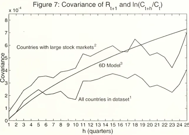
new

evidence

thatthe covariancebetween \n{Ct+h/Ct) and Rt+i slowlyriseswith h.

Keywords:

61?,

bounded

rationality, decisioncosts, delayed adjustment, equity

premimn

puzzle

JEL

classification:

E44

(financial markets

and

the

macroeconomy),

Gl

(general financial

mar-kets).

'Gabaix:DepartmentofEconomics,

MIT,

Cambridge,

MA

02142,xgabaix@mit.edu. Laibson:Department

ofEconomics, HarvardUniversity, and

NBER,

Cambridge

MA

02138, dlaibson@harvard.edu.

We

thankBen

Bernanke, Olivier Blanchard, John Campbell, James Choi, Karen Dynan, George Constantinides, John

Heaton, Robert Lucas, Anthony Lynch, Greg Mankiw, Jonathan Parker, Monika Piazzesi,

Ken

Rogoff,

James Stock,

Jaume

Ventura, Annette Vissing, and seminar participants at Delta, Insead, Harvard, MIT, University of Michigan,

NBER,

and

NYU

for helpful comments.

We

thank Emir Kamenica, Guillermo

Moloche, Eddie Nikolovaand Rebecca Thorntonfor outstandingresearcheissistance.

iMSSACHUSEnsTNS

111UTE OFTEGHMntOGY

WAR

7

2002

1

Introduction

Consumption

growth covaries only weakly with equity returns, which implies that equities are not very risky. However, investors havehistoricallyreceived avery large

premium

for holdingequities.

For twenty years, economists have asked

why

an asset with little apparent risk has such a large

required return.'

Grossman

and Laroque

(1990) argued thatadjustment costs might answer the equity

premium

puzzle. If it is costly to change consumption, households will not respond instantaneously to

changes in asset prices. Instead,

consumption

will adjust with a lag, explaining

why

consumption

growth covariesonlyweakly withcurrent equityreturns. In the

Grossman

and Laroque

framework, equities are risky, but that riskiness does not

show

up

in a high

contemporaneous

correlation

between consumption growth

and

equity returns.

The comovement

is only observable in the long-run.

Lynch

(1996)

and

Marshall

and Par«kh

(1999)have simulateddiscrete-timedelayedadjustments models

and

demonstrated that these models can potentially explain the equity

premium

puzzle.^

In light ofthe complexity ofthese models, both sets ofauthors used numerical simulations.

We

propose a continuous-timegeneralization ofLynch's (1996) model.

Our

extension provides

two

new

sets of results. First, our analysis is analytically tractable;

we

derive a complete

ana-lytic characterization of the model's

dynamic

properties. Second, our continuous-time

framework

generates effects that are

up

tosix times larger than those in discrete time models.

We

analyze an

economy

composed

ofconsumers

who

update

their

consumption

every

D

(as

in Delay) periods.

Such

delays

may

be

motivated

by

decision costs, attention allocation costs, and/or mental accounts.^

The

core ofthe paper describes the consequences of such delays. In

addition,

we

derive a sensible value of

D

based on a decision cost framework.

The

"61? bias" is our key result. Using datafrom oiu: economy, an econometrician estimating thecoefficientofrelative riskaversion

(CRRA)

fromthe

consumption

Euler equation

would

generate

a multiplicative

CRRA

bias of

6D.

For example, if agents adjust their

consumption

every Z)

=

4

quarters,

and

the econometrician uses quarterly aggregates in his analysis, the

imputed

coefficient of relative risk aversion will

be

24 times greater than the true value.

Once we

take account of

this

6D

bias, theEuler equationtests areunableto reject the standard

consumption

model.

High

equity returns

and

associated violations of the

Hansen-Jagannathan

(1991)

bounds

cease to

be

puzzles.

The

basic intuition for this result is quite simple. If households adjust their

consmnption

every

D

>

1 periods, then

on

average only

_^

households will adjust each period. Consider only

the households that adjust during the current period

and assume

that these households adjust

consumption

at dates spread uniformly over the period. Normalize the timing so the current

period is the timeinterval [0, 1].

When

a household adjusts at time i

G

[0,1], it can only respond

toequity returns that havealready

been

realized

by

timei. Hence, thehouseholdcanonly respond

to firaction i ofwithin-period equity returns. Moreover, the household that adjusts at time i can

only change

consumption

for the remainder of the period. Hence, only fraction (1

—

i) of this

'For theintellectualhistoryof thispuzzle,seeRubinstein(1976), Lucas(1978),Shiller(1982), Hansen and Single-ton (1983), Mehraand Prescott (1985), and Hansen and Jagannathan (1991). Foruseful reviews see Kocherlakota

(1996)and Campbell (2000).

-See also related work by Caballero (1995), He and Modest (1999), Heaton and Lucas (1996), Luttmer (1995),

and Lynch and Balduzzi (1999).

See Gabaix and Laibson (2000b) for a discussion ofdecision costs and attention allocation costs. SeeThaler

period's

consumption

is affected

by

the change at time i.

On

averagethe households that adjust

during the current period display a covariance

between

equity returns

and consumption growth

that isbiased

down

by

factor

/I

1

/ t{l -i)di

=

-.

The

integral is taken from to 1 to average over the uniformly distributed adjustment times.

Since only fraction -^ ofhouseholds adjust in thefirst place, the aggregate covariance

between

equityretiu-ns

and consumption growth

isapproximately_g--^ as large asit

would be

ifallhouseholds

adjusted instantaneously.

The

Eulerequationforthe instantaneous adjustment

model

impliesthat

the coefficient of relative risk aversion isinverselyrelated to the covariance

between

equity returns

and consumption

growth. If

an

econometrician used this Euler equationto

impute

the coefficient of relative risk aversion,

and

he used data

from

our delayedadjustment economy, he

would impute

a coefficient ofrelative risk aversion that

was

6D

times too large.

In section 2

we

describe our formal model, motivate our assumptions,

and

present our key

analjrtic finding. In section 2.2

we

provide

an

heuristic proofof our results for the case

D

>

1.

In section 3

we

present additional results that characterize the

dynamic

properties of our

model

economy. In section 4

we

close our

framework by

describing

how

D

is chosen. In section 5

we

consider the consequences ofour

model

for

macroeconomics

and

finance. In section 6

we

discuss

empirical evidence that supports the

Lynch

(1996)

model and

our generalization.

The

model

matches

most

ofthe empirical

moments

of aggregate

consumption

and

equity returns, including a

new

test

which

confirms the

6D

prediction that the covariance

between

\n{Ct+h/Ct)

and

Rt+i shouldslowly rise with h. In section 7

we

conclude.

2

Model

and

key

result

Our

framework

is a synthesis of ideas

from

the continuous-time

model

of

Merton

(1969)

and

the

discrete-time

model

of

Lynch

(1996). In essence

we

adopt Merton's continuous-time modeling

approach

and

Lynch's emphasis

on

delayedadjustment.^

We

assume

that the

economy

has

two

linear production technologies: a risk free technology

and

arisky technology (i.e., equities).

The

risk free technology has instantaneous return r.

The

returns from the risky technology follow a geometric diffusion process with expected return r

+

tt

and

standarddeviation a.

We

assume

that

consumers

hold

two

accounts: achecking account

and

abalanced

mutual

fund.

A

consumer's checking account is used for

day

to

day

consumption,

and

this account holds only

the risk free asset.

The

mutual

fundis used to replenish the checking account

from

time to time.

The

mutual

fund is professionally

managed

and

is continuously rebalanced so that d share of the

mutual

fund assets are always invested in the risky asset.^

The

consumer

is able to pick 9.^ In

practice, the

consumer

picks a

mutual

fund that maintainsthe consumer's prefered value of6.

We

call6 the equity share (in the

mutual

fund).

Every

D

periods, the

consumer

looks at her

mutual

fund

and

decides

how much

wealth to

withdraw

from the

mutual

fund to deposit in her checking account.

Between

withdrawal periods

—

i.e., from withdrawal date t to the next withdrawal date t

+

D

—

the

consumer

spends

from

SeeCalvo(1983), Fischer (1977),andTaylor(1979)forearlierexamplesofdelayedadjustmentinmacroeconomics. This assumption can be relaxed without significantly changing the quantitative results. In particular, the

her checking account

and

does not monitor her

mutual

fund. For

now we

take

D

to be exogenous.

Following aconceptual approach takeninDuffie

and Sun

(1990),

we

latercalibrate

D

witha decision

cost

model

(see section 4). Alternatively,

D

can be motivated with a mental accounting

model

of

the type proposed by Thaler (1992).

Finally,

we

assume

that consumers have isoelastic preferences

and

exponential discount

func-tions:

Uu

=

Et

r

e-f^^~'^ _{

n^-^

)

^^-Here i indexes the individual

consumer

and

t indexes time.

We

adopt the following notation. Let Wit represent the wealth in the

mutual

fund at date t.

Between

withdrawaldates,

wn

evolves according to

dwit

=

Wit ((^

+

0'K)dt

+

Oadzt),

where

2j is a

Wiener

process.

We

can

now

characterize the optimal choices ofour consumer.

We

describe each date at which the

consumer

monitors

—

and

in equilibrium

withdraws

from

—

her

mutual

fund as a "reset date." Formalproofs of allresults are provided in the appendix.

Proposition

1

On

the equilibrium path, thefollowing properties hold.

1.

Between

reset dates, consumption grows at afixed rate -{r

—

p).

2.

The

balance in the checking account just after a reset date equals the net present value of

consumption between reset dates, where the

NPV

is taken with the risk free rate.

3.

At

reset date t, consumption is 0,,.+

=

aw^T—, where

a

is a function ofthe technology

para-meters, preference parapara-meters,

and

D.

4-

The

equity share in the mutual

fund

is

Note

that 0^^.+ represents consumption immediately after reset

and

w^t- represents wealth in

the

mutual

fund immediately beforereset.

Claim

1follows fromthepropertythat

between

resetdatesthe rate of return tomarginalsavings

is fixed

and

equal to r.

So

between reset dates the

consumption

path grows at the rate derived in

Ramsey's

(1928) original deterministic growth model:

-

=

-(''-P)-c

7

Claim

2 reflects the advantages of holding wealth in the balanced

mutual

fund. Instantaneous

rebalancing of this fund

makes

it optimal to store 'extra' wealth

—

i.e., wealth that isnot needed

for

consumption between

now

and

the next reset date

—

in the

mutual

fund.

So

the checking

account is exhausted between reset dates.

Claim

3 follows from the homotheticity ofpreferences.

Claim

4

imphes

that the equity share is equal to the

same

equity share derived

by

Merton

(1969)

in his instantaneous adjustment model. This exact equivalence is special to our institutional

(see Rogers 2001 for numerical examples in a related model).

Note

that the equity share is

increasing in the equity

premium

(vr)

and

decreasing in the coefficient of relative risk aversion ₍₇₎

and

the variance of equity returns (cr^).

Combining

claims 1-3 results

imphes

that the optimal

consumption path between

date

r and

date

T

+

D

is Cit

=

ae~i ' _w^^-

and

_{the optimal balance in the checking} account _{just after}

reset date r is

T+D

Cis^ ^(^-^)(is

=

/T

+

D

l^r-p)is-r)-ris-r)^

Claim

3 implies that at reset dates optimal

consumption

is linear in wealth.

The

actual value

of the propensity to consume, a, does not matter for the results that follow.

Any

linear rule

—

e.g., Hnear rules of

thumb

—

will suffice. In practice, theoptimal value of

a

in our

model

will

be

close to theoptimal marginal propensity to

consume

derived

by

Merton,

a

=

^+fl-i

r

+

7

\^

77

_V 27CT^^

Merton's value is exactly optimal in our

framework

when

D

=

0.

2.1

Our

key

result:

the

6D

bias

In our economy, each agentresets

consumption

at intervals of

D

units of time. Agents are indexed

by

their reset time i

G

[0,D).

Agent

i resets

consumption

at dates {i,i

+

D,i

+

2D,

...}.

We

assume

that the

consumption

reset times are distributed uniformly.*^

More

formally, there

exists a

continuum

ofconsumers

whose

reset indexes i aredistributeduniformlyover [0,D). Sothe

proportion ofagents resetting their

consumption

in any time interval oflength

At

<

D

is

At/D.

To

fixideas, supposethatthe unit oftimeisa quarterofthecalendaryear,

and

D

—

4. In other

words, thespan oftime

from

^ to t

+

1 is one quarter ofayear. Since

D

=

4, each

consumer

will

adjust her

consumption

once every four quarters.

We

will often choose the slightly non-intuitive

normalization that a quarter ofthe calendar year is one period, since quarterly dataisthe natural

unit oftemporal aggregation with

contemporary

macroeconomic

data.

Call Ct the aggregate

consumption between

t

—

1

and

t.

Ct

Ji=0 LJs=t-l

Cisds

ld^.

Note

that

jg:^i_i(ksds is per-period

consumption

for

consumer

i.

Suppose

that an econometrician estimates

_{7 and}

_f3 using a

consumption

Euler equation (i.e.,

the

consumption

CAPM). What

will the econometrician inferabout preferences?

Theorem

2 Consider

an

economy

with true coefficient of relative risk aversion 7. econometrician estimates the Euler equation

Suppose

an

Et-i

P

Ct Ct-i

—

r

m

1

for two assets, the risk free bond

and

the stock market. In other words, the

econometncian

fits {3

and

7

to

match

the Euler equation above for both assets.

Then

the econometrician willfind

r6D7

for

D>1

^'\

3(T3^H^7

for

0<D<1

^'^

plus higher order terms characterized in subsequent sections.

Figure 1 plots

_7/7

as a function ofD.

The

formulae for the cases

<

Z?

<

1

and

D

>

1 are taken

from

Theorem

2.

Insert Figure 1 about here

The

two

formulae paste at the crossover point,

D

=

1. Convexity of the formula below

D

=

1,

implies that

_7/7

> 6D

for all values of

D.

The

case of instantaneous adjustment (i.e.,

D

=

0)

is of

immediate

interestsince it has been solved already

by

Grossman,

Melino,

and

Shiller (1987).

With

D

=

the only bias arises from time aggregation ofthe econometrician's data, not delayed

adjustment by consumers.

Grossman,

Melino,

and

Shiller

show

that time aggregation produces a

bias of

7/7

=

2, matching our formula for

D

—

0.

The

most

important result isthe equation for

D

>

1,

7

=

6D7,

which

we

call the

6D

bias. For example, ifeachperiod {t to t

+

1) is a quarterof acalendar year,

and consumption

is reset every

D

=

4 quarters, then

we

get

7

=

247.

Hence 7

is overestimated

by

a factor of24. If

consumption

is revised every 5 yearsthen

we

have

D

=

20,

and 7

=

I2O7.

Reset periods of four quarters or

more

are not unreasonable in practice. For an extreme case, consider the 30-year-old employee

who

accumulates balances in aretirement savings account

(e.g., a 401(k))

and

fails to recognize any fungibility between these assets

and

his pre-retirement

consumption. In this case, stock

market

returns will effect

consumption

at a considerable lag

{D

>

120 quarters for this example).

However, such extreme cases are not necessary for the points that

we

wish to make.

Even

with a delay of only four quarters, the imphcations for the equity

premium

puzzle literature are

dramatic.

With

a multipUcative bias of 24, econometrically

imputed

coefficients of relative risk

aversion of50 suddenly appearquite reasonable, sincethey imply actual coefficientsof relative risk

aversion ofroughly 2.

In addition, our results

do

notrely on the strong assumptionthat

aU

reset rules aretime-

and

not state-contingent. In

Appendix

B

we

incorporate the reahstic assumption that all households

adjust immediately

when

the equity

market

experiences a large (Poisson) shock. In practice, such

occassional state-contingent adjustments only slightly modify our results.

We

can also

compare

the

6D

bias analytically to the biases that

Lynch

(1996) numerically

simulates in his original discrete time model. In Lynch's framework, agents

consume

every

month

and

adjust their portfolio every

T

months. Lynch's econometric observation period is the union

of

F

one-month

intervals, so

D

—

T/F.

In

Appendix

C

we

show

that

when

D

>

I Lynch's

framework

generates abiaswhich is

bounded

below

by

D

and

bounded

above

by

6D. Specifically, an econometrician

who

naively estimated the Euler equation with data

from

Lynch's

economy

would

find a bias of

7

6F^

7

"

^

{F

+

l){F

+

2)

^

Holding

D

constant, thecontinuous timelimit corresponds to

F

—

> oo,

and

for this case

7/7

—

6D.

The

discrete time case

where

agents

consume

at every econometric period corresponds to

F

=

1,

implying

_7/7

=

D, which

can

be

deriveddirectly.

Finally, the

6D

bias

complements

participation bias (e.g., Vissing 2000,

Brav

et al 2000). If

only a fraction s of agents hold a significant share of their wealth in equities (say s

=

_|), then

the covariance

between

aggregate

consumption

and

returns is lower

by

a factor s.

As

Theorem

8 demonstrates, this bias combines multiplicatively with our bias: ifthereis limited participation,

the econometrician will find the values of

₇

in

Theorem

2, divided

by

s. In particular, ior

D

>

1,

he will find:

7

=

—

7. (4

s

This formula puts together three important biases generated

by

Euler equation (and

Hansen-Jagannathan) tests:

7

will

be

overestimated because of time aggregation

and

delayed adjustment (the

6D

factor),

and

because of limited participation (the 1/s factor).

2.2

Argument

for

D

>

1

In this section

we

present a heuristic proof of

Theorem

2.

A

rigorous proof is provided in the

appendix.

Normalize a generic period to

be

one unit of time.

The

econometrician observes the return of

the stock market

from

to 1:

2 _Jo

where

ristherisk-freeinterest rate, ttisthe equity

premium,

a"^ isthe variance of stockreturns,

and

2: is a

Wiener

process.

The

econometrician also observes aggregate

consumption

overthe period:

Ci

Ji=0

Us=0

qds

Idi.

As

iswell-known,

when

returns

and consumption

are

assumed

to

be

jointly lognormal, thestandard Euler equation implies that*

TT

(6)

cov

(\n^,lnRi)

We

will

show

that

when

D

>

1 the

measured

covariance

between consumption growth

and

stock

market

returns ccw(lnCi/Co,lnjRi) will

be

QD

lower

than

the instantaneous covariance,

^£,-1

p{^y'Rt

=

1 with R^

=

e*'""""''^"'"''''^"". The a subscripts and superscripts denote asset-specific

returnsandstandarddeviations. As Hansen and Singleton (1983) showed,

,2 „2~

ki3

₊

_Ma-7(/^.

-y

_+7y)

-70-"

=

0. Ifweevaluatethis expressionfor therisk-free asset andequities, wefind that,

7r

=

^cov (In

—

;

,InRt

cov{dlnCt,dlnRt)/dt, that arisesin the frictionless

CCAPM.

As

iswell-known, in the frictionless

CCAPM

'*'

~

cov{d\nCt,d\nRt)/dt'

Assume

that each agent

consumes

one unit in period [—1,0].^

So

aggregate

consumption

in

period [—1,0] is also one:

Co

=

1- Since

InCi/Co

—

C\/Cq

—

1,

we

can write

cot; I In

—,

In/?! I

~

cot;(Ci,lni?i) (7) rD 1

=

/

cov{C^lMRl)—di

₍₈₎

with Cii

=

_{Jq Cisds} the time-aggregated

consumption

of agent i during period [0, l].

First, take the case

D

=

1.

Agent

i

e

[0,1) changes her

consumption

at time i. For s G [0, i),

she has

consumption

Cis

=

au'ir-e^ ,

where

t

=

i

—

D.

Throughout

thispaper

we

useapproximationstoget analyticresults. Lete

=

max(r,p, 6tt,a^,a^9 ,a).

When

we

use annual periods e will

be

approximately .05.'" For quarterly periods, e will be

ap-proximately .01.

We

can express our approximation errors in higher orderterms ofe.

Since consumption in period [—1,0] is normalized to one, at time t

=

i

—

D,

a

times wealth

will be equal to 1, plus small corrective terms;

more

formally:

aw,^-

=

l

+

_0<o{Ve)

+

_0{£)

aw,r+

=

l

+

_0<o{V^)

+

0{£).

Here

0{£) represents stochastic or deterministictermsoforder£,

and

0<o(\/£) represents stochastic

terms that

depend

only

on

equity innovations that

happen

before time 0.

Hence

these stochastic

O<o(\/^) terms are all orthogonal to equity innovations during period [0, l].

Drawing

togetherour last

two

results, for s

G

[0,i),

-

{l

+

0{e)){l

+

OM^e)

+

0{e))

=

l

+

_0<o{V^)

+

0{e).

Without

lossof generality, set 2(0)

=

0.

So

the

consumer

z's

mutual

fund wealth at datet

=

i"

is

=

[1

+

eaz{i)

+

0<o(Ve)

+

0{e)] [l

+

O<o(v^)

+

0(e)]

=

l

+

eaz{i)

+

_0<o{V£)

+

0{e)

The

consumer

adjusts

consumption

at t

=

i,

and

so for s

G

[?,1] she

consumes

—(r—p)(s—i)

^

[1

+

{€)] [1

+

eaz{i)

+

O<o(v^)

+

0(e)]

=

l

+

6az

{i)

+

0<o{y/i)

+

0{£)

Thisassumption need not holdexactly. Instead, consumption must beunity up to O<o{\/e)

+

0(e)terms. See notation below.

'"For a typical annual calibration r

=

.01, p

=

.05, Stt

=

(.78)(.06),a^

=

(.16)^, (7^0^

=

(f^^

=

(3^)^

.and

The

covariance of

consumption

and

returns for agent i is

cov{Cii,\nRi)

=

/ cov{cis,\n

Ri)ds

Jo

=

Ods+

cov(l+0az(i)+O<Q{^/e)+O{€),oz{l)

+

r

+

Tr-^]ds

=

I

9a^cov{z{i),az{l))

+

o(6^^'^) ds

-

ea^i{l-i)

Here

and

below

~

means

"plus higher order terms in e."

The

covariance contains the multiplicative factor i because the

consumption

change reflects

only return information

which

is revealed

between

date

and

datei.

The

covariance contains the

multiplicative factor (1

—

i) because the change in

consumption

occurs at time i,

and

therefore

affects

consumption

for only the subinterval [i, 1].

We

often analyze "normalized" variances

and

covariances. Specifically,

we

dividethe

moments

predicted by the

6D

model by

the

moments

predicted

by

the

benchmark

model

with instantaneous

adjustment

and

instantaneous

measurement.

Such

normalizations highlightthe "biases" introduced

by

the

6D

economy.

For the case

D

=

1, the normalized covariance of aggregate

consumption growth

and

equity

returns is 1 /"^ ₁ I

:^cov{Ci,lnRi)

=

/

—-^cov{Qi,Ri)-1 z(l

—

i)di

=

—

L

/o 6

which

is the (inverse of the) 61? factor for

D

—

1.

Consider

now

the case

D

>

I.

Consumer

i

6

[0,D) resets her

consumption

at t

—

i.

During

period one (i.e., t

G

[0,1]) only agentswith i

G

[0, 1] will reset their consumption.

Consumers

with

i

G

(1,D] will notchange their consumption, so theywill havea zero covariance, cov{Cii,Ri)

=

0.

Hence,

1 _,^

_„

, r

i(l-z)

if

iG[0,l]

For

D

>

1 the covariance ofaggregate

consumption

isjust

1/D

times

what

it

would be

if

we

had

D=l.

^^cov{\nCi/Co,Ri)

^

/

^cov{Qi,Ri)-—-^<^uuyiiiK^l/K^l),lllj

—

I --^i^uu\^y^^i,llij

—

1 /l 1

The

QD

lower covariance of consumption with returns translates into a

%D

higher

measured

1)

we

get

ccw(lnCi/Co,lni?i)

=

CRRA

7. Since 9

= -^

(equation 1)

we

get

6D7

The

Euler equation (6) then

impHes

7

=

61)7

as anticipated.

Several properties ofourresultshouldbe emphasized. First, holding

D

fixed,the bias in

7

does

not

depend

on either preferences or technology: r,tt,a,p, 7. This independence propertywill apply

to all of the additional results that

we

report in subsequent sections.

When

D

is endogenously

derived,

D

itself will

depend on

the preference

and

technology parameters.

Forsimplicity,the derivationabove assumesthatagents withdifferentadjustmentindexesi have

the

same

"baseline" wealth at the start ofeach period. In the long-run this wealth equivalence

will not apply exactly. However, ifthe wealth disparity is moderate, the reasoningabove will still

hold approximately.^^ Numerical analysis with 50-year adult lives implies that the actual bias is

very closeto

6D,

the value it

would

haveifall ofthe wealth levelswere identical period-by-period.

3

General

characterization of

the

economy

In this section

we

provide a general characterization of the

dynamic

properties of the

economy

described above.

We

analyze four properties of our economy: excess smoothness of

consumption

growth, positiveautocorrelation of

consumption

growth, lowcovariance of

consumption

growth

and

asset returns,

and

non-zero covariance of

consumption

growth

and

lagged equity retiurns.

Our

analysisfocuses

on

first-order effects withrespect totheparameters r, p, 6it, a'^, g'^9 ,

and

a. Call e

=

max(r,p,9-k,a^,a^9^,a).

We

assume

e tobe small. Empirically, e

~

.05with aperiod

length ofa year,

and

e

~

.01 with aperiod length ofa calendar quarter. All the results that

foUow

(except one^^) are proved with 0{e^''^) residuals. In fact, at thecost of

more

tedious calculations,

one can

show

that the residuals are actually 0{e^).^^

The

following

theorem

is the basis of this section. All proofs appear in the appendix.

Theorem

3

The

autocovariance ofconsumption growth at horizon h

>

can be expressed

cav

(ln^±*-,ln^)

=^Vr(P,ft) +

_0(e^/2J

₀₎

where

T{D,

h)

=

^

[d{D

+

h)

+

d{D

-h)-

d{h)

-

d{-h)]

,

(10) ''More precisely, it is only important that the average wealth of households that switch on date t not differ significantly from the average wealth ofhouseholds that switch on any date s G [t

—

D,t

+

D]. Toguarantee this

cross-date averagesimilaritywecouldassumethateachreset intervalendsstochastically. Thisrandomnessgenerates

"mixing" betweenpopulationsofhouseholds thatbegin lifewith different reset dates.

''Equation 12 isproved toorder O(-yi), but with more tedious calculationscan beshown tobe 0{e).

One follows exactly the Unes of the proofs presented here, but includes higher order terms. Calculations are

availablefromthe authorsupon request.

^(^)

=

_{Ef!l^|^+^-2|^}

(11)

rj 2-5!

i=0 ^ ^

and

( )

=

i/^l -.I is the binomial coefficient.

The

expressions aboveare validfor non-integer values of

D

and

h. Functions

d[D)

and T{D,

h)

have the following properties,

many

of

which

will

be

exploited in the analysis that follows^''.

dec''

d{D)

=

|l?|/2for |D|

>2

d(0)

=

7/30

T{D,

h)

~

i/Z? for large

D

T{D,h)

>0

r{D,h)

>0iSD

+

2>h

T{D,

h) is nonincreasingin h

r(D,0)

is decreasing in

D,

but

r{D,h)

is

hump-shaped

for

h

>

0.

r(0,/i)

=

for /i

>

2

r(0,0)

=

2/3

r(o,i)

=

i/6

Figure 2 plots d(Z)) along with asecond function

which

we

will use below.

Insert Figure 2 about here

3.1

T{D,0)

We

begin

by

studying the implications of the autocovariance function,

r{D,

h), for the volatility of

consumption growth

(i.e,

by

setting h

=

0). Like Caballero (1995),

we

also

show

that delayed adjustment induces excess smoothness. Corollary4 describes our quantitative result.

Corollciry

4

In the frictionless

economy

{D

=

0), var{dCt/Ct)/dt

=

o^Q^. In our economy, with

delayed adjustment

and

time aggregation bias,

'"'•"°^f;f'-'

=r(D.o)<2/3.

The

volatility ofconsumption,

a

9 r{D,0), decreases as

D

increases.

The

normalized variance ofconsumption, r(L',0), is plotted against

D

in Figure 3.

Insert Figure 3 about here.

For

D

=

0, thenormalizedvarianceis2/3,well belowthe

benchmark

value of1.

The

D

=

case

reflectsthe bias generated by time aggregation effects.

As

D

rises above zero, delayed adjustment

effects also appear. For

D

=

0,1,2,4,20 the normalized variance takes values .67, .55, .38, .22,

and

.04. For large

D,

the bias is approximately 1/D.

Intuitively, as

D

increases,

none

ofthe short-run volatility of the

economy

is reflected in

con-sumption

growth,sinceonly

1/D

proportionofthe agents adjust

consumption

in

any

singleperiod. Moreover, thesize oftheadjustments onlygrows with VID. So the total

magnitude

ofadjustment

isfalling with

l/\/^ and

the variance falls with 1/D.

3.2

r{D,

h)

with

h>0

We

now

consider the properties of the (normalized) autocovariance function

r(D,

h) for h

=

1,2,4,8. Figure 4 plots these respective curves, ordered from

h

=

1

on

top to ^

=

8 at the

bottom.

Note

that in the

benchmark

case

—

instantaneous adjustment

and

no time-aggregation

bias

—

the autocovariation of

consumption growth

is zero.

With

onlytime aggregation effects, the

one-period autocovariance is r(0,1)

=

1/6,

and

all /i—period autocovariances with

h

>

1 arezero.

Insert Figure 4 about here. 3.3

Revisiting

the equity

premium

puzzle

We

can also state a formal

and

more

general analogue of

Theorem

2.

Proposition

5 Suppose that consumers reset their consumption every h^ periods.

Then

the

co-variance between consumption growth

and

stock market returns at horizon h will he

0a'^h

cov{\nC[t,t+h]/C{t-h,t]MR[t^t+h])

=

-^+0{^^^^

where,

D

=

ha/h,

and

j

6D

for

D>1

^^

~

\

3(lJ)+D^

/-^

0<D<1

The

associated correlation is

corr(In

q,,^„/q,_,„,

h._i?[,,+„)

=

^^^^^^j^^^y/^

+

^

{^'^') (12)

Inthe

benchmark model

with continuous

samphng/adjustment,

the covariance is just cov{d\nCt,

d\nRt)/dt

=

9a^.

Moreoever, in the

benchmark model

with continuous

samphng/adjustment,

the covariance at hori-zon hisjust

covilnC[t,t+h]/C[t-h,t]A^Rlt,t+h])

=

^cr^^-So the effect introduced by the

6D

model

is captured

by

the factor _-g^,

which

appears in Propo-sition 5.

We

compare

this

benchmark

to the effects generated

by

our discrete observation, delayed

ad-justment model.

As

the horizon

h

tends to +00, the

normahzed

covariance

between consumption

growth

and

asset returns tends to

0a'^h 1

_

1

_

1

h^

b{ha/h)

Oa^h

~

6(0)

~

2'

which is true for anyfixed value ofha- Thiseffect is

due

exclusively to time aggregation. Delayed adjustment ceases to matter as the horizonlength goes to infinity.

Proposition 5 covers the special case discussed in section two: horizon h

=

\,

and

reset period

ha

=

D

>\.

For this case, the normalized covariance is approximatelyequal to

ea^ 1 1

b{D)0a'^ 6D'.

Figure5 plots the multiplicativecovariance bias factor l/b{ha/h) as a function ofh, forha

=

1.

In the

benchmark

case (i.e., continuous sampling

and

instantaneous adjustment) there is

no

bias;

the bias factor is unity. In the case with only time aggregation effects (i.e., discrete

samphng

and

ha

=

0) thebias factor is l/b{0/h)

=

1/2.

Insert Figure 5 about here.

Hence, lowlevels of

comovement

show

up

most

sharply

when

horizons arelow. For

D

>1

(i.e.,

ha/h

>

1), the covariance

between

consumption

growth

and

stock returns is

QD

times lower than

one

would

expect in the

model

with continuous adjustment

and

continuous sampling.

We

now

characterizecovariance

between

current

consumption growth

and

lagged equityreturns.

Theorem

6

Suppose that

consumers

reset their consumption every ha

= Dh

periods.

Then

the

covariance betweenlnC[j_t_(.i]/C[t_ij]

and

lagged equity returns \nRuj^s^t+s2] (^'^

<

52

<

Ij will he

cai;(lnqt,t+i]/qt-i,t],lni2[t+s,,t+«,i)=^<72v(L>,si,S2)

+

0(£3/2) (13)

with

y^D^,^^,^^^

<s,)-e{s,)-e[s,^+D)

+

e[s,-,D)

^^^^ where

y

-4—

for \x\

>

1

The

following corollarywill be used in the empirical section.

Corollary 7 The

covariance between lnC[5+;j_is.^/,]/C[s_i_s] ^"'^ lagged equity returns Ini^rg^s+i] will be

C[s+h-i,s+h] _,„

_„

>i

_

^^2e{l

+ D)-e{l)-e{l-h + D)+e{l-h)

\s-l,s]

cot- I In

—^

i,lni?[3,,+i]j

=

ea

^

In particular,

when

h> D

+

2, cov{\nC[s+h-i,s+k]/C[s~i,s]A^Rls,s+i])

—

^cr^/ one seesfull

In practice,

Theorem

6 is

most

naturally applied

when

the lagged equity returns correspond to

specific lagged time periods: i.e., S2

=

si

+

1, si

=

0,-1, —2,....

Note

that

V{D,

81,82)

>

iff S2

>

—D

—

1. Hence, the covariance in

Theorem

6 is positive

only at lags through

D

+

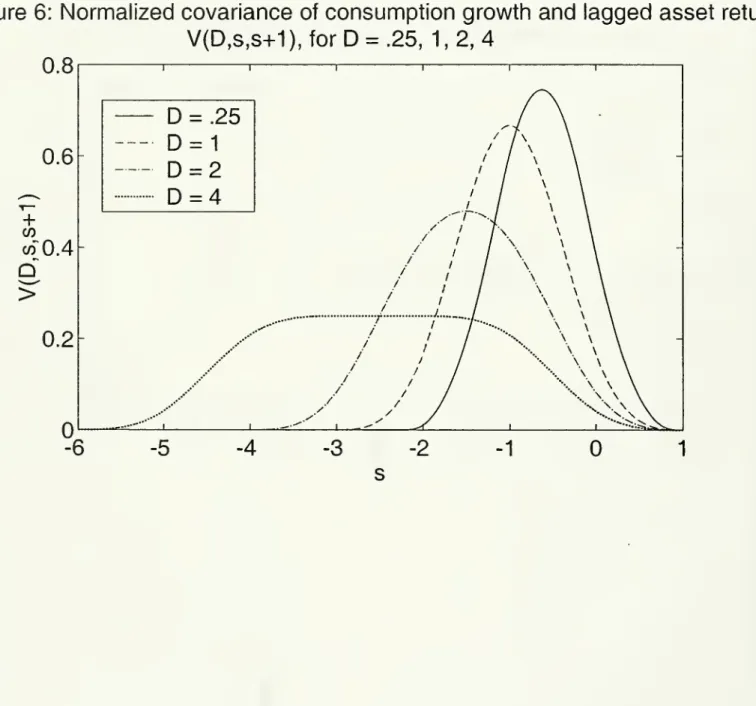
1.

Figure 6 plots the normalized covariances ofconsumption growth

and

lagged asset returns for

different values of D. Specifically,

we

plot

V{D,s,

8

+

1) against s for Z?

=

.25, 1,2,4, from right to left.

Insert Figure 6 about here.

Considera regressionof

consumption

growth

on

some

arbitrary (large)

number

oflaggedreturns,

\nCt+i/Ct

=

_{J2^s^^^t+i+s.}

s=s

One

should find,

p^

=

ev{D,s,8

+

\).

Note

that the

sum

ofthe normalized lagged covariances isone,

q^

Y1

ctw(lnqt,t+i]/C|t_i,£],ln/?|(+s,j+s+i])=

_Y^

V{D,s,8

+

l)

=

l.

s=—00 s=—00

This implies that the

sum

ofthe coefficients will equal the portfolio share of the stock market,15

E

^^

=

^- (1"^)

s=-D-l

3.4

Extension

to

multiple

assets

and

heterogeneity

in

D.

We

now

extend the

framework

to the empirically relevant case ofmultiple assets with stochastic

returns.

We

also introduce heterogeneity in D's.

Such

heterogeneity

may

arise becausedifferent D's apply to different asset classes

and

because

D

may

vary across consumers.

Say

that there are different types ofconsumers I

=

1,...,n;

and

different typesof asset accounts

m

=

l...nm-

Consumers

of type / exist in proportion _{pi (X^iP;}

—

1)

^^^

look at account

m

every

Dim

periods.

The

consumer

has wealth

wim

investedin account

m,

and

has an associated marginal

propensity to

consume

[MFC),

aim- In

most

models the

MFC's

will

be

the

same

for all assets,

but for the sake ofbehavioral realism

and

generality

we

consider possibly different

MFC's.

For instance,

income

shocks could have a low

D

=

I, stock

market

shocks a higher

D

=

4,

and

shocks to housing wealth a.

D

=

40.^^ Account

m

has standard deviation

am, and

shocks

dz^. Call

_Pmn

=

cov{dznt,dzmt)/dt the correlation matrix oftheshocks

and

amn

—

Pmn^rn<^n their

covariance matrix.

'^This is truein a world withonly equities andriskless bonds. In general, it's more appropriate to usea model

withseveralassets, includinghumancapital,as in thenext section.

'^This example implies different short-run marginal propensities to consume out ofwealth windfalls in different asset classes. Thaler (1992) describes one behavioral model with similar asset-specific marginal propensities to

consume.

Totalwealth inthe

economy

is

_{^imPi'^im and}

total

_{consumption YLumPi^imWim-}

A

useful

and

natural quantity is

^Ira

=

^F^ (J-OJ

A

shock dzjnt in wealth account

m

will get translated at

mean

interval

^

^i

Pi

Dim

intoa

consump-tionshock

dC/C

=

_Yl,i

^imdz-mt-We

can calculatethe second

moments

ofour economy.

Theorem

8 In the

economy

described above,

we

have,

ccw{\nCt/Ct-i,lnR^t^^^t^^^^)

=

Yl^imOmnV{Dim,si,S2)

+

o{e^f^^

(19)

and

cav{lnCt+h/Ct+h-iMCt/Ct-i)

=

^

e/m^Pm'^mm'riAm,

Dum',h)

+

O

(e^/^) (20)

1,1',m,m'

with

T{D,

D',h)

=

-^

[d{D

+

h)

+

d(Z?'

-

h)

-

d(D'

-

D

-

h)

-

d{h)\ (21)

and

V

defined in (14), d defined in (11).

The

function T{D,t), defined earher in (10), relates to

T{D,D',t)

by

T{D,D,t)

=

r{D,t).

Recall that

V{D,0,

1)

=

l/h{D). So a conclusion from (19) is that,

when

there are several t3rpes

of people

and

assets, the bias that the econometrician

would

find is the

harmonic

mean

of the

individual biases b{Dim), the weights beinggiven

by

the "shares of variance."

As

an application, consider the case with identical agents (n;

=

1, / is suppressed for this example)

and

different assets with the

same

MPC, Om

=

a. Recall that

V{D,0,

1)

=

l/b{D). So,

the bias

_7/7

will be:

Hence, with several assets, the aggregate bias is theweight

mean

ofthebiases, the

mean

beingthe

harmonic mean, and

the weight of asset

m

being the share ofthe total variance that

comes from

this asset. This allows us, in

Appendix

B, to discuss a modification of the

model

with differential

attention to big shocks (jumps).

These

relationships are derived exactly along the lines ofthe single asset, single type

econ-omy

ofthe previous sections. Expression (19) is the covariance

between

returns, Ini?^,^ ^ ,

—

(T„Z|J_|_^

j^-s 1

+

O

(e),

and

the representation formulafor aggregate consumption.

InCt/Ct-i

=

Y,^mcrm

_[

a(i)z[r_i+,_p„,,_i+,jciz

+

0{e^^^), (23)

where

a{i)

=

(1

—

\i\) . Equation (23) can also be used to calculate the autocovariance (20) of

consumption, ifone defines:

r{D,D',h)=

/ a{i)a{j)cov _{{z[t_i+i_j^^t_-^+,^,zn_-i_^j+h-D',t-i+j+h])}

Ti—j-

(24)

Ji,je[-i,i]

^

J^

(26) 3.5

Sketch

of

the

proof

Proofsofthe propositions appearintheappendix. In thissubsection

we

provideintuition forthose

arguments.

We

start with the following representation formulafor

consumption

growth.

Proposition

9

We

have,

/I

1

InCt+i/Ct

^9a

a{^)z^t+,^D,t+^]^di

+

0{e). (25)

Note

that the order of

magnitude

of9a_{f_^}a{i)zu_^.i_p_t+i]^ is theorder of

magnitude

ofcr, i.e.

O(v^).

Assets returns can

be

represented as _{In i?|(+sj f+g^]}

=

<Jz^^_^.g^^^s^^

+

0(e). So

we

get

cot;(ln^,ln/?[3+3,,3+^2])

/I

(^j

a{i)cov(2|t_!+,_£,,£_i+j],2[s+3j,s+s2]) -^

+

0(e^^^)

/I

di

a{i)X{[t

-1+i-

D,t-l +

i]n[s

+

si,s

+

S2])

—

₍₂₇₎

-1

^

'

+0(e3/2).

Here

A(7)isthe length (the

Lebesgue

measure)ofinterval I. Likewiseonegetscot'(lnCh+t/C/i+(_i,lnCt/Ct_i)

=

9^a^

f

I

a{i)a{j)\{[h

+

t-\

+

i-D,h+t-\+i]f^[t-l+j-D,t-l+j])^-^+o(e^l'^y

The

bulkofthe proofisdevotedto theexplicit calculation ofthis last equation

and

equation (27).

4

Endogenizing

D

Until now,

we

have

assumed

that

D

is fixed exogenously. In this section

we

discuss

how

D

is

chosen,

and

provide a

framework

for calibrating

D.

Becauseofdelayed adjustment, the actual

consumption

path will deviate

from

the "first-best"

instantaneously-adjusted

consumption

path. In steady-state, the welfare loss associated with this

deviationis equivalent, using

a

money

metric, to a proportional wealth loss of

Ac

where'^

Ac

=

^E'

[

—

;-I

+

higher order terms. (28)

Here

AC

is the difference

between

actual

consumption

and

first-best instantaneously adjusted

consumption. Ifthe asset is observed every

D

periods,

we

have

Ac

=

\-i9^o''~D

+

O

(e^) . (29)

Thisisa second-orderapproximation. SeeCochrane (1989) fora similar derivation.

Equations (28)

and

(29) are derived in the appendix.

We

assume^^ that each

consumption

ad-justment _{costs q} proportion of wealth, w.

A

sensiblecalibration ofq

would be

qw

=

(l%)(annual consumption)

=

(.01)(.04)ti;

=

(4 •_10""*)it;.

The

NPV

of costs as a fraction of current wealth is

_q'^n>o^~'^^^

implying a total cognitive

cost of

A

=

^-The

optimal

D

minimizes

both consumption

variability costs

and

cognitive costs, i.e.

D*

=

argminAc

+

Ag.

D*

=

arg

min

--iO^a^D

+

^

—

^r

D

4 1

-

e-P^

so

-70

G

=

qp -pD QP (1

-

e-pDy

Qp (ePO/2

_

e-P^/2)'

4sinh2^

and

we

find for the optimal

D

D*

-

arg sinh

P

A

_f±

6a

y

7p

QP 2^2

^0^a

(30)

when

/9 Z? -C 1.

We

make

the following calibrationchoices: _g

=

4•10"'*, ct^

=

(0.16)^,

7

=

3,

p

=

0.01, tt

=

0.06,

and

9

—

n/{-ya'^)

=

0.78. Substitutinginto our equation for

D,

we

find Z)

~

2 years.

This calibration implies that

D

values of at least 1 year (or 4 quarters) are quiteeasy to defend.

Moreover, our formula for

D*

ishighlysensitivetothevalue of6. Ifaliquidityconstrained

consumer

has only a small fraction ofher wealth inequities

—

because

most

ofher wealth is in other forms

like

human

capital or

home

equity

—

then the value of

D

will be quite large. If

=

.05 because of liquidity constraints, then

D*

~

30 years.

Note

that formula (30)

would

work

for other types ofshocks than stock market shocks.

With

several accounts indexed

by

m,

people

would pay

attention to account

m

at intervals of length

Dr, ^

U QrnP

(31)

''This wouldcomefrom autilityfunction

U =

E

I-9E'

1— »

r

„l-7

1-7

-ds

ifthe adjustment to consumption are madeat dates (Ti)^^^.

A

session of consumption planning at time t lowers

with

qmWm

representing the cost of evaluating asset tti,

and

Om

generahzed as in equation (18).

Equation (31)

impHes

sensible comparative statics

on

the frequency ofreappraisal.

Thus

we

get a

mini-theory ofthe allocation ofattention across accounts.'^

5

Consequences

for

macroeconomics

and

finance

5.1

Simple

calibrated

macro model

To

draw

together the

most

important implications ofthis paper,

we

describe asimple

model

ofthe

US

economy.

We

use our

model

to predict the variability of

consumption

growth, the

autocorre-lation of

consumption

growth,

and

the covariance ofconsumption growth with equity returns.

Assume

the

economy

iscomprisedof

two

classes ofconsumers:stockholders

and

non-stockholders.

The

consumers that

we

model

in section 2 are stockholders. Non-stockholders

do

not have any

equity holdings,

and

instead

consume

earnings from

human

capital. Stockholders have aggregate

wealth St

and

non-stockholders have aggregate wealth Nt- Total

consumption

is given by the

weighted

sum

Ct^a{St

+

Nt).

Recall that

a

is the marginal propensity to consume.

So,

consumption

growth can be

decomposed

into

dC/C

=

sdS/S

+

ndN/N.

Heresrepresentsthewealthofshareholdersdividedby thetotalwealthofthe

economy

and

n

=

1

—

s

represents the wealth of non-shareholders divided

by

the total wealth of the economy.

So

s

and

n

are wealth shares for shareholders

and

non-shareholders respectively.

We

make

the simplifying

approximation that s

and n

are constant in the empirically relevant

medium-run.

Using a first-order approximation,

\n{Ct/Ct-i)

=

sln{St/St-i)

+

nln{Nt/Nt-i).

Ifstockholdershaveloadinginstocks 9, theratioof stock wealthto totalwealthinthe

economy

is.

=

s9. (32)

To

calibrate the

economy

we

begin with the observation that

human

capital claims about 2/3 of

GDP,

Y. In this model,

human

capital is the discoimted net present value of labor

income

accruing to the current cohort of non-stockholders.

We

assume

that the expected duration of

the remaining working lifeof a typical worker is 30 years, implying that the himian capital of the

current work-force is equal to

/30

2 2fl

-

e-^°'')

H

=. _/

_e-^'-y

dt

=

-^^—^

'-Y

~

17F,

7o 3 3r

' _{SeeGabaix andLaibson (2000a,}

b) for abroadertheoretical and empirical analysis of attentionallocation.

" Thisisata givenpointintime.

A

majorreasonfornon-participationisthatrelativelyyoungagentshavemostof

theirwealthinhumancapital,againstwhich they cannot borrowtoinvest inequities(seeConstantinides,Donaldson and Mehra 2000).

where

Y

isaggregateincome. Capital

income

claims 1/3of

GDP.

Assuming

that it has theriskiness (and thereturns) of the stock market, the

amount

ofcapital is

K

=

—^

—

tF

~5y

3(r

+

7r)

so that the equity share oftotalwealth is

By

assuming that all capital is identical to stock

market

capital,

we

implicitly increase the

pre-dicted covariance

between

stock returns

and consumption

growth.

A

more

realistic

model would

assume

a

more

heterogeneous capital stock,

and

hence a lower covariance

between

stock returns

and consumption

growth.

In this

model

economy,

we

work

with data atthe quarterly frequency.

We

assume a

=

.16/\/4,

IT

—

.06/4, r

=

.01/4,

and 7

=

3, so the equity share (equation (1) above) is 6*

=

-k/{"fu'^)

=

.78.

Then

equation (32) implies s

=

.28. In other words,

28%

of the wealth in this

economy

is

owned

by

shareholders. All of stockholders' claims are in either stock or risk-free bonds.

To

keepthings

simple,

we

counterfactually

assume

that A'^

and

S

are uncorrelated.

We

have to take a stand

on

the distribution of

D'

s inthe economy.

We

assume

that

D

values

are uniformly distributed

from

to

D

=

120 quarters (i.e., 30 years).

We

adopt this distribution to capture awide range ofinvestment styles.

Extremely

active investors will have a

D

value close

to 0, while passive savers

may

put their retirement wealth in aspecial mental account, effectively

ignoring theaccumulating wealth until after age 65 (Thaler 1992).

We

are agnosticaboutthe true

distribution of

D

types,

and

we

present this

example

for illustrative purposes.

Any

wide

range of

D

values

would

serve to

make

our key points.

To

keep the focus

on

stockholders,

we

assume

that non-stockholders adjust their

consumption

instantaneously in response to innovations in labor

income

—

i.e., at intervals of length 0.

Theorem

3 implies that thequarterly volatility of aggregate

consumption growth

is.

al

=

n2r(0,

0)a%

+

O'a^

_[

_f

_{_}

T{D, D'

,

0)^

J JD,D'e\0,D]

D

We

assume

that the quarterly standard deviation of

growth

in

human

capital is ai\/

=

.01.^^

Our

assumptions jointly imply that

ac

=

.0063.^^

_Most

of this volatility

comes from

variation in the

consumption

of non-stockholders. Stockholders generate relatively httle

consumption

volatility because they represent a relativelysmall share oftotal

consumption

and

because they only adjust

consumption

every

D

periods. This adjustment rule

smooths

out the response to wealth

innova-tions, since only fraction -^ ofstockholders adjust their

consumption

during

any

singleperiod

and

the average adjustment is of

magnitude

VD.

Our

model's implied quarterly

consumption

volatility

—

_ac

=

0.0063

—

lies below its

empiri-cal counterpart.

We

calculate the empirical

ac

using the cross-country panel dataset created

by

"'Wecalibrate

a^

frompost-

War

U.S.dataon wagegrowth. From1959-2000thestandarddeviationofper-capita

real wage growth at the quarterly frequency has been .0097 (NationalIncome and Product Accounts, Commerce

Department, BureauofEconomicAnalysis). Ifwages follow arandom walk, then thestandard deviationofgrowth

inhuman capital,aif , willequal thestandard deviationin wagegrowth.

--Figure 3 plots the function r(D,0). Note that r(0,0)

=

2/3 and that r(r»,0)

~

l/r>.for large D. In the

Campbell

(1999).^'^

We

estimate

_uc

—

0.0106by averaging acrossallofthe countriesinCampbell's

dataset: Australia,

Canada,

France,

Germany,

Italy, Japan, Netherlands, Spain, Sweden,

Switzer-land, United

Kingdom, and

U.S.^'' Part of the gap

between

our theoretical standard deviation

and

the empirical standard deviation

may

reflect

measurement

error, which should systematically

raise thestandard deviation ofthe empirical data. In addition,

most

ofthe empirical

consumption

series include durables,

which

should raise the variability of

consumption

growth

(Mankiw

1982).

By

contrast, the

US

consumption

data omits durables

and

for the

US

we

calculate

ac

=

0.0054,

closely matching our theoretical value.

Next,

we

turntothefrrst-orderautocorrelationof

consumption

growth, applying again

Theorem

3:

Pc

=

corr(lnCt/Ct-i,lnCt-2/Cf_i)

dDdD'

{oir'

n^ol,V{Q, 1)

+

e^a^

_{f f}

_

Y{D, D'

, 1)-J Jd,D'€[0,D]

d'

Using our calibration choices, our

model

implies

pQ

=

0.34.'^^ This theoretical prediction lies well abovethe empirical estimate of —0.11, found

by

averaging across the country-by-country

autocor-relations inthe

Campbell

dataset.

Here

too, both

measurement

error

and

theinclusion ofdurables are likely to bias the empirical correlations down. Again, the

US

data, which omits durables,

comes

much

closer to

matching

our theoretical prediction. In the

US

data,

_Pq

=

0.22.

We

turn

now

to the covariation

between

aggregate

consumption

growth

and

equity retiu^ns

cov{lnCt/Ct-i,lnRt).

We

find

cov{\nCt/Ct-u\nRt)

=

ea^

_/

_{_}

y(D,0,

1)-=-

=

0.13 10

Jd€\o.d]

D

assuming

that in the short-run the

consumption

growth ofnon-stockholders is uncorrelated with

the

consumption

growth ofstockholders.

The

covariance estimate of 0.13• 10~^ almost

matches

theaveragecovarianceinthe

Campbell

dataset, 0.14-10"''. This time, however,theU.S. data does

not "outperform" the rest ofthe countries in the

Campbell

dataset. For the U.S., the covariance

is 0.60 • 10~^. However, _all of these covariances

come

much

closer to matching our

model

than

to

matching

the

benchmark model

with instantaneous adjustment/measurement.

The

benchmark

model

with

no

delayed adjustment predictsthat the quarterly covariancewill be 60'^

~

₅₀• 10~^.

What

would

an econometrician famihar with the

consumption-CAPM

hterature conclude if

he observed quarterly data from our

QD

economy, but thought he were observing data from the

benchmark economy?

First, he might calculate,

^

=

1000

' _{cov{\iiCt/Ct-i,\nRt)}

~

and

concludethat thecoefficient ofrelative riskaversion is over one-thousand. Ifhe werefamiliar with the

work

of

Mankiw

and

Zeldes (1991), he might restrict his analysis to stockholders

and

calculate,

cm;(ln

St/St-i,m

Rt)

23

We

thank JohnCampbell forsharing thisdatasetwith us.

"We

use quarterly data from the Campbell dataset. Thequarterly databegins in 1947 for theUS, and begins

closeto 1970 formostoftheother countries. Thedataset endsin 1996.

"The

respectiveeffectsaren^(j^r(0,1)

=

.077•IQ-* and

6^(7^

/d.d'61o,dir(^.-D',

1)^^^ =

.048 10^^

Finally, ifheread

Mankiw

and

Zeldescarefully, he

would

realizethathe shouldalso

do

acontinuous time adjustment (ofthe type suggested

by

Grossman

et al 1987), leading to another halving ofhis

estimate. But, after all ofthishard work, he

would

still

end

up

with a biased coefficient of relative

risk aversion: 300/2

=

150. For this economy, the true coefficient ofrelative risk aversion is 3!

These

observations suggest that the literature on the equity

premium

puzzle should

be

reap-praised.

Once

onetakes account ofdelayed adjustment, highestimates of

7 no

longer

seem

anom-alous. Ifworkers in mid-life take decades torespond to innovations in their retirement accounts,

we

should expect naive estimates of

₇

that are far too high.

Defenders oftheEuler equation approach might arguethat economists can go

ahead

estimating

the valueof

_{7 and}

simply correct those estimates forthe biases introduced

by

delayed adjustment.

However,

we

do

not view this as a fruitful approach, since the adjustment delays are difficult to

observe or calibrate.

For an active stock trader,

knowledge

ofpersonal financial wealth

may

be updated

daily,

and

consumption

may

adjust equally quickly.

By

contrast, for the typical employee

who

invests in a 401(k)plan,retirementwealth

may

be

inits

own

mental account,^^

_and

_hence

_may

_not

_be

_integrated

into current

consumption

decisions. This generates lags of decades or

more

between

stock price

changes

and consumption

responses.

Without

precise

knowledge

ofthe distribution of

D

values, econometricians will

be

hardpressed to accurately

measure 7

using the Euler equation approach.

In

summary,

our

model

tells us that high

imputed 7

values are not

anomalous

and

that high frequency properties ofthe aggregate data can

be

explained

by

a

model

with delayed adjustment. Hence, the equity

premium

may

not

be

a puzzle.

Finally,

we

wishto notethat our delayed adjustment

model

is

complementary

tothetheoretical

work

ofother authors

who

have analyzed the equity

premium

puzzle.^^

Our

qualitative approach

has

some

similarity with the habit formation approach (e.g., Constantinides 1990,

Abel

1990,

Campbell

and Cochrane

1999). Habit formation

models

imply that slow adjustment is optimal

because households prefer to

smooth

the

growth

rate (not the level) ofconsumption. In our

%D

model, slow adjustment isonlyoptimal becausedecisioncosts

make

highfrequency adjustment too

expensive.

6

Review

of related

empirical

evidence

In this section,

we

review

two

types of evidence that lend support to our model. In this first

subsection

we

review survey evidence

which

suggests that investors

know

relatively little

about

high frequency variation in their equity wealth. In the second subsection

we

show

that equity

innovations predict future

consumption

growth.

6.1

Knowledge

of equity

prices

Consumers

can't respond to high frequency innovations in equity values if they don't keep close

tabs

on

the values of their equity portfolios. In this subsection,

we

discuss survey evidence that

suggests that

consumers

may

know

relatively little about high frequency variation in the value of

their equity wealth.^*

We

also discuss related evidence that suggests that consumers

may

not

-''SeeThaler (1992).

-^For otherproposedsolutions tothe equitypremiumpuzzleseeKocherlakota(1996), BernartziandThaler(1995),

and Barberisetal (2000).