HAL Id: hal-02778070
https://hal.archives-ouvertes.fr/hal-02778070
Submitted on 12 Nov 2020
HAL is a multi-disciplinary open access
archive for the deposit and dissemination of sci-entific research documents, whether they are pub-lished or not. The documents may come from teaching and research institutions in France or abroad, or from public or private research centers.
L’archive ouverte pluridisciplinaire HAL, est destinée au dépôt et à la diffusion de documents scientifiques de niveau recherche, publiés ou non, émanant des établissements d’enseignement et de recherche français ou étrangers, des laboratoires publics ou privés.
under experimental conditions strengthens bioenergetic
estimate
Marie Vagner, Aurélie Dessier, Christine Dupuy, Paco Bustamante,
Emmanuel Dubillot, Christel Lefrançois, Elodie Réveillac, Pierre Morinière,
Sébastien Lefebvre
To cite this version:
Marie Vagner, Aurélie Dessier, Christine Dupuy, Paco Bustamante, Emmanuel Dubillot, et al.. Maturation of the European sardine Sardina pilchardus under experimental conditions strength-ens bioenergetic estimate. Marine Environmental Research, Elsevier, 2020, 160, pp.104985. �10.1016/j.marenvres.2020.104985�. �hal-02778070�
Maturation of the European sardine Sardina pilchardus under experimental conditions strengthens bioenergetic estimate
Marie Vagnera,1, Aurélie Dessiera, Christine Dupuya, Paco Bustamantea,b, Emmanuel Dubillota, Christel Lefrançoisa, Elodie Reveillacc,2, Pierre Morinièred, Sébastien Lefebvree
aLittoral Environnement et Sociétés (LIENSs), UMR 7266, CNRS-La Rochelle Université, 2
rue Olympe de Gouges, 17042 La Rochelle Cedex 01, France
b Institut Universitaire de France (IUF), 1 rue Descartes 75005 Paris, France
c Agrocampus Ouest, UMR985 ESE Écologie et Santé des Écosystèmes, 65 rue de Saint-
Brieuc, CS 84215, Rennes Cedex 35042, France
d Aquarium La Rochelle, Quai Louis Prunier, 17002 La Rochelle, France
e Université́ Lille, CNRS, Université Littoral Côte d’Opale, UMR 8187, LOG, Laboratoire d’Océanologie et de Géosciences, F-62930 Wimereux, France
*Corresponding author. E-mail address: marie.vagner@univ-brest.fr Tel: +33(0)298 22 43 89
1 Present address : CNRS, Univ Brest, IRD, Ifremer, Laboratoire des sciences de
l’environnement marin (LEMAR), UMR 6539, place Nicolas Copernic, 29 217 Plouzané, France
2 Present address : Littoral Environnement et Sociétés (LIENSs), UMR 7266, CNRS-La
Abstract
This study aims at (1) experimentally estimating first sexual maturation of the European sardine
S. pilchardus, (2) using the results to calibrate existing bioenergetic models. During the 183
days-experiment, fish growth and body condition were assessed by biometry, and gonads were weighed when present. Age, wet weight and total length at first maturity were estimated at 262 days, 10.79 ± 0.75 g, and 11.26 ± 0.21 cm, respectively. Including these traits in biphasic Von Bertalanffy models did not significantly improve simulations for either length or weight data, meaning that energy allocation was not impacted by these traits. The implementation of the results in the Dynamic Energy Budget (DEB) calibration procedure strengthened the parameter set of the existing model, but resulted in significant changes in the energy allocation. Our results are a first step that will allow the design of new experiments to further quantify maturation and reproduction rates in diverse environmental conditions, consolidating DEB model calibration.
Keywords: Bioenergetic modeling, otoliths, first sexual maturity, length-weight relationship, small pelagic fish
1. Introduction
Small pelagic fishes such as the European sardine Sardina pilchardus have a strong worldwide economic and ecological importance, as (i) they represent about 20% of global landings of capture fisheries (Ganias, 2014), and (ii) they play a key role in maintaining ecological processes in marine systems, occupying an essential intermediate trophic level in pelagic ecosystems (Bakun, 2006). The populations of sardines display typically strong fluctuations in abundance within their distribution area (Lluch-Belda et al., 1989; Schwartzlose et al., 1999). This can lead to considerable changes in the functioning of the ecosystems, as well as in fisheries (Food and agriculture organization of the United Nations, 2014). These fluctuating abundances, linked to fluctuating stock structure, actually rely on survival and growth rates of the different life-stages, as well as on the reproductive potential of adults, as a function of food resources and abiotic conditions such as temperature (Alheit and Hagen, 1997; Checkley et al., 2009; van der Lingen et al., 2006). The reproductive potential of adults is directly influenced by their first sexual maturity (or puberty), which is the transition from juvenile to adult stage. In particular, the age and length at first sexual maturity partly determine the duration of the reproductive cycle, the duration of the spawning period, and the quantity of spawning stock in the first year of reproduction (Amenzoui et al., 2006; Sinovčić et al., 2008). For example, it has been shown that smaller individuals reached puberty later, displayed a shorter spawning season, and a lower fecundity than larger individuals at the year scale (Amenzoui et al., 2006; Sinovčić et al., 2008). Also, in different populations, length at first sexual maturity has also been related to the maximal length (Lmax) the fish would reach if they would continue to grow indefinitely
(Beverton, 1992; Froese and Binohlan, 2000; Stamps et al., 1998).
The age and length of sardines at first maturity have been previously estimated from specimens taken from the natural environment (Mustać and Sinovčić, 2010; Saraux et al., 2019; Silva et
al., 2006; Sinovčić et al., 2008, 2003). The first maturity has been shown to generally occur during the end of the first year of life or within the second year (ICES, 2008; Roos, 2009; Sinovčić et al., 2003), but the length at this age varied strongly. Mean length at first sexual maturity (L50, when half of the individuals are mature) was estimated between 10.9 cm and 16.8
cm in the Atlanto-Iberian waters, which extend from the Gulf of Cadiz to the northern French waters (i.e. Northern Bay of Biscay; Silva et al., 2006). Later, Alheit and Petitgas (2010) reported a mean L50 of 14 cm for the same area. More in the south, Amenzoui et al. (2006)
reported a L50 of 15.8 cm in the Atlantic Moroccan coast, while 7.9 cm was the L50 reported for
the Adriatic sea (Sinovčić et al., 2008). This high area-dependent variability of length at first maturity is classically attributed to the influence of environmental conditions, such as food availability and temperature (Amenzoui et al., 2006; Silva et al., 2006; Sinovčić et al., 2008). If these environmental conditions govern the life history trade-off between maintenance, growth and reproduction, they also partly influence the reallocation of energy from the organs used as storage sites (muscle, liver, and/or viscera) towards gonad development and other reproductive costs (Morgan, 2004). In consequence, the first sexual maturity would lead to a decrease of the body condition just before and/or during the maturation process (Amenzoui et al., 2006; Morgan, 2004; Sinovčić et al., 2008; Sinovčić and Zorica, 2006).
First sexual maturity is thus of primary interest to understand the variability in stock structure. In particular, the relationships between growth, age, and bioenergetics at first sexual maturity are critical parameters to consider in bioenergetic models used in fish stocks assessment models (e.g. Jennings et al., 1999). In simple models such as the Von Bertalanffy one (von Bertalanffy, 1957), somatic growth is determined by the balance between energy assimilation and its utilization for body maintenance, asymptotic size being reached when both are equal. After first sexual maturity, reproduction costs are either a subset of the somatic body maintenance or additional costs. In the latter case, a breakpoint is observed in growth trajectories than can be
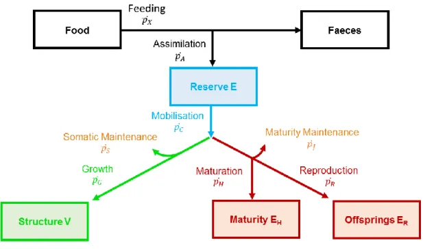
modeled by a biphasic extension of simple models (before and after first maturity) (Brunel et al., 2013; Wilson et al., 2018). In a more mechanistic and complex way, the DEB theory ambitions to capture the quantitative aspects of the metabolism of any animal species from a set of three ordinary differential equations which depend on food resources and processes controlled by temperature (Sousa et al., 2010). Assimilated energy is first stored in a reserve compartment, which is then mobilized to fuel two fluxes with a fixed allocation rule along life span: i) somatic growth and its maintenance on one side and ii) maturity maintenance and maturation (in embryos and juveniles), or reproduction (in adults) on the other side. DEB theory includes classical Von Bertalanffy models as special cases at constant food conditions (Kooijman et al., 2008). Biphasic growth models and dynamic energy budget (DEB) theory display a high sensitivity to the partition of energy to growth, maintenance and reproduction parameters in terms of age and length or weight at maturity but for different reasons. In biphasic growth models, age at first maturity initiates costs of reproduction at the expense of somatic growth, while in DEB models, it stops the increase in maturity level (transition from juvenile to adult stage) and initiates the investment in reproduction without impacting growth. These bioenergetic models are usually calibrated using field data. Some classical Von Bertalanffy (e.g. Silva et al., 2008) and DEB models (Gatti et al., 2017; Nunes et al., 2017) were already parameterized for S. pilchardus following this strategy. However, these model calibrations can also be challenged or even improved using experiments under controlled conditions as this allows a detailed quantification of some processes, such as the size at puberty (De Cubber et al., 2019).
To date, several experimental studies were successful to maintain adult sardines in captivity during several months (Bandarra et al., 2018; Caldeira et al., 2014; Garrido et al., 2007; Goetz et al., 2015; Iglesias and Fuentes, 2014; Marçalo et al., 2013, 2008; Olmedo et al., 1990; Queiros et al., 2019). In particular, some studies experimentally described their survival rate, growth
rate, body condition, lipid reserves (Queiros et al., 2019), ingestion capacity (Caldeira et al., 2014; Garrido et al., 2007; Silva et al., 2014), and stress behavior (Goetz et al., 2015; Marçalo et al., 2013). Reproductive function has also been explored experimentally: gonad maturation of adults and unaided spawning have been observed in captivity (e.g. Bandarra et al., 2018; Marçalo et al., 2008; Queiros et al., 2019), and the post-ovulatory follicle formation, as well as egg and larvae development have been described (Iglesias and Fuentes, 2014; Miranda et al., 1990; Perez et al., 1992). But to our knowledge, none of them have quantified the transition from juvenile to adult stage of S. pilchardus in captivity.
In this context, the objective of the present study was to use an experimental approach to gain quantitative information on the transition from juvenile to adult phase of the European sardine
S. pilchardus from the Bay of Biscay. More specifically, we experimentally studied the
weight-length growth and its relationships with age during a 6-months period, including the first sexual maturity. Then, these new data were used to challenge and/or to strengthen parameter estimations of two categories of bioenergetic models: classic and biphasic Von Bertalanffy models, and DEB models. New DEB model estimates were confronted to existing ones (Nunes et al., 2017; Gatti et al., 2017). This study will provide better knowledge for management actions of the sardine stock in the very large Bay of Biscay located in the North-East Atlantic Ocean, which supports a rich biodiversity and abundance of marine species, and in which S.
pilchardus represents one of the most important fisheries
2.Material and methods
2.1. Ethics statement
All fish manipulations were performed according to the Animal Care Committee of France (ACCF) and performed at the Aquarium of La Rochelle facilities. Permissions were required from departmental service of fisheries to collect sardines in their natural environment (authorization n°99–1216). The protocol was approved by the ACCF. All fish manipulations were performed under anaesthesia, and all efforts were made to minimize suffering during manipulation.
2.2. Fish harvest and experimental rearing conditions
2.2.1. Fish harvest
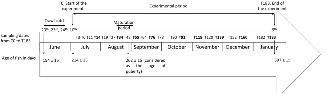
The chronology of experimental design is presented in Fig. 1. A total of 250 fish was sampled in natural environment, during three days of sampling. S. pilchardus were trawled by a commercial purse-seiner operating from the port of La Rochelle in the Pertuis d’Antioche (France) on June 20th, 23rd 24th2014 and transferred at the Aquarium of La Rochelle facilities. Among the 250 fish collected, some individuals were randomly collected in the catches to be weighed and measured at each sampling period (n = 27 fish the 20th June; n = 29 fish the 23 and n= 29 fish the 24th June). On the fishing vessel, all fish were placed into aerated 50 L tanks
(~100 individuals per tank) and anesthetized (2-Phenoxyethanol, 99%, Fisher Scientific, Illkirch France) to reduce stress during transportation to Aquarium of La Rochelle premises.
2.2.2. Experimental rearing conditions
Once arrived at the Aquarium of La Rochelle, the 250 fish were transferred into one large rearing tank (8700 L) for the experimentation. During the acclimation period which lasted between 17 and 20 days (from fish arrival to the Aquarium, i.e. from 20th 23rd or 24th of June, until the beginning of the experiment, i.e. the 10th of July), fish were daily fed ad libitum with both alive Artemia sp. nauplii and frozen cyclops (600 g day-1 for the entire rearing tank, Cyclops, Ocean Nutrition, Essen, Belgium).
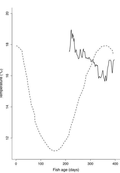
After the acclimation period, the experimentation extended from the 10th July 2014 (T0) until the 9th January 2015 (183 days, i.e. T183). Fish were maintained in a semi-open recirculating system allowing a daily water renewal rate of 1% and submitted to a single sanitary treatment using Hydrogent® (0.056 mL L-1, GERFO, France) and Tenotryl® (0.02 mL L-1, Virbac France, France). Water tank temperature was monitored continuously during the experiment (HOBO Pro v2, Onset, Massachusetts, USA), and was 17.1 ± 0.8°C (Fig. 2), corresponding to the temperature observed in June in Pertuis d’Antioche and staying within the temperature range of the Bay of Biscay presented in Gatti et al. (2017, Fig. 2). Fish were exposed to a 12L:12D photoperiod cycle. Water salinity (Practical Salinity Unit) was weekly measured (30.6 ± 1.6 p.s.u.; ODEON salinometer, PONSEL Mesure, France). Fish were daily fed ad libitum with 100 g day -1(for the entire tank, i.e. varying between 7.6% of biomass at the beginning of the experiment to 2% of biomass at the end of the experiment, which was considered ad libitum) of commercial pellets (Aquafirst 15, TYCA, France) of 0.5 mm diameter (for details on its composition, see Table S1). Feeding was executed by an automatic dispenser placed above the tank. The mortality rate at the end of the experiment was 2% (i.e. n = 5 fish found dead in total).
2.3. Age estimation
During the fish sampling in the trawled site, a total of 18 individuals of S. pilchardus was collected on the 20th, 23rd, 24thJune 2014 (n = 6 individuals per sampling date) for further age
estimation (in days, Fig. 1). Fish were first anesthetized (2-Phenoxyethanol, 99%, Fisher Scientific, Illkirch France), and then sacrificed on board by an overdose of the anesthetic. Left sagittal otoliths were extracted and preserved dry in vials pending analysis, which were further performed at the fisheries ecology laboratory of the UMR ESE in Agrocampus Ouest (France). Otoliths were then embedded individually on microscope slides in thermoplastic epoxy resin (Crystal Bond©509). To expose inner growth increments, otoliths were polished with a 3 m
lapping film (ESCIL© MOA3). They were then photographed at X400 magnification with a camera- equipped microscope (Zeiss©Primo Star coupled to AxioCam ERc 5s). Image analyses
(ImageJ©) allowed at counting growth increments along the post-rostrum axis. Age interpretation was made using the group band reading (GBR) method as recommended by the Working Group on micro-increment daily growth in European Anchovy and Sardine (ICES, 2013).
2.4. Fish sampling during the experiment
2.4.1. Total length and wet weight on alive individuals
In order to follow individual fish growth along the experimental period, 24h-unfed fish were randomly caught into the rearing tank at n = 9 sampling times: T14, T34, T55, T76, T97, T118, T139, T160 and T183 days (Fig. 1); 22 to 32 individuals were sampled at each time using a landing net. These fish were placed in a well-aerated maintenance tank of 50 L containing experimental tank water and Stress Coat solution 0.2 mL L-1 (Poisson d’Or, Belgium) used to
protect fish skin and prevent the loss of scales. Fish were then individually anesthetized using tricaine metanesulphonate MS-222 (0.3 g L-1; Sigma-Aldrich, Saint Quentin-Fallavier, France)
under oxygenation before being weighed (W in g) and measured (total length, i.e. L, in cm). They were then transferred into a recovery tank filled with water from the experimental tank, under constant oxygenation and containing Hydrogent® solution (0.056 mL L-1, GERFO,
France) to avoid any bacterial contaminations due to manipulation. Once the recovery was completed, fish were transferred back to their experimental tank.
2.4.2. Fish hematocrit and gonad weight on sacrificed individuals
Following a logarithmic scale (at T0, T3, T6, T11, T19, T27, T48, T64, T78, T90, T120, T152, T182 days of the experimental period, Fig. 1), five 24h-unfed fish were randomly sampled in the rearing tank using a landing net (i.e. 13 samplings were done over the six months of the experimental period). This number of five was selected as a compromise in order to have a representative number of individuals, while limiting the change in the group organization (initially n = 250 fish, and n = 185 fish at the end of the experiment). Indeed, changes in schooling structure (fish density, shape …) may have physiological consequences for the individuals of this gregarious species, such as variations in swimming activity and associated energy costs. The five fish were anesthetized with tricaine metanesulphonate MS-222 (0.3 g L
-1; Sigma-Aldrich, Saint Quentin-Fallavier, France) to be weighted and measured, as described
above. Then, blood was rapidly sampled by caudal puncture using chilled heparinized syringes (heparin concentration: 35-40 mg mL-1, Sigma-Aldrich, Saint Quentin-Fallavier, France). Hematocrit (percentage of red blood cells in the centrifuged blood volume) was determined in duplicate in capillary tubes centrifuged for 3 min at 3000 g at 4°C. Fish were sacrificed by prolonged anesthesia.
Fish were dissected and when present, gonads were removed and weighed. The gonadosomatic index (GSI, % of fresh fish weight) using the following relationship (1):
𝐺𝑆𝐼 = 100 (𝑊𝑔𝑜𝑛𝑎𝑑
where 𝑊𝑔𝑜𝑛𝑎𝑑 is the weight of gonad and W, the wet weight of the 24h-unfed individuals. Fish with developing gonads were considered to be mature (Silva et al., 2006). The age at first maturity was considered as the age at which at least 50% of the population was mature.
2.5. Fish condition over the experiment
2.5.1. Body condition index and statistics
Biometrics provided by 2.4.1 and 2.4.2 (n = 327 individuals) during the experiment (≥ T0),
added to those obtained from fish sampled on the 20th, 23 and 24th June (n = 87 individuals)
before the experiment started, formed the total length and wet weight database used in calculations below (i.e. n = 414 in total).
The relationship between the total length (L, in cm) and wet weight (W, in g) was determined for each fish, according to the equation (2; Ricker, 1973):
W = aLb (2)
where, a is a constant, the shape, and b is an allometric coefficient.
For each fish, the relative condition index of Le Cren (Kn, Le Cren, 1951, equation 3) was used as a proxy of individual condition. It was chosen because it prevents from the assumption of isometric growth and avoid a potential length effect:
Kn = Wstandard W (3)
where W is the mass of an individual and Wstandard is the theoretical mass of an individual of a given total length (L) predicted by the length-weight relationship described in equation (2). The higher the Kn index value, the better the condition of the fish.
The effect of experimental conditions on Length-Weight relationships and Le Cren index (comparing the data before and after T0) were performed with ANCOVA on Log W and Log
Normality and homoscedasticity were tested on residuals using Shapiro-Wilk and Bartlett test, respectively.
2.5.2. Bioenergetic modeling
2.5.2.1. Von Bertalanffy modeling (biphasic and classic)
The fish growth was modeled using a biphasic model depending on time described by a set of two equations for juveniles and adults, respectively. The switch depends on time at maturity (tmat) such as in Brunel et al. (2013) but follows Von Bertalanffy laws (von Bertalanffy, 1957),
giving for W:
𝑊𝐽(𝑡) =(a/b-(a/b- 𝑊(0) 1
3
⁄ ) e ^ (-b/3 t))^3 for t ≤ t
mat i.e. juvenile stage (4)
𝑊𝐴(𝑡) = ( 𝑎 𝑏+𝑐− ( 𝑎 𝑏+𝑐− 𝑊(𝑚𝑎𝑡) 1 3 ⁄ ) 𝑒−𝑏+𝑐 3 (𝑡−𝑡𝑚𝑎𝑡)) 3
for t > tmat i.e. adult stage (5)
where:
- Tmat was set at when 50% of fish were mature,
- WJ(t) and WA(t) are W, as a function of time (t) for juvenile and adult, respectively,
- W(0) and W(mat) are W at time 0 and at tmat, respectively,
- a, b, c are the size-specific rates of energy acquisition and energy use for body maintenance and reproduction, respectively, a and b being common for juvenile and adult stages.
The typical Von Bertalanffy parameters, asymptotic weight Wmax and growth rate KVB can be
retrieved as follow for juvenile and adult respectively: 𝑊𝑚𝑎𝑥𝐽 = (𝑎 𝑏) 3 𝑎𝑛𝑑 𝑊𝑚𝑎𝑥𝐴 = ( 𝑎 𝑏+𝑐) 3 (6) and 𝐾𝑉𝐵𝐽 = 𝑏 𝑎𝑛𝑑 𝐾𝑉𝐵𝐴 = 𝑏 + 𝑐 (7)
For length data, equations are written as follow: 𝐿𝐽(𝑡) =𝑎 𝑏− ( 𝑎 𝑏− 𝐿(0)) 𝑒 −𝑏 𝑡 for t ≤ t
mat i.e. juvenile stage (8)
𝐿𝐴(𝑡) = 𝑎 𝑏+𝑐− ( 𝑎 𝑏+𝑐− 𝐿(𝑚𝑎𝑡)) 𝑒 −(𝑏+𝑐)(𝑡−𝑡𝑚𝑎𝑡) for t > t
mat i.e. adult stage (9)
where:
- LJ(t) and LA(t) are L as a function of time (t) for juvenile and adult, respectively,
- L(0) and L(mat) are L at time 0 and at tmat, respectively,
- a, b, c are the size-specific rates of energy acquisition and energy use for body maintenance and reproduction, respectively, a and b being common for juvenile and adult stages, with: 𝐿𝑚𝑎𝑥𝐽= 𝑎 𝑏 𝑎𝑛𝑑 𝐿𝑚𝑎𝑥𝐴 = 𝑎 𝑏+𝑐 (10)
A temperature effect was introduced in the equations as proposed by Fontoura and Agostinho (1996) but following the correction of the DEB theory. All rates (a, b, c) were temperature corrected using the Equation (11), where TA is the Arrhenius temperature (K), 𝑘̇1 the rate of
interest at the reference temperature Tref (293.15 °K), and 𝑘̇ the rate of interest at temperature T
(in °K). TA was fixed at 9800 °K as in the DEB calibration procedure.
𝑘̇(𝑇) = 𝑘̇1exp ( 𝑇𝐴
𝑇𝑟𝑒𝑓−
𝑇𝐴
𝑇) (11)
L0(t) and W0(t) were settled using the mean of the observed values at t0. The 𝑡𝑚𝑎𝑡 was settled
thanks to the experiment. Fitted parameters are then a, b and c. If the effect of tmat is not
significant, the equation for juvenile applies for adults too and parameters are re-calibrated on the full dataset following then a classical Von Bertalanffy model (i.e. c=0).
All the growth curve fitting processes and associated statistics were coded in R v.3.5.3 (2019). As temperature varied every day at different rates (Fig. 2), first-order ordinary differential equations (ODE) of Equations (1) and (2) were preferred to simple iteration procedures.
Equations were resolved using the package deSolve (
https://CRAN.R-project.org/package=deSolve). Parameter estimations was then performed using an optim()
function that minimizes a symmetric bounded loss function (Marques et al., 2018). Standard errors of parameters were evaluated using a bootstrap method with 100 random sampling with replacement of the original data sets. Results are presented using mean with standard error (mean ± SE). All fittings were tested by analysis of variance (significant from α < 0.001), and parameter significance by t-test.
2.5.2.2. DEB modeling
A general presentation of the theory and its mathematical formulation is presented in supplementary material (Text S1). Two DEB models were already parameterized for Sardina
pilchardus. First an abj-DEB model was parameterized using the co-variation method (Lika et
al., 2011) and code is freely available
(https://www.bio.vu.nl/thb/deb/deblab/add_my_pet/entries_web/Sardina_pilchardus/Sardina_
pilchardus_res.html; Nunes et al., 2017). Compared to the standard version (std), the abj model
considers a metabolic acceleration between birth and metamorphosis (see S1). Available parameters for this first model are summarized in Table 1A and it will be named AMP_old hereafter. Parametrization was initially done on life history traits, such as age, length, weight at some life stages (called zero-variate data in DEB terminology, see Table 1B), and univariate data such as length over time or age and length-weight relationships (Table 1C). These data originated from studies on S. pilchardus done in the Atlanto-Iberian waters (eg. Silva et al., 2006, 2008; Nunes et al., 2011) and were selected at the appreciation of the authors. Except for some L-W measurements, it is worth noticed that all zero and univariate data were provided from in situ estimations. Second, a std model was developed on this species by Gatti et al. (2017) using only in situ data and following a different calibration procedure that further
benefits from parameters of another species (the European anchovy, Engraulis encrasicolus; Gatti et al., 2017). A metabolic acceleration was considered on assimilation flux (𝑝̇𝐴) only (and
not concomitantly on the energy conductance) by multiplying 𝑝̇𝐴 with a correcting factor (corL):
corL = min (1, max (L-Lb + (Lj-L facc), facc)) (12)
with the acceleration factor (facc = 0.1), the structural length (L) at birth (Lb = 0.028 cm) and at
juvenile stage (Lj = 0.84 cm). Gatti et al. (2017) calibrated eight parameter sets to their
observations. The closest to the observations of the present experiment (see result section for details) is also available in Table 1A.
Simulations using the parameters of these two studies and a new parameter set were confronted to the experimental data of the present study. Hence, one new parameterization procedure following the covariation method (Lika et al., 2011) was performed by integrating results from the present study, i.e. age, length and weight at first sexual maturity (Zero variate data, Table 1B), as well as total length and wet weight versus age (Univariate data, Table 1C) to the data present in the original code of Nunes et al. (2017) (AMP_Old) which were kept identical. However, the original age, weight and length at first sexual maturity were weighed by a zero factor and the new data from the present study were weighed by a ten factor.
The new estimation of parameters (hereafter named AMP_New) was completed using the package DEBtool (as described in Marques et al., 2018) on the software Matlab R2010b. The parameter estimation procedures were evaluated by computing the Mean Relative Errors (MRE), varying from 0, when predictions match data exactly, to infinity when they do not, and the Symmetric Mean Square Errors (SMSE), varying from 0, when predictions match data exactly, to 1 when they do not (Marques et al., 2018). As maturity level (EH) cannot be estimated
(i.e. total length, and wet weight versus age) started with initial values at birth (L=Lb, E=Eb, H=
𝐸𝐻𝑏, R=0 and ab= 6 days) with the respective values of the three parameters sets. From age 6 to
age 194 (i.e. before the harvest), temperature followed the one predicted by Gatti et al. (2017, Fig. 2). From age 194 to age 214 days (i.e. the start of the experiment), temperature was assumed to be 17°C, and from age 214 days onwards temperature was monitored daily (Fig. 2). For simplicity, the scaled functional response (f) of AMP_New which was calibrated during the estimation procedure, was also used for AMP_Old to produce the simulations on the univariate data of the present experiment. However, the scaled functional responses for Gatti et al. (2017) parameter sets were adjusted to fit the observations.
Calculations of physical length, wet or dry weight, or gonad wet weight from state variables of the DEB theory are provided in supplementary material. For Gatti et al. (2017), wet weight was estimated as the sum of dry weight, water mass (Wm) and ash mass (Wa), the two latter varying
with physical length (Lw, cm) and total energy content (Etot, kJ), following their own
methodology:
Wm=exp (-0.84 + 0.2*Lw + 0.28*ln(Etot) - 0.008*Lw*ln(Etot)) (13)
Wa=exp (-2.93 + 0.91*ln(Wm))
In all cases, energy in reproduction (ER) was not considered into the calculation of wet or dry
weights. As spawning was not modeled in our model, this could potentially lead to an overestimation of the contribution of reproduction to weight.
3. Results
3.1. Age estimation of fish
At sampling at sea, the age of the 18 juveniles averaged 187.0 ± 11.6 days, 199.7 ± 16.1 days and 203.2 ± 17.7 on June 20th, 23rdand 24th2014, respectively. These estimates correspond to
a common birth date in December 2013, arguing that all the individuals belong to the same cohort. Thus, the mean age of all the individuals collected was estimated at 194.3 ± 15.4 days on the 20th of June. Their mean age was estimated to be 214.3 ± 15.4 days at the start of the
experiment (T0, i.e. the 10th of July, Fig. 1), and 397.3 ± 15.4 days at the end of the experiment (T183).
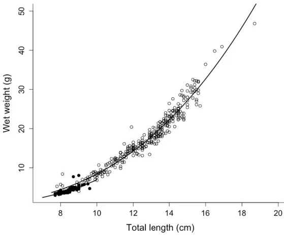
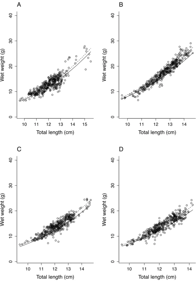
3.2. Length-weight relationships
The TL-W relationship was described (Fig. 3) as W = 0.0111 x TL2.96 (R2 = 0.63, n = 86, P<0.001) before the experiment (i.e. before T0, Fig. 1) and W = 0.0076 x TL2.88 (R2 = 0.96, n =
326, P<0.001) during the experiment. Shape coefficients were significantly different (aov, P<0.001) but not the allometric coefficients (P = 0.745). There was, in average, a 5-fold increase in W and 1.7-fold increase in L from T20 to T183 (Fig. 3).
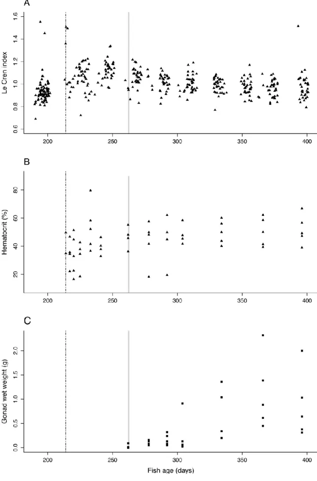
3.3. Fish condition and maturation process
Values for Le Cren relative condition index Kn, hematocrit and gonad weight of S. pilchardus
over the experiment period are summarized in Fig. 4.
Kn was significantly higher during the experimental period (from T0) than before (aov: Le Cren:
F1, 412 = 47.08, p-value = 2.5 x10E-11; Fig. 4A). It was 0.93 ± 0.11 mg mm-3(min-max:
0.69-1.55) before the experiment, and 1.03 ± 0.12 mg mm-3 (min-max: 0.721 – 2.12) during the experiment. All along the experiment, Le Cren index remained stable (lm: time-effect: F1, 325 =
0.12, p-value = 0.7; Fig. 4A). This observation was associated with a mean percentage of hematocrit of 44.30 ± 1.69 %, which slightly increased during the experimental period (lm: F1, 54 = 8.80, p-value = 4.0 x 10E-3; Fig. 4B).
The gonad weight showed that the fish became mature between T34 (last sampling before T48) and T48 (at which 80% of fish were mature, Fig. 4C). At T48, the first gonads were developed
on four out of the five dissected fish. Thus, T48 (262.2 days of age; fish W = 10.79 ± 0.75 g, fish L = 11.26 ± 0.21 cm) was considered as age of first maturity. Between T48and T183, i.e. during the adult period of the experiment, the GSI averaged 2.83 ± 2.18 % (min-max: 0.11-7.95, not presented here). The maximum value of GSI observed over the experiment was 7.95% and was recorded at T152 (366.2 days of age).
3.3.1. Bioenergetic: Von bertalanffy models
As the Kn fish body condition index significantly differed between before and during the
experiment, only observations from T0 onwards were used for parameterization of the Von
Bertalanffy biphasic models. Tmat was set at 48 days, when 4 out of 5 of sampled fish were
mature). The average estimation of weight and length at T0 for the experimental population
were W0 = 5.22 ± 0.38 g, and L0 = 8.30 ± 0.47 cm, respectively.
Von Bertalanffy biphasic models were significant for both wet weight (W) and total length (L) measurements (Table 2). However, the two “c” parameters (rates for reproduction) were negative for wet weight and total length, respectively, indicating that the model is inconsistent and over-parameterized. Consequently, a classic Von Bertalanffy model was applied (equations (4) and (6) for juveniles) and similarly performed (Table 2 and Fig. 5A and B). Then, it is concluded that maturity did not provoke a change in the allocation energy strategy under these experimental conditions. Estimated Wmax and Lmax were 29.05 ± 3.10 g and 15.25 ± 0.81 cm,
respectively, and the Von bertalanffy growth rates (KVB = b) at 20°C equal 0.054 ± 0.004 d-1,
0.0178 ± 0.000 d-1 for wet weight and total length, respectively. Note that estimated shape from VB parameters (Wmax = 0.0082 Lmax3) is very close to the one estimated directly from
3.3.2. Bioenergetic: DEB Modeling
Life history traits at puberty used for the initial parameterization (AMP_Old) originated from estimations from in situ data. They were somewhat different than the ones measured in the present experimental study, while temperatures were roughly the same (Table zero variate, Table 1B). In the present study (AMP_New), length at puberty was slightly shorter (Lp2 = 11
cm < Lp = 13 cm) and weight at puberty was half lower than for AMP_Old (Wp2 = 9.8 g <<
Wp.= 20 g). Note that zero variate data are selected on the basis of no food limitation in the
DEB calibration procedure (i.e. scaled functional response, f = 1). This is why the lowest values of L and W of the five individuals sampled at T48 (age at first maturity = 262 d) were selected (Table 1B), i.e. the individual that reached maturity the sooner. Another important change was age at puberty (i.e. first maturity) which was set at 262 days (at 14.4°C) in AMP_New from the present experiment, instead of 365 days (at 15°C) initially used in AMP_Old (note that this value was estimated from in situ data).
After re-parameterization of the AMP data set, fits were excellent for the vast majority of zero-variate (Table 1B) and unizero-variate data (Table 1C and Figs. S2 and S3), both AMP_Old and AMP_New parameter sets (Relative errors are low; Table 1B and 1C), with the exception of the maximum reproduction rate which was underestimated by the new parameterization (RE is 0.59). Drastic changes in parameters occurred for allocation to growth () from 0.33 to 0.89 and maturity level (E_Hp) from 74890 to 3065 J. It is worth to mention that the maximum
assimilation rate (Pam) decreased by half while somatic maintenance rate (Pm) increased by
66%. The acceleration rate (sM) increased by 65% too. Finally, all scaled functional responses
(f) for in situ data are now comparable (f ca. 0.8-0.9) with the AMP_New, and below 1, which is now coherent. Note that the f value for uni-variate data is typically around 0.8 as these data are estimated from populations and that all individuals cannot feed ad libitum. As for quality of predictions, the mean relative errors have approximately doubled (from 0.08 to 0.194
between AMP_Old and AMP_New mostly due to the RE of the maximum reproduction rate) and the symmetric mean square errors have tripled (from 0.086 to 0.224). However, these values are still good keeping in mind that new datasets (three zero-variate and two uni-variate data) were implemented in the parameterization code.
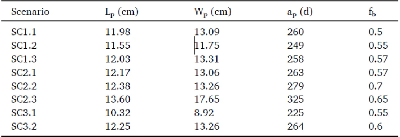
In their study, Gatti et al. (2017) calibrated eight different parameter sets for which simulations were performed in the conditions of our experiment. The parameter sets performed roughly the same for length or weight simulations (see Fig. S4), but differed a lot in the predictions of age, length and weight at puberty (Table 3). Range of values were 225–325 days, 10.3–13.6 cm, and 8.9–17.7 g for age, length and wet weight at puberty. The scenario SC1.2 was the closest to the observations of the present experiment (zero-variate data Table 1B and uni-variate data Fig. 4A and B) and was selected for further comparisons with AMP_Old and AMP_New. In particular, simulations of total length and wet weight of the present experiment with the three parameter sets (AMP_Old, AMP_New, and Gatti et al., 2017; SC1.2) were comparable with close values of scaled functional response (f from 0.7 to 0.86; Fig. 5A and B).
The SC1.2 parameter set differs mostly from AMP_Old and New in six main aspects of bioenergetics. κ was between the two other parametrizations (0.65); the volume specific costs of structure and the specific maintenance rate were lower than AMP_new by 28% and 70% respectively; the maturity maintenance rate, the energy conductance and the maturation threshold for puberty were one order of magnitude higher than AMP_New parameter set.
4. Discussion
The present work shows that S. pilchardus was successfully reared in experimental conditions during six months, and were under favorable growth conditions enabling the cohort to perform its first sexual maturation transitioning from juvenile to adult stages. This original experiment
enabled to strengthen the existing bioenergetic models, by tuning the estimation of DEB parameters of a small pelagic fish of high ecological and economic interests.
4.1. Ageing
The birth date determined in December 2013 in the present study is consistent with observations for S. pilchardus in the wild. Our estimates of age-length relationship based on this birth date determination are in the range of the age-length relationship previously proposed by Silva et al. (2015) for the same species.
4.2. Fish growth during the experiment
The mean linear growth rate determined for juveniles in the present work (0.06 cm day-1 from T0 to T48 of the experiment) was about 30% higher than the growth rate previously estimated for S. pilchardus juveniles obtained from the wild (Alemany et al., 2006: 0.04 cm day-1 in the Alboran sea; Silva et al., 2015: 0.041 cm day-1 in the Western coast of Portugal). This difference would be mainly explained by the ad libitum feeding of fish during our experimental period. Also, the lower energetic constraints (such as foraging activity, routine swimming speed or escape from predators) encountered by fish in experimental conditions than in the wild at both juvenile and adult stages, could explain this difference. We cannot indeed rule out that metabolic process and trade off in energy allocation may probably differ between individuals held in experimental conditions and those growing in completely wild conditions. In that respect, it is worth noticing that the growth dynamics observed in our experiment was similar to that obtained in captivity by Iglesias and Fuentes (2014), and the size (14.5 cm) at 397 days of age similar to that presented in their study.
4.3. Fish body condition during the experiment
Fish appeared healthy all over the experimental period, as shown by the condition factors measured (Le Cren relative index and hematocrit). The values of hematocrit are in the same range as those already found in healthy sardines (Marçalo et al., 2006) and rainbow trouts (Trenzado et al., 2009). The slight increase of the hematocrit values measured all along the experiment suggest the absence of stress and the good health status of fish. Stressed fish usually display high hematocrit variability. In addition, an acute stress usually leads to a reduction in hematocrit values in sardine, probably as a result of hemodilution (Marçalo et al., 2008, 2006). This hemodilution is likely due to enhanced gill permeability to seawater in response to stress, leading to the potential for seawater to shift between tissues and blood (Marçalo et al., 2008, 2006). The good health status of the fish during the present experiment is in accordance with the Kn index values, which increased from the capture to the experimental period. The Kn values
obtained were in the same range as those reported (ranging from 0.73 to 1.43) for the same species by Brosset et al. (2015).
Our results show that the Kn index seems to slightly decrease during the maturation period,
before stabilizing until the end of the experimental period. Such a decrease during the maturation period has already been reported for this species (Brosset et al. 2015), and would be interpreted as the reallocation of fat content towards gonad maturation.
During our experiment, adipose tissue was observed until the apparition of gonads but seemed to decrease in mass after gonadic maturation process (visual observations). As gonad development of sardines is known to be dependent on past resources (Ganias, 2014, 2009), this fat deposits have certainly been accumulated both during life period spent in natural environment and during the first weeks of experiments, before being reallocated towards gonad maturation. This result also testifies the good natural initial health status of fish, enabled by the good experimental conditions (no predator, no competition, and no food limitation). In our
study, the fish weight and the GSI index have been measured in not-gutted individuals, including reserves of organs used as storage sites (muscle, liver, and/or viscera). The part of fish reserves that have gone specifically from the muscles to the gonads is therefore unknown. The steady Kn observed until the end of our experiment may reflect a steady fish weight but not
necessarily a steady fish condition as a large part of fish reserves may have moved from muscles to gonads during this whole period, and this reallocation may have differed according to maturity stages and sexes.
4.4. Sexual maturation
In the present study, we considered that fish first maturation occurred at 262 days-old, i.e. within the first year of life, which is in accordance with what is usually described in the Bay of Biscay and Adriatic sea (Alheit and Petitgas, 2010; Roos, 2009; Sinovčić et al., 2003). However, it is slightly overestimated as in the experiment, 80% of individuals matured between age of 238 days old (T34 of the experiment) and 262 days old (T48). The development of gonads from mid-August in our experimental conditions corresponds to the natural seasonal pattern of GSI for sardines in Adriatic sea and Aegean sea (Mustać and Sinovčić 2009; Nunes et al., 2011b). It is also in accordance with what is usually found in the Bay of Biscay, where mature sardines are found year round (Alheit and Petitgas, 2010). Gonad wet weights (from 0.1 in July to 1.2 in December) and GSI (from 0.5 in July to 4.5% of the body weight in December) measured in our study were in the same range as those previously reported by Mustać and Sinovčić (2010) for S. pilchardus in the Adriatic Sea. However, as we calculated GSI using not-gutted fish, it may have been under-estimated in our study.
In the present study, first maturity was reached at a slightly lower length (T48, 11.26 ± 0.21 cm) than usually observed in the Bay of Biscay (around 14 cm, Alheit and Petitgas, 2010; Silva
et al., 2006). It has been reported to be about 12 cm in the Mediterranean Sea (Roos, 2009; Saraux et al., 2019) until 2009, but about 9.6 cm after 2009 (Saraux et al., 2019), 9.92 cm in the Aegean Sea (Nikolioudakis et al., 2014), and around 8 cm in Adriatic sea (Sinovčić et al., 2008, 2003). Silva et al. (2008) pointed out that sardine populations are genetically homogeneous in the Atlanto-Iberian waters, although some degree of spatial population structuring may be due to local environmental conditions. As maturation period and length at maturity are controlled by many other factors, among which biotic (quality and quantity of food …) and abiotic factors such as temperature during the juvenile phase (Taranger et al., 2010; van der Lingen et al., 2006), this result clearly supports that an adequate supply and quality of food (higher than in natural environment) associated to the good quality of abiotic environment (i.e., temperature) provided in the present experiment allowed the sardine to mature at a smaller size than usually reported in the Bay of Biscay.
4.5. Bioenergetics
Including age at first maturity determined in the present study in biphasic Von Bertalanffy models did not show any effects on energy allocation towards growth. This is in line with DEB theory in which the allocation to growth and its maintenance is a fixed proportion of mobilized reserves whatever the life stages (see Text S1). Then, the maximum length of ca 15.3 cm estimated using a classical Von Bertalanffy model is in the common size range usually reported in the Bay of Biscay (between 15 and 25 cm; maximum: 28 cm; Coiffec, 2006; Silva, 2003). It was, however, well under what was previously estimated using Von Bertalanffy growth model in the Alboran sea (Alemany et al., 2006) and in the Gulf of Lions (Van Beveren et al., 2014), with 24 cm and from 18.38 cm to 33.57 cm, respectively. Using a Gompertz growth model, Silva et al. (2015) estimated an even lower theoretical maximum length (14.3 cm) than us for
sardines from the northwest coast of Portugal. The narrow range of observations in total length or weight in the present study certainly prevented from getting realistic estimates of the asymptotic weight and total length although the temperature forcing was included in the model. However, AMP_New for Sardina pilchardus predicts an ultimate length of 26.3 cm in satiety conditions (f = 1) and of 22.6 cm in our experimental conditions (at f = 0.86). All these results suggest that the theoretical maximum length of S. pilchardus could differ according to the growth model used, but could also strongly depend on the home living physico-chemical environment of the sardines, genetic pool (or ecotype). The temperature used in our study (17.1 ± 0.8 °C) was lower than the temperature measured in the Gulf of Lions (Van Beveren et al., 2014) and the Alboran sea (Alemany et al., 2006), but certainly higher than that measured in the northwest coast of Portugal where a cold upwelling occurs (Silva et al., 2006).
The implementation of the results of the present study within the AMP calibration procedure has changed drastically the estimation of DEB parameters in two main directions. First, age, length and weight at puberty were much lower than in the initial dataset, giving a far lower value of the maturity level threshold (25-fold lower). Silva et al. (2008) indicated that Sardine populations are genetically homogeneous in Atlanto-Iberian waters (see above). This potentially means that traits at maturity may have been overestimated in AMP_Old, due to an inaccurate estimation of environmental parameters, and food availability in particular. As a consequence, investment in reproduction is now considered occurring sooner than before. Second, in our study, the maximum assimilation rate decreased by 2, while the mobilization of reserves and somatic maintenance increased in the same proportion, increasing the allocation fraction to soma by 3 times favoring allocation to growth. The consequence is a lower investment in reproduction. The bioenergetics of the species as described by DEB is now rather different and fits better with several other fish species (Kooijman and Lika, 2014). AMP_New also restores coherence in the scaled functional responses of the univariate data that all approach
(f = 0.8–0.9). The only noticeable deviance concerns the maximum reproduction rate. However, this value is extremely difficult to estimate accurately for multiple spawners such as Sardina
pilchardus. In particular, the duration of the spawning season and the frequency of spawning is
still difficult to estimate (Gatti et al., 2017) and then the real reproduction rate is uncertain. So, a significant deviance could be considered as acceptable.
Actually, the uncertainty in reproduction rate leads Gatti et al. (2017) to propose eight different parameter sets based on different scenarios of spawning. All these parameter sets performed approximately the same for length and weight data, but simulated a large range in the values of traits at maturity. Our observations allow to select one parameter set (SC1.2) that was close to our observations but still, the bioenergetics are somewhat different. Although maximum assimilation rates are comparable between SC1.2 and AMP_New, the mobilized reserve is allocated differently. Allocation to growth, specific somatic maintenance and volume specific cost of structure are lower in SC1.2 compare to AMP_New. On the contrary, allocation to maturity/reproduction, energy conductance, maturity maintenance rate and maturation threshold for puberty are much higher. Another difference relies in the structure of the Gatti et al. (2017)’s model which is neither a true standard nor a true abj DEB model: acceleration between birth and juvenile was undertaken differently and only partially than an abj model (cf M&M section). Putting aside this structural difference, the different balances in the allocation of energy are most probably linked to the method of estimation of allocation fraction to soma (κ), the maturity maintenance rate (kJ) and the maturation threshold for puberty (𝐸𝐻𝑝). The calibration procedure of Gatti et al. (2017)’s considered a high value of kJ equal to kM (the
somatic maintenance rate coefficient i.e. the ratio between pM and EG), which implies that
maturity occurs at a fixed length without effect of food availability (Kooijman et al., 2008). On the contrary, in the AMP procedure, it is advised to keep value of kJ low and fixed (Lika et al., 2014). Actually, the only way to better estimate these values whatever the calibration procedure
is to get estimates of reproduction rates and/or length at puberty at different known food rations (Kooijman et al., 2008). Experiments in controlled conditions including different food ration, and during which investment in reproduction and spawning will be measured, would be probably the best way to provide the necessary values to refine bioenergetics in DEB theory and other models in general.
Our study showed that quantifying maturation of S. pilchardus in experimental conditions is possible and further experiments are necessary to estimate accurately reproduction rate. This was a significant first step to refine the parameter sets of the DEB theory that could lead a better management of this species evaluation of stocks and exploitation sustainability.
Acknowledgements
We are especially very grateful to the Aquarium of La Rochelle and its team (special thanks to Jean-François, Romain, Olivier and Vincent) for their advice on animal collecting, maintenance techniques, interest and availability all along the experiment. We thank M. Durollet, J. Lucas, T. Lacoue-Labarthe and I. Percelay for their help in the fish dissections at the laboratory. This study was supported through a PhD grant for A. Dessier from the Conseil Régional de Poitou-Charentes (now Nouvelle Aquitaine) and by the European project REPRODUCE (Era Net-Marifish, FP7). The Institut Universitaire de France (IUF) is acknowledged for its support to PB as a Senior Member.
Fundings
This research was supported by a PhD grant for A. Dessier from the Conseil Régional de Poitou-Charentes (now Nouvelle Aquitaine) and by the European project REPRODUCE (Era Net-Marifish, FP7).
References
Alemany, F., Álvarez, I., García, A., Cortés, D., Ramírez, T., Quintanilla, J., Álvarez, F., Rodríguez, J.M., 2006. Postflexion larvae and juvenile daily growth patterns of the Alboran Sea sardine (Sardina pilchardus Walb.): influence of wind. Sci. Mar. 70, 93–104.
Alheit, J., Hagen, E., 1997. Long-term climate forcing of European herring and sardine populations. Fish. Oceanogr 6, 130–139.
Alheit, J., Petitgas, P. (Eds.), 2010. Life-cycle spatial patterns of small pelagic fish in the Northeast Atlantic, ICES cooperative research report. Internat. Council for the Exploration of the Sea, Copenhagen.
Amenzoui, K., Ferhan-Tachinante, F., Yahyaoui, A., Kifani, S., Mesfioui, A.H., 2006. Analysis of the cycle of reproduction of Sardina pilchardus (Walbaum, 1792) off the Moroccan Atlantic coast. C.R. Biol. 329, 892–901.
Bakun, A., 2006. Wasp-waist populations and marine ecosystem dynamics: Navigating the “predator pit” topographies. Progr. Oceanogr. 68, 271–288.
Bandarra, N.M., Marçalo, A., Cordeiro, A.R., Pousão-Ferreira, P., 2018. Sardine (Sardina
pilchardus) lipid composition: Does it change after one year in captivity? Food Chem. 244,
408–413.
Beverton, R.J.H., 1992. Patterns of reproductive strategy parameters in some marine teleost fishes. J. Fish Biol. 41, 137–160.
Brosset, P., Fromentin, J.-M., Ménard, F., Pernet, F., Bourdeix, J.-H., Bigot, J.-L., Van Beveren, E., Pérez Roda, M.A., Choy, S., Saraux, C., 2015. Measurement and analysis of small pelagic fish condition: A suitable method for rapid evaluation in the field. J. Exp. Mar. Biol. Ecol. 462, 90–97.
Brunel, T., Ernande, B., Mollet, F.M., Rijnsdorp, A.D., 2013. Estimating age at maturation and energy-based life-history traits from individual growth trajectories with nonlinear mixed-effects models. Oecologia 172, 631–643.
Caldeira, C., Santos, A., Ré, P., Peck, M., Saiz, E., Garrido, S., 2014. Effects of prey concentration on ingestion rates of European sardine Sardina pilchardus larvae in the laboratory. Mar. Ecol. Progr. Ser. 517, 217–228.
Checkley, D., Alheit, J., Oozeki, Y., Roy, C. (Eds.), 2009. Climate change and small pelagic fish. Cambridge University Press, Cambridge.
Coiffec, G., 2006. Analyse de la pêcherie des petits pélagiques, sardine et anchois dans le golfe de Gascogne (Rapport de 2ème année). Ifremer.
De Cubber, L., Lefebvre, S., Lancelot, T., Denis, L., Gaudron, S.M., 2019. Annelid polychaetes experience metabolic acceleration as other Lophotrochozoans: Inferences on the life cycle of Arenicola marina with a Dynamic Energy Budget model. Ecol. Model. 411, 108773. Fontoura, N.F., Agostinho, A.A., 1996. Growth with seasonally varying temperatures: an
expansion of the von Bertalanffy growth model. J. Fish. Biol. 48, 569–584.
Food and agriculture organization of the United States., 2014. State of the world fisheries and aquaculture 2014. Food & Agriculture Org.
Froese, R., Binohlan, C., 2000. Empirical relationships to estimate asymptotic length, length at first maturity and length at maximum yield per recruit in fishes, with a simple method to evaluate length frequency data. J. Fish Biol. 56, 758–773.
Ganias, K. (Ed.), 2014. Biology and ecology of sardines and anchovies. CRC Press.
Ganias, K., 2009. Linking sardine spawning dynamics to environmental variability. Est. Coast. Shelf Sci. 84, 402–408.
Garrido, S., Marçalo, A., Zwolinski, J., van der Lingen, C., 2007. Laboratory investigations on the effect of prey size and concentration on the feeding behaviour of Sardina pilchardus. Mar. Ecol. Progr. Ser. 330, 189–199.
Gatti, P., Petitgas, P., Huret, M., 2017. Comparing biological traits of anchovy and sardine in the Bay of Biscay: A modelling approach with the Dynamic Energy Budget. Ecol. Model. 348, 93–109.
Goetz, S., Santos, M.B., Vingada, J., Costas, D.C., Villanueva, A.G., Pierce, G.J., 2015. Do pingers cause stress in fish? An experimental tank study with European sardine, Sardina
pilchardus (Walbaum, 1792) (Actinopterygii, Clupeidae), exposed to a 70 kHz dolphin
pinger. Hydrobiologia 749, 83–96.
ICES, 2016. Report of the Working Group on Southern Horse Mackerel, Anchovy and Sardine (WGHANSA) (No. ICES CM 2016/ACOM:17.). Lorient, France.
ICES, 2013. Workshop on micro increment daily growth in European Anchovy and Sardine (WKMIAS). Sicily, Italy.
ICES, 2008. Report of the Workshop on Small Pelagics (Sardina pilchardus, Engraulis
encrasicolus) maturity stages (WKSPMAT). Mazara del Vallo, Italy.
Iglesias, J., Fuentes, L., 2014. Culture viability of Sardina pilchardus (Fish, Teleost): Preliminary results of growth in captivity up to 18 months. Sci. Mar. 78, 371–375.
Jennings, S., Greenstreet, Simon.P.R., Reynolds, John.D., 1999. Structural change in an exploited fish community: a consequence of differential fishing effects on species with contrasting life histories. J. Anim. Ecol. 68, 617–627.
Kooijman, S.A.L.M., Lika, K., 2014. Resource allocation to reproduction in animals: Resource allocation to reproduction in animals. Biol. Rev. 89, 849–859.
Kooijman, S.A.L.M., 2015. Measurement and analysis of small pelagic fish condition: A suitable method for rapid evaluation in the field., 462 UK: Cambridge University Press, pp. 90–97.
Kooijman, S.A.L.M., Sousa, T., Pecquerie, L., Van Der Meer, J., Jager, T., 2008. From food-dependent statistics to metabolic parameters, a practical guide to the use of dynamic energy budget theory. Biol. Rev. 83, 533–552.
Le Cren, E.D., 1951. The length-weight relationship and seasonal cycle in gonad weight and condition in the perch (Perca fluviatilis). J. Anim. Ecol. 20, 201.
Lika, K., Augustine, S., Pecquerie, L., Kooijman, S.A.L.M., 2014. The bijection from data to parameter space with the standard DEB model quantifies the supply–demand spectrum. J. Theor. Biol. 354, 35–47.
Lika, K., Kearney, M.R., Freitas, V., van der Veer, H.W., van der Meer, J., Wijsman, J.W.M., Pecquerie, L., Kooijman, S.A.L.M., 2011. The “covariation method” for estimating the parameters of the standard Dynamic Energy Budget model I: Philosophy and approach. J. Sea Res. 66, 270–277.
Lluch-Belda, D., Crawford, R.J.M., Kawasaki, T., MacCall, A.D., Parrish, R.H., Schwartzlose, R.A., Smith, P.E., 1989. World-wide fluctuations of sardine and anchovy stocks: the regime problem. S. Afr. J. Mar. Sci. 8, 195–205.
Marçalo, A., Araújo, J., Pousão-Ferreira, P., Pierce, G.J., Stratoudakis, Y., Erzini, K., 2013. Behavioural responses of sardines Sardina pilchardus to simulated purse-seine capture and slipping: Sardina pilchardus responses to capture and slipping. J. Fish Biol. 83, 480–500. Marçalo, A., Mateus, L., Correia, J.H.D., Serra, P., Fryer, R., Stratoudakis, Y., 2006. Sardine
(Sardina pilchardus) stress reactions to purse seine fishing. Mar. Biol. 149, 1509–1518. Marçalo, A., Pousão-Ferreira, P., Mateus, L., Duarte Correia, J.H., Stratoudakis, Y., 2008.
Sardine early survival, physical condition and stress after introduction to captivity. J. Fish Biol. 72, 103–120.
Marques, G.M., Augustine, S., Lika, K., Pecquerie, L., Domingos, T., Kooijman, S.A.L.M., 2018. The AmP project: Comparing species on the basis of dynamic energy budget parameters. PLOS Comput. Biol. 14, e1006100.
Miranda, A., Cal, R.M., Iglesias, J., 1990. Effect of temperature on the development of eggs and larvae of sardine Sardina pilchardus Walbaum in captivity. J. Exp. Mar. Biol. Ecol. 140, 69–77.
Morgan, M.J., 2004. The relationship between fish condition and the probability of being mature in American plaice (Hippoglossoides platessoides). ICES J. Mar. Sci. 61, 64–70. Mustać, B., Sinovčić, G., 2010. Reproduction, length-weight relationship and condition of
sardine, Sardina pilchardus (Walbaum, 1792), in the eastern Middle Adriatic Sea (Croatia). Period. Biol. 112, 133–138.
Mustać, B., Sinovčić, G., 2009. Comparison of mesenteric and tissue fat content in relation to sexual cycle of the sardine, Sardina pilchardus (Walb., 1792), in the eastern Middle Adriatic fishery grounds (Croatia). J. Appl. Ichthyol. 25, 595–599.
Nikolioudakis, N., Isari, S., Somarakis, S., 2014. Trophodynamics of anchovy in a non-upwelling system: direct comparison with sardine. Mar. Ecol. Progr. Ser. 500, 215–229. Nunes, C., Marques, G., Sousa, T., Kooijman, B., Queiros, Q., 2019. AmP Sardina pilchardus. Nunes, C., Silva, A., Soares, E., Ganias, K., 2011. The use of hepatic and somatic indices and histological information to characterize the reproductive dynamics of Atlantic Sardine
Sardina pilchardus from the Portuguese coast. Mar. Coast. Fish. 3, 127–144.
Olmedo, M., Iglesias, J., Peleteiro, J., Forés, R., Miranda, A., 1990. Acclimatization and induced spawning of sardine Sardina pilchardus Walbaum in captivity. J. Exp. Mar. Biol. Ecol. 140, 61–67.
Perez, N., Figueiredo, I., Macewicz, J., 1992. The spawing frequency of sardine, Sardina
pilchardus (Walb.), off the Atlantic Iberian coast. 175–189.
Queiros, Q., Fromentin, J.-M., Gasset, E., Dutto, G., Huiban, C., Metral, L., Leclerc, L., Schull, Q., McKenzie, D.J., Saraux, C., 2019. Food in the Sea: Size Also Matters for Pelagic Fish. Front. Mar. Sci. 6, 385.
Ricker, W.E., 1973. Linear regressions in fishery research. J. Fish. Res. Board Can. 30, 409– 434.
Roos, D., 2009. Les populations ichtyologiques de petits pélagiques / SRM MO.
Saraux, C., Van Beveren, E., Brosset, P., Queiros, Q., Bourdeix, J.-H., Dutto, G., Gasset, E., Jac, C., Bonhommeau, S., Fromentin, J.-M., 2019. Small pelagic fish dynamics: A review of mechanisms in the Gulf of Lions. Deep Sea Res. Part II Top. Stud. Oceanogr.159, 52–61. Schwartzlose, R.A., Alheit, J., Bakun, A., Baumgartner, T.R., Cloete, R., Crawford, R.J.M., Fletcher, W.J., Green-Ruiz, Y., Hagen, E., Kawasaki, T., Lluch-Belda, D., Lluch-Cota, S.E., MacCall, A.D., Matsuura, Y., Nevárez-Martínez, M.O., Parrish, R.H., Roy, C., Serra, R.,
Shust, K.V., Ward, M.N., Zuzunaga, J.Z., 1999. Worldwide large-scale fluctuations of sardine and anchovy populations. S. Afr. J. Mar. Sci.21, 289–347.
Silva, A., 2003. Morphometric variation among sardine (Sardina pilchardus) populations from the northeastern Atlantic and the western Mediterranean. ICES J. Mar. Sci. 60, 1352–1360. Silva, A., Carrera, P., Massé, J., Uriarte, A., Santos, M.B., Oliveira, P.B., Soares, E., Porteiro, C., Stratoudakis, Y., 2008. Geographic variability of sardine growth across the northeastern Atlantic and the Mediterranean Sea. Fish. Res. 90, 56–69.
Silva, A., Santos, M.B., Caneco, B., Pestana, G., Porteiro, C., Carrera, P., Stratoudakis, Y., 2006. Temporal and geographic variability of sardine maturity at length in the northeastern Atlantic and the western Mediterranean. ICES J. Mar. Sci. 63, 663–676.
Silva, A.V., Meneses, I., Silva, A., 2015. Predicting the age of sardine juveniles (Sardina
pilchardus) from otolith and fish morphometric characteristics. Sci. Mar. 79, 35–42.
Silva, L., Faria, A., Teodósio, M., Garrido, S., 2014. Ontogeny of swimming behaviour in sardine Sardina pilchardus larvae and effect of larval nutritional condition on critical speed. Mar. Ecol. Progr. Ser. 504, 287–300.
Sinovčić, G., Keč, V.Č., Zorica, B., 2008. Population structure, size at maturity and condition of sardine, Sardina pilchardus (Walb., 1792), in the nursery ground of the eastern Adriatic Sea (Krka River Estuary, Croatia). Estuar. Coast Shelf Sci.76, 739–744.
Sinovčić, G., Zorica, B., 2006. Reproductive cycle and minimal length at sexual maturity of
Engraulis encrasicolus (L.) in the Zrmanja River estuary (Adriatic Sea, Croatia). Estuar.
Coast Shelf Sci. 69, 439–448.
Sinovčić, G., Zorica, B., Franičević, M., Keč, V.Č., 2003. First sexual maturity of sardine,
Sardina pilchardus (Walb.) in the eastern Adriatic Sea. Period. Biol.105, 401–404.
Sousa, T., Domingos, T., Poggiale, J.-C., Kooijman, S.A.L.M., 2010. Dynamic energy budget theory restores coherence in biology. Phil. Trans. Biol. Sci. 365, 3413–3428.
Stamps, J.A., Mangel, M., Phillips, J.A., 1998. A New Look at Relationships between Size at Maturity and Asymptotic Size. Am. Nat. 152, 470–479.
Taranger, G.L., Carrillo, M., Schulz, R.W., Fontaine, P., Zanuy, S., Felip, A., Weltzien, F.-A., Dufour, S., Karlsen, Ø., Norberg, B., Andersson, E., Hansen, T., 2010. Control of puberty in farmed fish. Gen. Comp. Endocrinol. 165, 483–515.
Trenzado, C.E., Morales, A.E., Palma, J.M., de la Higuera, M., 2009. Blood antioxidant defenses and hematological adjustments in crowded/uncrowded rainbow trout (Oncorhynchus mykiss) fed on diets with different levels of antioxidant vitamins and HUFA. Comp. Biochem. Physiol. C Toxicol. Pharmacol. 149, 440–447.
Van Beveren, E., Bonhommeau, S., Fromentin, J.-M., Bigot, J.-L., Bourdeix, J.-H., Brosset, P., Roos, D., Saraux, C., 2014. Rapid changes in growth, condition, size and age of small pelagic fish in the Mediterranean. Mar. Biol. 161, 1809–1822.
van der Lingen, C., Hutchings, L., Field, J., 2006. Comparative trophodynamics of anchovy
Engraulis encrasicolus and sardine Sardinops sagax in the southern Benguela: are species
alternations between small pelagic fish trophodynamically mediated? Afr. J. Mar. Sci. 28, 465–477.
von Bertalanffy, L., 1957. Quantitative laws in metabolism and growth. Q. Rev. Biol. 32, 217– 231.
Wilson, K.L., Honsey, A.E., Moe, B., Venturelli, P., 2018. Growing the biphasic framework: techniques and recommendations for fitting emerging growth models. Method Ecolo. Evol. 9, 822–833.
Figure 1. Chronology of the experimental design. Bold cases indicate the sampling dates for length and weight measurements during the experimental period (n = 22 to 32 fish per sampling date, fish were not euthanized), while the other sampling dates concern, in addition to length and weight, hematocrit measurement and dissection for gonad weight (n = 5 fish per sampling date fish were euthanized). A total of 87 fish were also measured and weighed during the trawl catch (n = 27 fish on June 20th, n = 30 fish on June 23rd, and n = 30 fish on June 24th). Estimated maturation period (from T34 to T48) is indicated in grey shadow. T48 (i.e. 262 days old) corresponds to the date at which the first gonad development was observed, and T64 (i.e. 278 days old) corresponds to the date at which all specimens observed were mature. The age of fish at T-20, T0 and T183 is indicated as mean days ± SD.
June July August September October November December January
20th, 23rd, 24th Trawl catch 10th T3 T6 T11 T14 T19 T27 T34 T48 T55 T64 T76 T78 T90 T92 T118 T120 T139 T152 T160 T182 T183 9th T0, Start of the experiment T183, End of the experiment Experimental period Maturation period 194 ± 15 397 ± 15 Sampling dates from T0 to T183
Age of fish in days 214 ± 15 262 ± 15 (considered as the age of puberty)
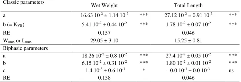
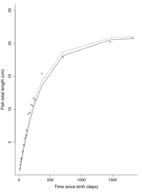
Figure 2. Water temperature. Temperature according to fish age (days) during our experiment (solid line) and during the study of Gatti et al. (2017; dashed line).
Figure 3. The total length (L) – wet weight (W) relationship. Data collected both before (full black circles, n = 87 individuals) and during the experimental period (open black circles; n = 327 individuals) are represented. These relationships are represented by equations W = 0.0111 L2.96 before the experiment, and W = 0.0076 L2.88 during the experiment, and the coefficient
Figure 4. Body condition of Sardinia pilchardus over time. The Le Cren index (A; n = 414), the percentage of hematocrit (B; n = 56), and the gonad weight (C; n = 29 individuals) are represented over the fish age in days. The beginning of the experiment (T0, i.e. 214.3 ± 15.4 days of age) is indicated on the figure by the dotted vertical line. The age of puberty (T48, i.e. 262 days of age) is indicated in light grey vertical line. Concerning the Le Cren index, data from the trawled period were included (before the T0 of the experiment).