Adiabatic Approximation in Explicit
Solvent Models of RedOx Chemistry
The MIT Faculty has made this article openly available. Please share
how this access benefits you. Your story matters.
Citation Vaissier, Valérie and Troy Van Voorhis. “Adiabatic Approximation in Explicit Solvent Models of RedOx Chemistry.” Journal of Chemical Theory and Computation 12, 10 (September 2016): 5111–5116 © 2016 American Chemical Society
As Published https://pubs.acs.org/doi/10.1021/acs.jctc.6b00746
Publisher American Chemical Society (ACS)
Version Author's final manuscript
Citable link http://hdl.handle.net/1721.1/115111
Terms of Use Article is made available in accordance with the publisher's policy and may be subject to US copyright law. Please refer to the publisher's site for terms of use.
The Adiabatic Approximation in Explicit Solvent
Models of RedOx Chemistry
Valérie Vaissier and Troy Van Voorhis
∗Department of Chemistry Massachusetts Institute of Technology
77 Massachusetts Avenue Cambridge, MA 02139
E-mail: [email protected]
Abstract
We propose a calculation scheme that accelerates QM/MM simulations of solvated sys-tems. This new approach is based on the adiabatic approximation whereby the solute degrees of freedom are separated from those of the solvent. More specifically, we assume that the so-lute electron density remains constant with respect to the relaxation of the solvent molecules. This allows us to achieve a dramatic speed up of QM/MM calculations by discarding the slow self-consistent field cycle. We test this method by applying it to the calculation of redox po-tential of aqueous transition metal ions. The root-mean-square deviation (RMSD) between the full solvation and adiabatic approximation is only 0.17 V. We find a RMSD from experimental values of 0.32 V for the adiabatic approximation as compared to 0.31 V for the full solvation model, so that the two methods are of essentially the same accuracy. Meanwhile the adiabatic calculations are up to 10 times faster than the full solvation calculations, meaning the method proposed here reduces the cost of QM/MM calculations while retaining its accuracy.
1
Introduction
Solvent effects influence chemical reactivity by modifying the solute’s fundamental properties such as its charge distribution, stability, solubility and diffusivity. At the molecular level, solute-solvent interactions shape the configuration of the system, which in turns dictates its behavior.1 There-fore, the solvent controls both the thermodynamics and the kinetics of chemical reactions. Protein folding rate for example, core to the enzymatic activity of biological systems, is limited by the dif-fusion of the polypeptide chains in the solvent.2Consequently, adequately capturing the effects of solvation in computational chemistry methods is valuable to many research fields.3–7In particular, electron transfer and reduction-oxydation reactions are processes proven to be extremely solvent sensitive.8–12However, solute and solvent are characterized by more degrees of freedom than can be computed. As a result, models are developed to reduce the number of variables and make the problem tractable while retaining the chemistry of solvation. The solvent degrees of freedom may or may not be included in such formalisms that are then named explicit or implicit solvent models respectively.13,14The latter is largely affordable since, while the solute is treated quantum mechan-ically, only a response to a continuum medium is incorporated to mimic the solute solvent interac-tion.14 The continuum is parametrized to reproduce a macroscopically observed property, namely the dielectric constant as in the polarizable continuum model (PCM) for example.14–17Although very diverse in their implementation, all implicit solvent models rely on an adiabatic approxima-tion in which the solvent instantaneously adjusts to any changes in the charge distribuapproxima-tion of the solute. As a result, the solute degrees of freedom can be separated from the solvent, with the solute experiencing a potential from the average of the solvent configurations. The calculation thus only requires one QM calculation for each solute configuration and disposes with the costly ensemble average over solvent configurations.14 Implicit solvent models are remarkably successful for the calculation of equilibrium energies of solvation but fail to capture the phenomena associated with hydrophobic effects, hydrogen bonds and viscosity.13,18,19In these cases, configurational sampling is crucial and one turns to the more expensive explicit solvent models.13Ideally, one would use an "all Quantum Mechanichal (QM)" approach where both the solute and the solvent are treated at the
quantum mechanical level. Nevertheless, even with progress in linear scaling Density Functional Theory (DFT)20,21the size of the systems with relevance in chemistry and biology quickly prohibit such techniques. Instead one uses quantum mechanical/ molecular mechanical (QM/MM) meth-ods where the solute (and often its first solvation shells) is treated quantum mechanically while the solvent is described classically via a force field that depends only on position and orientation coordinates.6,7,22–26 Nevertheless, QM/MM calculations remain expensive because of the size of the QM region that can still be quite large as well as the non triviality of computing the QM region interaction with the MM region.13,27 Some efforts to reduce the cost of such methods includes decoupling of the QM and MM regions,13,28reducing the effective size of the QM region by freez-ing the shell in contact with the MM region,29–31 perturbation matrix method,32,33 tight binding approaches34,35 as well as the analytical Reference Interaction Site Model (RISM).36
Here, we propose a conceptually simpler QM/MM calculation scheme for redox potential in water, that relies on the same adiabatic approximation as the one used in implicit solvent models. This is achieved by considering the QM electron density fixed while the MM molecules follow regular molecular dynamics steps. We test this adiabatic approximation by calculating the redox potential of transition metal ions in water, a notoriously challenging system that is widely used in catalysis.37,38 People have emphasized that the adiabatic approximation is not valid in general because solute polarization is important for many solvation properties.6,7,39 Here we make the important discovery that, at least for redox potentials of transition metal ions in water, the adia-batic approximation is valid. We report a root-mean-square deviation with conventional QM/MM calculations and experiments of 0.17 V and 0.32 V respectively. We suggest some reasons why this is the case. Furthermore, since this effectively removes the self-consistent field cycle at every QM/MM step, we report a speed up of such calculations by a factor of 10.
2
Computational Methods
2.1
Calculation of redox potential
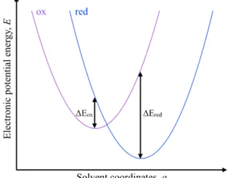
We make use of the linear response approximation19to express the redox potential associated with the reaction ox + e–*)red, Eoxcalc(ox/red), as:
Eoxcalc(ox/red) = 1
2[∆Eox(ox/red) + ∆Ered(ox/red)] , (1)
where ∆Eox and ∆Ered are the absolute energy differences between the oxidized and reduced
species in the oxidized and reduced state respectively (see Figure 1).
Figure 1: Potential energy curves of a redox couple. In the linear approximation, we take the redox potential of the couple as being the average of the absolute energy differences between the oxidized and reduced species in each oxidation state (∆Eox and ∆Ered).
Throughout this paper, we calculate the redox potential of transition metal ions in water asso-ciated with the reaction: [M(H2O)6]3++ e–*)[M(H2O)6]2+where M is one of the following : iron, vanadium, copper, cobalt, manganese, titanium or chromium. We use QM/MM to calculate our energies in which case the energy differences are NVT ensemble averages:
∆Eox(ox/red) = hE(ox) − E(red)iox,NVT (2)
∆Ered(ox/red) = hE(ox) − E(red)ired,NVT (3)
with E(ox) and E(red) are the energies of the oxidized and reduced species respectively. The details of the QM/MM procedure are given below.
2.2
QM/MM calculations
2.2.1 Full solvation
To adequately account for solvation effects, we build a 40 × 40 × 40 Å3water box at the center of which sits the solute. The QM region consists of the metal ion and its first solvation shell: six water molecules arranged in an octahedron. In general (and particularly for copper), the coordination number of the M2+ ions is debated.41 40,42,43We used six QM waters because it is necessary to have the same number of QM atoms for the oxidized and reduced species. Nothing forces the waters to stay coordinated, but we find in practice that they remain hexacoordinate of their own accord. This is not definitive proof that the real system is hexacoordinate but it does say that the theory used here wants them to be hexacoordinate. Therefore, hexaaqua ions are the only internally consistent choice. The structure of this QM subsystem was first optimized with DFT in gas phase (Q-Chem 4.3,44 B3LYP45/lanl2dz46). All QM/MM calculations were performed with the CP2K software package.27 Non polarizable TIP3P force field47 was used for the MM region made of 2141 water molecules. The B3LYP functional in combination with the SZV basis set48 was used for the production of the QM/MM trajectories while DZVP48 was used for QM/MM energy calculations. The combination of B3LYP and a polarized basis set has already been proven accurate for the calculation of redox potential of metal ions.19 For completeness, we show in the Supporting Information that B3LYP predicts a similar energy gap of the hydrated ions than PBE0 (with DZVP). However, PBE/DZVP leads to a systematic underestimation, up to 0.5 eV.
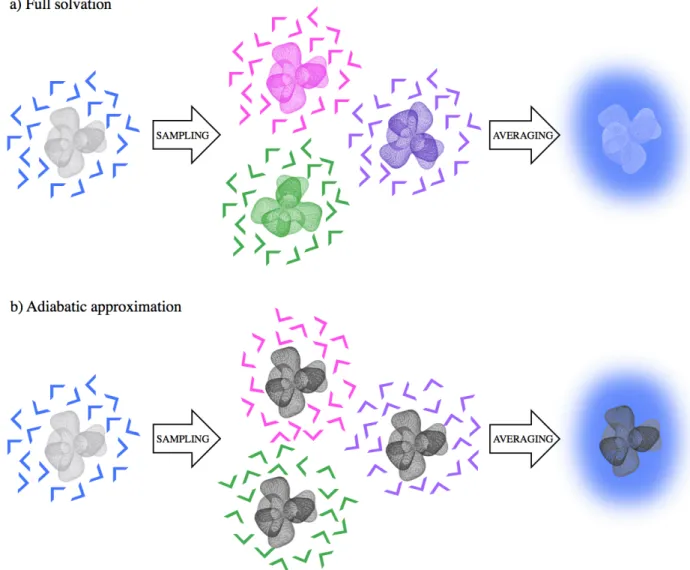
Furthermore, we show that the SZV basis set fails to adequately predict the variations across the series. Periodic boundary conditions were set for the MM waters only, i.e. there were no periodic image of the QM subsystem. In CP2K, the electrostatic QM/MM potential is decomposed in a sum of gaussian functions and a residual term accounting for the long range interactions.39,49,50This is computed with a multrigrid approach as extensively detailed in.49,50In this work, we use four grids with a relative cutoff of 40 Ry. Full details can be found in the input files provided in the Supporting Information. In the regular QM/MM calculation scheme, the electrostatic potential due to the MM waters is included in the Hamiltonian from which the electron density of the solute is computed self consistently at each step (see Figure 2a). The desired observable is eventually calculated by averaging over many configurations of the QM density in equilibrium with the surrounding solvent. From this point on, we will refer to this scheme as the ’full solvation’ scenario. It contrasts with the adiabatic approximation QM/MM calculation scheme described below.
2.2.2 The adiabatic approximation
In this scenario, we use the same set up as for the full solvation but we keep the electron density of the solvent fixed, allowing only for the relaxation of the MM solvent molecules, as illustrated in Figure 2b.
The configuration sampling of the solvent molecules is similar to the full solvation case. Only here the MM water molecules are distributed around the same density step after step. In practice, we ran a very short regular QM/MM trajectory (0.1 picosecond) to get a reasonable solute electron density. An example input file for this case is also provided in the Supporting Information. Ad-ditionally, we present in the Supporting Information the energy gap variations of one of the ions (vanadium) when freezing the density early on the trajectory (0.001ps). In this case, the redox potential is shifted by 0.22eV which is an acceptable change for this method. The adiabatic ap-proximation starting at 100 fs overestimates the correct result by 0.3 eV. This suggests that, while there is a significant effect of the changes in the geometry of the solute, it seems to be unbiased and within our error bars.
Figure 2: Comparison of the two QM/MM calculation schemes used in this work: the a) full sol-vation (regular QM/MM) and b) adiabatic approximation. The QM region (the solute) is pictured by a wire-frame while the MM water molecules are thick lines when considering a specific sample and a solid color background after averaging. In both cases solvation effects are accounted for by sampling many solvent configurations (in colors). However, in the adiabatic approximation, the solvent molecules interact with a solute electron density that remain constant (in black).
2.2.3 Sampling procedure
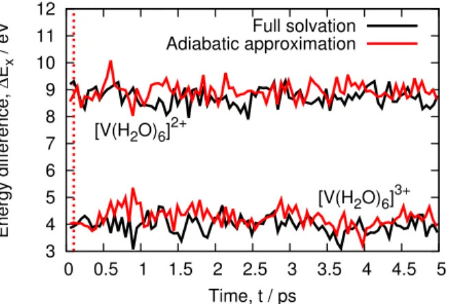
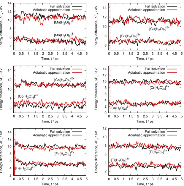
Following the procedure extensively described elsewhere,19we perform such sampling by produc-ing two 5 picosecond QM/MM NVT trajectories, one for each oxidation state, [M(H2O)6]3+ and [M(H2O)6]2+. As shown below for vanadium (Figure 3), the energy gap for both oxidation state exhibits a flat profile, meaning that our simulation seems converged within 5ps. Similar profiles for the other elements as well as computed averages are given in the Supporting Information. Snap-shots, on which energy calculations are carried out, are collected every 40 femtoseconds for both trajectories.
3
Results and discussion
This section is organized as follows. First, we validate our method by comparing quantities from the adiabatic approximation to the full solvation QM/MM scheme. Then, we compare our redox potentials with experimental values and discuss the predictive power of our method. Finally, we provide timings to evaluate the speed up brought by the adiabatic approximation.
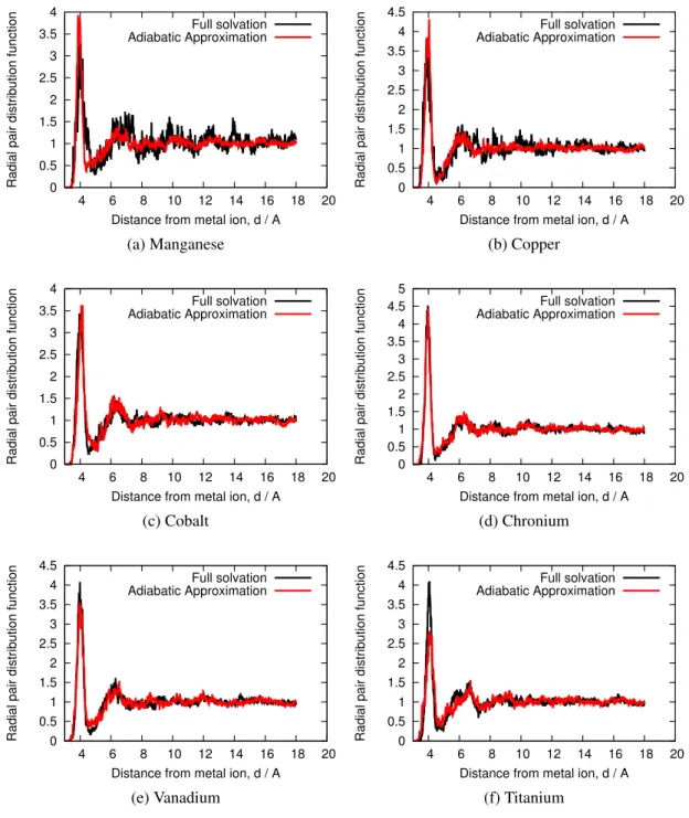
Figure 3 shows the fluctuations of the energy difference between the oxidized and reduced aqueous vanadium ions over 5 picoseconds. We observe that the observables have similar average and variations for both the reduced and oxidized states. For illustration purposes, we only show the vanadium data in Figure 3 but the same observation can be made for all other ions studied here (see Supporting Information). Consequently, it seems that the adiabatic approximation does not lead to deviations from the "true" ensemble for the present timescale. This is also supported by the metal-oxygen radial pair distribution functions (provided in the Supporting Information). Both methods give very similar distributions meaning that the adiabatic approximation gives a faithful representation of the solvent structure around the solute.
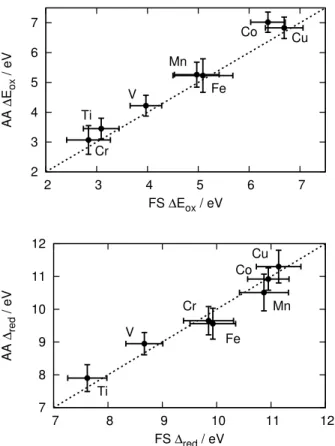
To better assess the discrepancies between the two QM/MM schemes, we look at the energy differences of the first row oxidized and reduced transition metal ions. Figure 4 gives the corre-lation plots of the adiabatic approximation quantities against the full solvation ones. We observe
3 4 5 6 7 8 9 10 11 12 0 0.5 1 1.5 2 2.5 3 3.5 4 4.5 5 Energy difference, ∆ Ex / eV Time, t / ps [V(H2O)6]3+ [V(H2O)6]2+ Full solvation Adiabatic approximation
Figure 3: Energy difference of vanadium aqueous ions across 5ps QM/MM trajectories. Both reduced (top curves) and oxidized (bottom curves) states are shown for both the full solvation and adiabatic approximation schemes. The red dotted line mark the time at which we fixed the density of the QM region.
that the adiabatic approximation tends to very slightly overestimate ∆Eox (linear fit of slope 1.06,
R2= 0.99), while accurately predicting ∆Ered (linear fit of slope 1, R2= 0.94). This is
surpris-ing because the oxidized species are less polarizable than their reduced counterpart and we would then expect the adiabatic approximation to perform better rather than worse. This suggests that this effect might be an artefact of the simulation where the excess charge lead to small numerical inaccuracies Nevertheless, aside from ∆Eox(Co), all values are identical within error.
Finally, we use these results to calculate the redox potential of each species according to Equa-tion 1 and check against experiments. We quote the experimental data from the CRC Handbook51 where the hydrogen electrode is used as a reference. In our calculations, we do not have such ref-erence so we shifted our potentials by a constant (6.1 V) to minimize the offset of the correlation line, while setting the slope to 1. The results are shown in Figure 5. The potential of the reference hydrogen electrode is 4.43 V52 which indicates that we suffer from a systematic error in our ab-solute potentials. We attribute this error to an overestimation of the energy of solvation due to the use of a non polarizable water force field. To test this hypothesis further, we calculated the redox potentials of vanadium, copper and chronium in the adiabatic approximation with two other non polarizable force fields, SPC and SPCE (see Supporting Information) and report values within our error bars, meaning that our systematic error is insensitive to the (non polarizable) water model.
2 3 4 5 6 7 2 3 4 5 6 7 AA ∆ Eox / eV FS ∆Eox / eV Ti Cr V Fe Mn Co Cu 7 8 9 10 11 12 7 8 9 10 11 12 AA ∆red / eV FS ∆red / eV Ti Cr V Fe Mn Co Cu
Figure 4: Correlation between the full solvation (FS) and adiabatic approximation (AA) electron affinities (top panel) and ionization potentials (bottom panel) of transition metal aqueous ions. The dotted line (y=x) serves as a guide for the eye and the error bars shown are one standard deviation.
This is consistent with the findings in reference19 where the theoretical full solvation redox poten-tials computed with a polarizable force field were shifted of 4.4 eV compared with experiments. Finally, we note that some of the systematic error observed in this study may also be attributed to the approximated long range electrostatics QM-MM interactions of the non periodic QM system.
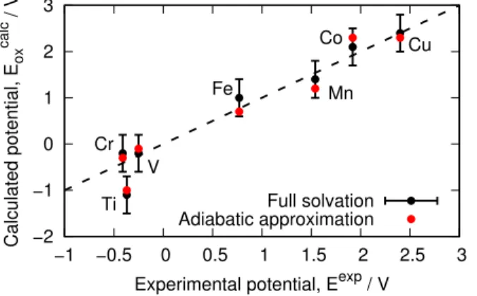
−2 −1 0 1 2 3 −1 −0.5 0 0.5 1 1.5 2 2.5 3 Ti Cr V Fe Mn Co Cu Calculated potential, E ox calc / V
Experimental potential, Eexp / V Full solvation Adiabatic approximation
Figure 5: Comparison of the calculated and experimental redox potential of transition metal aque-ous ions. The dotted line (y=x) serves as a guide for the eye and the error bars for the computed values are one standard deviation of the full solvation case (in black). The results for the adiabatic approximation scheme are shown on top of it (in red).
The agreement between calculated and measured redox is excellent for all ions but titanium. Nevertheless, since the calculated values are similar with both methods, the discrepancy is not due to the nature of our approximation. Rather, it appears to be a failure of QM/MM in general to capture the electronic properties of this specific ion. This is supported by earlier work19 on redox potentials of aqueous ions where QM/MM with polarizable force field equally fails to quantify the ability of titanium ions to gain electrons. Overall, QM/MM calculations accurately predict the redox properties of ions in water, unlike implicit solvent models which lack specific hydrogen bonding interactions.14,19
We report an adiabatic approximation theory-to-experiments RMSD of 0.32 V while the full solvation theory-to-experiments RMSD is 0.31V (the theory-to-theory root RMSD being 0.17 V). Therefore, our calculation scheme leads to results that are statistically very similar to conventional QM/MM calculations, largely improving on implicit solvent models (RMSD of 1.48 as reported in Ref19). This validates the adiabatic approximation method for the calculation of redox properties
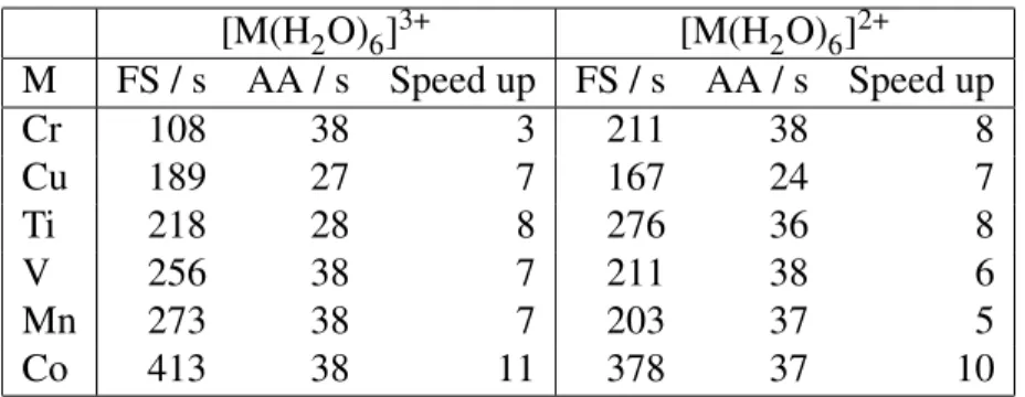
of ions in water, which is as accurate as the full solvation calculations while improving on the cost. Interestingly, this implies that the polarization of the solute (not accounted for within the adiabatic approximation) is of secondary significance here. Consequently, our findings suggest that redox potentials are dominated by solvent effects while changes du to solute polarization remain within the noise of our data. To quantify the speed up, we present the timings of our calculations (performed with CP2K) in Table 1.
Table 1: CP2K timings in seconds per NVT step for the full solvation (FS) and the adiabatic approximation (AA) QM/MM schemes. There are a total of 6442 atoms in all these calculations, including 19 QM atoms. [M(H2O)6]3+ [M(H2O)6]2+ M FS / s AA / s Speed up FS / s AA / s Speed up Cr 108 38 3 211 38 8 Cu 189 27 7 167 24 7 Ti 218 28 8 276 36 8 V 256 38 7 211 38 6 Mn 273 38 7 203 37 5 Co 413 38 11 378 37 10
Up to a factor 10 is gained per step of QM/MM simulations. This is due to the fact that only one SCF step is required as opposed to tens in the full solvation scheme. This represents valuable savings that would allow to produce trajectories of bigger systems and/or for a longer time. We note that, at present, the implementation of the fixed electron density is done without any changes to the CP2K code. Instead, we bypass the SCF cycle by setting trivially reachable convergence threshold. This means that the matrix representing the QM/MM hamiltonian is built and diagonalized each time. More savings could be achieved if we could execute only the calculation of the interaction of the QM density with the MM charges at each step. Moreover, while the original timings depend on the nature and the charge of the QM region, the adiabatic approximation scheme provides a more consistent cost for each transition metal atoms across the periodic table. This is explained by the fact that the limiting step in the adiabatic approximation scheme is the calculation of the QM/MM interaction, which scales with the size of the MM region. In our test systems, we used a significant number of water molecules that, if reduced, would also improved on the savings. The tuning of the
implementation of the adiabatic approximation in explicit solvent models and the size of the MM region is to be considered on a case-to-case basis. Overall, by using the same separation of degrees of freedom as in implicit solvent models, we bring QM/MM simulations one step closer to the cost of a PCM calculation while retaining the high-accuracy of solvent configurational sampling. For example, a PCM calculation costs about the same as one SCF step, so 400 seconds here, for cobalt ions (see Table 1). A QM/MM calculation requires 10 000 steps (5ps trajectories) for a total cost of 4 millions of seconds for the full solvation and only 400 000 seconds for the adiabatic approximation scheme. Therefore, this approach could be used to calculate the redox properties of solvated systems for which implicit solvent models fail without dramatically increasing the cost.
4
Conclusions
In this paper, we exploited the approximate separation of the degrees of freedom between a solute (QM region) and a solvent (MM region) to produce QM/MM NVT trajectories at lower compu-tational cost. We assumed that the solute can be represented by a single electron density (as it is the case in implicit solvent models) while preserving the configurational sampling of the MM wa-ter molecules. We tested this method by calculating the redox potential of transition metal ions in water and comparing it with conventional QM/MM calculations. The two procedures are character-ized by a RMSD of 0.17 V on the systems studied here, meaning that the adiabatic approximation works well for aqueous ions. However, this study focuses on the calculation of redox potential of simple transition metal ions in water. Although it works surprisingly well in this context, the extension of our results to other properties and solvents would require further testing, which is outside the scope of this paper.
In the future, we would broaden the range of our study cases and evaluate the validity of the adiabatic approximation in explicit solvent models for systems where implicit solvent models are found to give erroneous results. This is the case for biological systems for example where hy-drophobic effects and hydrogen bonding makes the configurational sampling of the environment
crucial. Often too large to be treated by conventional QM/MM, we expect the adiabatic approxima-tion scheme to bring a promising alternative. Furthermore, we could use implicit solvent models to guess the electron density of the solute to fix, discarding all steps of full solvation QM/MM cal-culations. The adiabatic approximation would then be a correction to these much cheaper models that incorporate the heterogeneity of the surrounding medium.
Finally, more savings on the computational cost could be achieved by discarding the building and diagonalization of the QM/MM hamiltonian at each step. Rather, we would develop a way to, once the electron density of the solute is found, only calculate the interaction term with the MM charges at each step.
Acknowledgement
This work was funded by NSF Grant No. CHE-1058219. We thank Florian Schiffman and Vedran Miletic for their help with the CP2K software package.
Supporting Information Available
This material is available free of charge via the Internet at http://pubs.acs.org/.
Notes and References
(1) Kirschner, K. N.; Woods, R. J. Proc. Natl. Acad. Sci. U.S.A. 2001, 98, 10541–10545. (2) Zagrovic, B.; Vijay, P. J. Comput. Chem. 2003, 24, 1432–1436.
(3) Sundararajan, M.; Hillier, I. H.; Burton, N. A. J. Phys. Chem. A 2006, 110, 785–790.
(4) Bhattacharyya, S.; Stankovich, M. T.; G., T. D.; Gao, J. J. Phys. Chem. A 2007, 111, 5729– 5742.
(5) Tuckerman, J. T.; Polyansky, D. E.; Wada, T.; Tanaka, K.; Fujita, E. Inorg. Chem. 2008, 47, 1787–1802.
4 6 8 10 12 14 0 0.5 1 1.5 2 2.5 3 3.5 4 4.5 5 Energy difference, ∆ Ex / eV Time, t / ps [Mn(H2O)6]3+ [Mn(H2O)6]2+ Full solvation Adiabatic approximation 6 8 10 12 14 0 0.5 1 1.5 2 2.5 3 3.5 4 4.5 5 Energy difference, ∆ Ex / eV Time, t / ps [Cu(H2O)6]3+ [Cu(H2O)6]2+ Full solvation Adiabatic approximation 6 8 10 12 14 0 0.5 1 1.5 2 2.5 3 3.5 4 4.5 5 Energy difference, ∆ Ex / eV Time, t / ps [Co(H2O)6]3+ [Co(H2O)6]2+ Full solvation Adiabatic approximation 0 2 4 6 8 10 12 14 0 0.5 1 1.5 2 2.5 3 3.5 4 4.5 5 Energy difference, ∆ Ex / eV Time, t / ps [Cr(H2O)6]3+ [Cr(H2O)6]2+ Full solvation Adiabatic approximation 2 4 6 8 10 12 14 0 0.5 1 1.5 2 2.5 3 3.5 4 4.5 5 Energy difference, ∆ Ex / eV Time, t / ps [Fe(H2O)6]3+ [Fe(H2O)6]2+ Full solvation Adiabatic approximation 2 4 6 8 10 12 0 0.5 1 1.5 2 2.5 3 3.5 4 4.5 5 Energy difference, ∆ Ex / eV Time, t / ps [Ti(H2O)6]3+ [Ti(H2O)6]2+ Full solvation Adiabatic approximation
Figure 6: Energy difference of the aqueous ions across 5ps QM/MM trajectories. Both reduced (top curves) and oxidized (bottom curves) states are shown for both the full solvation and adiabatic approximation schemes. The red dotted line mark the time at which we fixed the density of the QM region.
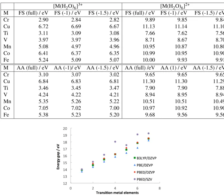
Table 2: Computed averages of the energy differences of both oxidation state of the transition metal ions studied in this work. We compare the average over the entire trajectory (full) to the averages excluding the first 1 (-1) and 1.5 (-1.5) ps to show that our observables are converged within our simulated timescale. [M(H2O)6]3+ [M(H2O)6]2+ M FS (full) / eV FS (-1) / eV FS (-1.5) / eV FS (full) / eV FS (-1) / eV FS (-1.5) / eV Cr 2.90 2.84 2.82 9.89 9.85 9.84 Cu 6.72 6.69 6.67 11.13 11.14 11.10 Ti 3.11 3.09 3.08 7.66 7.62 7.56 V 3.97 3.97 3.96 8.71 8.67 8.70 Mn 5.08 4.97 4.96 10.95 10.87 10.80 Co 6.41 6.37 6.35 10.99 10.95 10.90 Fe 5.24 5.09 5.07 10.00 9.93 9.91
M AA (full) / eV AA (-1)/ eV AA (-1.5) / eV AA (full) /eV AA (1) / eV AA (-1.5) / eV
Cr 3.10 3.07 3.02 9.65 9.65 9.65 Cu 6.84 6.83 6.81 11.30 11.30 11.29 Ti 3.46 3.45 3.47 7.90 7.90 7.88 V 4.24 4.22 4.21 8.94 8.95 8.94 Mn 5.35 5.26 5.22 10.51 10.51 10.49 Co 7.05 7.02 7.00 10.97 10.92 10.90 Fe 5.38 5.23 5.20 9.68 9.56 9.56
Figure 7: Comparison of PBE0 and PBE with B3LYP on the calculation of the energy difference of the hydrated metal ions (QM calculation on the solute). As expected PBE0 gives a very similar trend than B3LYP while PBE underestimates the energy gap by a varying amount across the series, making it a less accurate method for this study. Also shown the poor performance of the SZV basis set to emphasize the need for a polarized basis set.
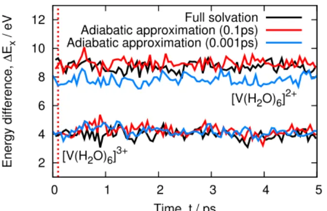
Table 3: Computed averages of the data shown in Figure 8. FS / eV AA (0.1ps) / eV AA (0.001ps) / eV [V(H2O)6]3+ 3.97 4.24 4.19
2 4 6 8 10 12 0 1 2 3 4 5 Energy difference, ∆ Ex / eV Time, t / ps [V(H2O)6]3+ [V(H2O)6]2+ Full solvation Adiabatic approximation (0.1ps) Adiabatic approximation (0.001ps)
Figure 8: Energy difference of vanadium aqueous ions across 5ps QM/MM trajectories. We com-pare the adiabatic approximation made from 0.01ps (red) to the adiabatic approximation made form 0.001ps (blue). When compared with the full solvation (black) we see that the adiabatic approximation from 0.001ps adequately captures the energy gap of the V3+ ions while underesti-mating the energy gap of the V2+ ions. This leads to an underestimation of the redox potential of 0.22eV (see Table 3 that falls within the error of this study (about 0.3 eV).
−2 −1 0 1 2 3 −1 −0.5 0 0.5 1 1.5 2 2.5 3 Ti Cr V Fe Mn Co Cu Calculated potential, E ox calc / V
Experimental potential, Eexp / V FS TIP3P AA TIP3P AA SPCE AA SPC
Figure 9: Comparison of the calculated and experimental redox potential of transition metal aque-ous ions. Here, we add the data corresponding to the SPCE (in green) and SPC (in blue) force field to the data presented in Figure 5. We observe that the results are insensitive to the force field, as mentioned in the main text.
0 0.5 1 1.5 2 2.5 3 3.5 4 4 6 8 10 12 14 16 18 20
Radial pair distribution function
Distance from metal ion, d / A Full solvation Adiabatic Approximation (a) Manganese 0 0.5 1 1.5 2 2.5 3 3.5 4 4.5 4 6 8 10 12 14 16 18 20
Radial pair distribution function
Distance from metal ion, d / A Full solvation Adiabatic Approximation (b) Copper 0 0.5 1 1.5 2 2.5 3 3.5 4 4 6 8 10 12 14 16 18 20
Radial pair distribution function
Distance from metal ion, d / A Full solvation Adiabatic Approximation (c) Cobalt 0 0.5 1 1.5 2 2.5 3 3.5 4 4.5 5 4 6 8 10 12 14 16 18 20
Radial pair distribution function
Distance from metal ion, d / A Full solvation Adiabatic Approximation (d) Chronium 0 0.5 1 1.5 2 2.5 3 3.5 4 4.5 4 6 8 10 12 14 16 18 20
Radial pair distribution function
Distance from metal ion, d / A Full solvation Adiabatic Approximation (e) Vanadium 0 0.5 1 1.5 2 2.5 3 3.5 4 4.5 4 6 8 10 12 14 16 18 20
Radial pair distribution function
Distance from metal ion, d / A Full solvation Adiabatic Approximation
(f) Titanium
Figure 10: Radial metal-oxygen distribution function for the series of transition elements studied here. In each case we compare the full solvation, in black to the adiabatic approximation, in red. For all the elements presented the radial pair distribution function from the adiabatic approxima-tion is extremely similar to the one from the full solvaapproxima-tion scheme, meaning that the adiabatic approximation gives a faithful representation of the solvent structure around the solute.
(6) Gao, J.; Truhlar, D. G. Annu. Rev. Phys. Chem. 2002, 53, 467–505. (7) Gao, J.; Xia, X. Science 1992, 258, 631–635.
(8) Vaissier, V.; Barnes, P.; Kirkpatrick, J.; Nelson, J. Phys. Chem. Chem. Phys. 2013, 15, 4804– 4814.
(9) Duarte, F.; Amrein, B. A.; Blaha-Nelson, D.; Kamerlin, S. C. L. Biochim. Biophys. Acta. 2015, 1850, 954–965.
(10) Fromaneck, M. S.; Li, G.; Zhang, X.; Cui, Q. J. Theo. Comp. Chem. 2002, 1, 53–67. (11) Zeng, X.; Hu, H.; Cohen, A. J.; Yang, W. J. Chem. Phys. 2008, 128, 124510.
(12) Li, G.; Zhang, X.; Cui, Q. J. Phys. Chem. B 2003, 107, 8643–8653. (13) Blumberger, J. Chem. Rev. 2015, 115, 11191–11238.
(14) Tomasi, J.; Mennucci, B.; Cammi, R. Chem. Rev. 2005, 105, 2999–3093. (15) Barone, V.; Cossi, M. J. Phys. Chem. A 1998, 102, 1995–2001.
(16) Klamt, A.; Schuurmann, G. J. Chem. Soc., Perkin Trans 1993, 2, 799–805. (17) Cances, E.; Mennucci, B.; Tomasi, J. J. Phys. Chem. 1997, 107, 3032–3041. (18) Eisenberg, D.; Mclachlan, A. D. Nature 1986, 319, 199–203.
(19) Wang, L.-P.; Van Voorhis, T. J. Chem. Theory Comput. 2012, 8, 610–617.
(20) Artacho, E.; Sanchez-Portal, D.; Ordejon, P.; Garcia, A.; Soler, J. M. phys. stat. sol. (b) 1999, 215, 809–817.
(21) Laino, T.; Mohamed, F.; Laio, A.; Parrinello, M. J. Chem. Theory Comput. 2006, 2, 1370– 1378.
(23) Gao, J.; Truhlar, D. G. Annu. Rev. Phys. Chem. 2002, 53, 467–505.
(24) Zeng, X.; Hu, H.; Hu, X.; Cohen, A. J.; Weitao, Y. J. Chem. Phys. 2008, 128, 124510. (25) Field, M. J.; Bash, P. A.; Karplus, M. J. Comput. Chem. 1990, 11, 700–733.
(26) Gao, J.; Amara, P.; Alhambra, C.; Field, M. J. J. Phys. Chem. 1998, 102, 4714–4721.
(27) Hutter, J.; Iannuzzi, M.; Schiffmann, F.; VandeVondele, J. WIREs Comput. Mol. Sci. 2014, 4, 15–25.
(28) Blumberger, J. Phys. Chem. Chem. Phys. 2008, 10, 5651–5667.
(29) Olsson, M. H. M.; Hong, G.; Warshel, A. J. Am. Chem. Soc 2003, 125, 5025–5039. (30) Wesolowski, T. A.; Warshel, A. J. Phys. Chem. 1993, 97, 8050–8053.
(31) Bentzien, J.; Muller, R. P.; Florian, J.; Warshel, A. J. Phys. Chem. B 1998, 102, 2293–2301. (32) Amadei, A.; Daidone, I.; Aschi, M. Phys. Chem. Chem. Phys. 2012, 14, 1360–1370.
(33) Amadei, A.; Daidone, I.; Bortolotti, C. A. RSC Adv. 2013, 3, 19657–19665.
(34) Mueller, R.; North, M.; Yang, C.; Hati, S.; Bhattacharyya, S. J. Phys. Chem. B 2011, 115, 3632–3641.
(35) Woiczikowski, P. B.; Steinbrecher, T.; Kubar, T.; Elstner, M. J. Phys. Chem. B 2011, 115, 9846–9863.
(36) Chandler, D.; Andersen, H. C. J. Chem. Phys. 1972, 57, 1930–1937. (37) Yang, X.; Baik, M.-H. J. Am. Chem. Soc. 2004, 126, 13222–13223. (38) L.-P., W.; Wu, Q.; Van Voorhis, T. Inorg. Chem. 2010, 49, 4543–4553. (39) Nam, K.; Gao, J.; York, D. M. J. Chem. Theory Comput. 2005, 1, 2–13.
(40) Jin, H.; Goyal, P.; Kumar Das, A.; Gaus, M.; Meuwly, M.; Cui, Q. J. Phys. Chem. B 2016, 120, 1894–1910.
(41) Ref. 40, and references therein.
(42) Mohammed, A. M. Bull. Chem. Soc. Ethiop. 2010, 24, 239–250.
(43) O’Brien, J. T.; Williams, E. R. J. Phys. Chem. A 2011, 115, 14612–14619. (44) Shao, Y. e. a. Mol. Phys. 2015, 113, 184–215.
(45) Becke, A. D. J. Chem. Phys. 1993, 98, 5648–5652.
(46) Hay, P. J.; Wadt, W. R. J. Chem. Phys. 1985, 82, 299–310.
(47) Jorgensen, W. L.; Chandrasekhar, J.; Madura, J. D.; Impey, R. W.; Klein, M. L. J. Chem. Phys.1983, 79, 926–935.
(48) VandeVondele, J.; Hutter, J. J. Chem. Phys. 2007, 127, 114105.
(49) Laio, A.; VandeVondele, J.; Rothlisberger, U. J. Chem. Phys. 2002, 116, 6941–6947.
(50) lain, T.; Mohammed, F.; Laio, A.; Parrinello, M. J. Chem. Theory Comput. 2005, 1, 1176– 1184.
(51) CRC Handbook of Chemistry and Physics, 91st ed; CRC Press: Boca Raton, FL2010, 2010. (52) Reiss, H.; Heller, A. J. Phys. Chem. 1985, 89, 4207–4213.