The Determinants Of Foreign Direct Investment In North African Countries Econometric Study With Panel Data

The determinants of foreign direct investment in North

African countries Econometric study with panel data

Dr. Mohamed RETIA  Dr. Khemissi GAIDI  Abstract:

Most countries in the world are working hard to attract more foreign direct investment. This paper aims to respond to the following question: what are the determinants determines of foreign direct investment in North African countries? The study employed panel data analysis: pooled ordinary least square method, fixed effects and Random Effect methods. As well as a dynamic panel model, ten countries were sampled for the study. The analyzed data covered for the period 19 -201 . And present a set of Stata11 programs to conveniently execute them.

The results indicate a significant long-run impact of trade openness; economic growth, inflation, and lag of FDI are considered as the most significant determinants of foreign direct investment inflows to North African countries.

Key words: FDI, fixed effect, Random Effect, Poold Mean Group (PMG)

and Mean Group (MG).

: نا ه و ا ا ر ة أ ا : ا لا ا ا إ ا ف ،ر ا ا و ، و لا ا ا و ؟ إ ل لود ا ا ر ا تاد رد ا ا ت إ ا ل جذ ا تا ا ، ا او جذ ا د ا إ ا ن ر ا ،

ـــــــــــــــــــــــــــــــــــــــ

 _{Associate Professor, University of Medea.}

ة ا ة نا ة 1980 -2010 ا ذو ، 11 stata أ ت ا ر او جذ ا ا ،ير ا ح ا ى ا ي ا ا إ أ ي ا ا ا ر ا ا و ا ،يد ا إ ل نا إ ا ا ر ا ا تاد ا : ت ، ا ا ا ، ا ا ، ا ا ر ا و ا ت ا ) PMG ) ت ا وو( MG ( 1. Introduction

Foreign direct investment (FDI) became an increasingly important element in global economic development and integration in recent years. This development occurred contemporaneously with the process of transition from socialism to capitalism and the integration of the Central and Eastern European countries (CEEC) into the world economy through trade and capital flows, as Di Mauro (1999) and Buch et al. (2003) discuss. FDI into transition economies may facilitate growth, promote technical innovation, and accelerate enterprise restructuring in addition to providing capital account relief (EBRD, 2002).

The objective of this article is to estimate-based on panel data- the main determinants

of FDI in North African countries. As shall be seen, factors such as the size and rate of growth

of the GDP, the availability of trade openness, the receptivity of foreign capital, the country risk rating, and the behavior of the stock market play important roles in FDI.

Our study is structured as follows: in Section 2 we have provided a definition and types of the determinants of direct foreign investment. In Section 3, we have examined recent studies that analyze the relation between FDI and several economic factors. In section 4, we have outlined our model and the hypotheses to be tested, and present the results obtained. The results are then analysed. In. lastly, in Section 5, we have

presented the conclusions of our study.

2. Definition and Types of FDI

The International Monetary Fund (1993) defines FDI as a category of international investment that reflects the objectives of a resident in one economy (the direct investor or source economy) obtaining a lasting interest in an enterprise resident in another economy (the direct investment enterprise or host economy). The lasting interest implies the existence of a long-term relationship between the direct investor and the direct investment enterprise, and a significant degree of influence by the investor on the management of the enterprise. FDI comprises (includes) not only mergers, take overs/acquisitions (brown field investments) and

new investments (green field investment), but also reinvested earnings and loans and similar capital transfers between parents and affiliates.1

3. Determinants of FDIs: empirical studies

Empirical studies that attempt to estimate the importance of the different determinants of FDI concentrate more on attraction factors, i.e., locational factors, since available data make it difficult to identify which countries the investments come from, unless a large set of countries and years is analysed. The capital propriety advantages, the degree of openness of the economy, as well as several other institutional variables, as shall be seen. However, the relation between FDI and economic growth deserves special attention. If, on one hand, economic growth is a powerful stimulant to the inflow of FDI, on the other hand, an increase in foreign investment –since this would mean an increase in the existing capital stock (green field investment) – would be also one of the factors responsible for economic growth, meaning the existence of an

ـــــــــــــــــــــــــــــــــــــــ

1Sutana Thanyakhan (2008), the Determinants of FDI and FPI in Thailand: a Gravity Model Analysis, a Thesis submitted in partial fulfillment of the requirements for the Degree of Doctor of Philosophy in Economics Lincoln University 2008.

endogeneity problem. There are, also, other studies that deal with proving the relation between FDI and the level of economic activity.

The next set of studies examined deals with FDI in developing countries, Nunnenkamp and Spatz1, studying a sample of 28 developing countries during the period of 1987-2000, find significant Spearman correlations between FDI flows and per capita GNP, risk factors, years of schooling, foreign trade restrictions, complementary production factors, administrative bottlenecks2 and cost factors3. Population, GNP growth, firm entry restrictions, post-entry restrictions, and technology regulation all proved to be non significant.

However, when regressions were performed separately for the non-traditional factors, in which traditional factors were controls (population and per capita GNP), only factor costs produced significant results and, even so, only for the 1997-2000 period. Holland and others (2000) reviewed several studies for Eastern and Central Europe, producing evidence of the importance of market size and growth potential as determinants of FDI. Tsai (1994) analysed the decades of 1970 and 1980 and addressed the endogeneity problem between FDI and growth by developing a system of simultaneous equations.

Campos and Kinoshita (2003) use panel data to analyze 25 transition economies between 1990 and 1998. They reached the conclusion that for said set of countries FDI is influenced by economy clusters, market size, the low cost of labor, and abundant natural resources. Besides all these factors, the following variables presented significant results:

sound institutions, trade openness, and lower restrictions to FDI inflows. Garibaldi and others (2001), based on a dynamic panel of 26 transition economies between 1990 and 1999, analyzed a large set of

ـــــــــــــــــــــــــــــــــــــــ

1 Nunnenkamp Peter & Spatz Julius (2002), Determinants of FDI in Developing Countries: has Globalization Changed the Rules of the Game? Transnational Corporations, vol 11 (2).

variables that were divided into macroeconomic factors, structural reforms, institutional and legal frameworks, initial conditions, and risk analyses. The results indicated that macroeconomic variables, such as market size, fiscal deficit, inflation and exchange regime, risk analysis, economic reforms, trade openness, availability of natural resources, barriers to investment and bureaucracy all had the expected signs and were significant.

Loree and Guisinger (1995) studying the determinants of foreign direct investment by the United States in 1977 and 1982 (both towards developed countries as well as toward developing countries), concluded that variables related to host country policy were significant in developed countries only when infrastructure was an important determinant in all regions.

The several results obtained by Lipsey (2000) allows us to infer that the effect of FDI on growth is positive, but reduced, and depends strongly on the interaction with the level of schooling in the host country. Soto (2000), working with panel data for developing countries for the 1986-97 period, concluded that FDI contributes positively to growth through the accumulation of capital and the transfer of technology.

Lastly, Buckley and others (2002) used panel data for several regions in China for the 1989-98 period. In the first place, the author points out that if the rate of growth of FDI has positive effect upon GDP growth, the reverse does not hold true. Secondly, no evidence was found to support the hypothesis according to which the efficiency of FDI depends on a level of human capital. Contrastingly, human capital is more significant in less developed provinces, while FDI stimulates growth notably in the more developed provinces.1

ـــــــــــــــــــــــــــــــــــــــ

1 Marcelo Braga Nonnemberg, Mario Jorge Cardoso de Mendonça (2001), the determinants of foreign direct investment in developing countries, Brazil. p5-6.

4. The Model Specifications and Estimation Framework:

Any panel data would involve i=1,…..,N and t=1,…..,T, where i represents the number of countries and t represents the period of data studied. In the estimation process of the paneldata, there will be four critical assumptions of panel analysis with respect to the degree of homogeneity (same, without changing) across panels.

By relaxing each assumption, it will increase the degree of accuracy nearer to the real world. This is especially true, since the allowance for

the heterogeneity effects (in the estimation cross panels} will accommodate the differences and uniqueness operations for each economy (the reality). Here, we will show how the relaxation for these assumptions, through the Fixed Effect (FE) model, Random Effect(RE), pool mean group PMG) and mean group (MG) estimator. From the literature, we can show that the general function that

explains the fdi of is a factor as below:

From the above model, the long run model for the panel illustrated is as follows: Lfdiit = μi + βtXit + εit ………….(2)

Where i represent cross-sections data i=1,2,..,10, and t represents number of periods t= 1,2,...,31 years from 1980 to 2010.Xit is the vector

of explanatory variable( regressors) If the variables are I(1) and cointegrated, then the stationary term is I(0) for all panels.

Where:

 Lfdi :The dependent variable is the logarithm of foreign direct investment as a share of nominal GDP

 Lgdp: log level of GDP per capita

 Lopen: the degree of trade openness: Computed as a ratio of the total exports of goods and services to GDP.

 Lsk: Logarithm of physical capital stock  Lkh: Logarith of human capital stock  Lpop: the logarithm of Population growth.  Linf: Logarithm inflation rate

4.1 Fixed Effect (FE) and Random Effect (RE) Model

There are two common assumptions made about the individual specific effect, the random effects assumption and the fixed effects assumption. The random effects assumption (made in a random effects model) is that the individual specific effects are uncorrelated with the independent variables. The fixed effect assumption is that the individual specific effect is correlated with the independent variables. If the random effects assumption holds, the random effects model is more efficient than the fixed effects model. However, if this assumption does not hold, the random effects model is not consistent.

In panel data analysis, the term fixed effects estimator (also known as the within estimator) is used to refer to an estimator for the coefficients in the regression model. If we assume fixed effects, we impose time independent effects for each entity that are possibly correlated with the regressors. 1

4.1.1 Estimation Results

A number of different specifications of the model are estimated using

the panel data of 10 countries for the period 1980 to 2010. (Data extracted from World Bank 2014).The following table shows the

results of the estimation of the three Panel models (homogeneous model, fixed effectand random effect).

ـــــــــــــــــــــــــــــــــــــــ

1 Baltagi, Badi H.(2001), Econometric Analysis of Panel Data, 2nd edition. New York: John Wiley &Sons, LTD.

Table1: estimation results of static panel (pooled,fe,re)

Source: stata 14

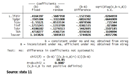
The model has a standard panel with T being larger than N and the results for the three models are reported in Table1. Columns 2 and 3 of Table 1 present static RE and FE panel data models, In order to check whether the FE model is appropriate or not, we performed a Hausman type test of no correlation between μi with the regressors. The test returned a χ2 value of 18.85 with a p-value of 0.0087, which means that the FE model is the preferred one. As shown in Table 3

 Testing for random effects: Breusch-Pagan Lagrange multiplier

(LM) : The estimates of the pooled model and the random effects model are reported in Table 2.

Table 2: Breusch and Pagan Lagrangian Multiplier Test.

Source: stata11

To account for the panel nature of the data, in the pooled model the t statistics are computed using an estimated covariance matrix of the estimated coefficients that is corrected for clustering. The comput-ed value of the LM test is 1.95 (0.1625) which clearly accept the null hypothesis of random effects (p-value) in brackets. and therefore the appropriate model is the individual random effects model.

 Hausman test: To distinguish between RE and FE, you will want

to do a Hausman test. The BP test does not help with this decision. This test is shown in the following table

Table 3: Hausman test

The Hausman test indicates the presence of a correlation between the individual component and the regressors.

The FE model is also known as the least squares dummy variables. As the name suggest, it requires inclusion of dummy variables as a tool, to detect variation in the intercept across units. FE model imposes most restrictive constraints (towards the homogeneity) to all four assumptions except the intercept for each cross section.

4.1.2 Estimation of the fixed effects models

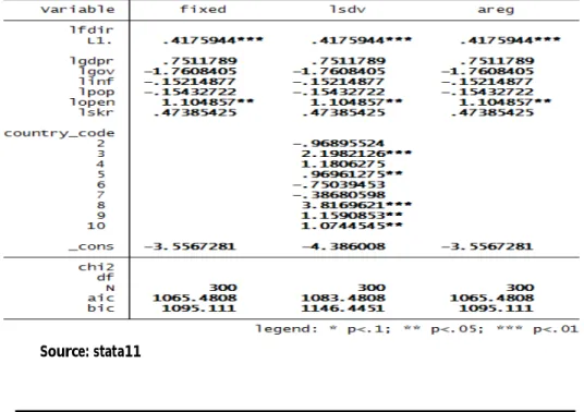
If we are concerned that the OLS results may be biased because of unobserved heterogeneity then we need to try and account for this One way of doing this is to create 10 dummy variables individual-specific dummy variables - one for each individual in the data to proxy for time invariant individual unobserved effect, In this case we use the estimation method (LSDV), The results of estimation of the fixed effects models are shown in Table 4 .

Table 4 : estimation of the fixed effects models (lfdi : dependent

variable)

The results of the estimation of the model for the fixed effects of the North African countries listed in the table above show that:

- The statistical value of Fisher's F test indicates a statistical significance of the model Although most of the parameters of the variables were insignificant except for the logarithm of trade openness. and the logarithm of the lagged FDI

- The lagged FDI variable lFDIt-1 produces a significant positive coefficient, indicating that foreign firms tend to concentrate their activities at the location where other foreign firms are already located, and thus, it supports the agglomeration effects.

4.2 Dynamic Panel Models

4.2.1 Panel unit root tests and cointegration

Engle and Granger [1987] argue that the direct application of OLS or GLS to non-stationary data produces regressions that are mis specified or spurious in nature. These regressions tend to produce performance statistics that are inflated in nature, such as high R2's and t-statistics, which often lead investigators to commit a high frequency of Type I errors [Granger and New bold, 1974].

In recent years, a number of investigators, notably Levin, Lin and Chu (2002), Breitung (2000), Hadri (1999), and Im, Pesaran an Shin (2003), have developed panel-based unit root tests that are similar to tests carried out on a single series. Interestingly, these investigators have shown that panel unit root tests are more powerful (less likely to commit a Type II error) than unit root tests applied to individual series because the information in the time series is enhanced by that contained in the cross-section data. In addition, in contrast to individual unit root tests which have complicated limiting distributions, panel unit root tests lead

to statistics with a normal distribution in the limit 1.

With the exception of the IPS test, all of the aforementioned tests assume that there is a common (identical) unit root process across the relevant cross-sections (referred to in the literature as pooling the residuals along the within-dimension).(Miguel D. Ramirezt(2006)),The LLC and Breitung tests employ a null hypothesis of a unit root using the following basic Augmented Dickey Fuller (ADF) specification:

Δy_it = αy_it-1 +Σβ_ijΔy_it-j + X_itδ + ν_it (3)

Where yit refers to the pooled variable, Xit’ represents exogenous variables in the model such as country fixed effects and individual time trends, and νit refers to the error terms which are assumed to be mutually independent disturbances.

The result shows that at 5% level of significance we accept null hypothesis that means the series are not stationary. Except foreign direct investment which was stationnary at the level. After taking the first difference at 5% level of significance we reject null hypothesis, so first difference of the series is stationary. According to these results, the best method to be used in the analysis is the Panel-ARDL model, which allows this diversity in the orders of integration of variables.

Using Pedroni, Kao and Johansen Fisher panel cointegration test for three different opportunity cost, the test result give strong evidence that the variables has long run equilibrium.

4.3 Poold Mean Group (PMG) and Mean Group (MG)

PMG technique is pooling the long run parameters while avoiding the inconsistency problem flowing from the heterogeneous short run dynamic relationships. Plus, the PMG relax the restriction on the common coefficient of short run while maintain the assumption on the

ـــــــــــــــــــــــــــــــــــــــ

1Baltagi, Badi H. (2001) , “Econometric Analysis of Panel Data”, 2nd edition. New York: John Wiley &Sons, LTD.

homogeneity of long run slope. The estimation of the PMG requires reparameterization into error correction system.

 The model:

Suppose that given data on time periods, t=1,2,…,T, and groups, i=1,2,…,N, we wish to estimate an ARDL model:

 

4 ... ... u x fdi fdi _{i,t j i it} q 0 j ij j t , i p 1 j ij it           





It where xit is the vector of explanatory variable( regressors) for group I, ui represent the fixed effects, the coefficients of the lagged dependent variables,

ij

 , are scalars, andij are k1coefficient vectors. T

must be large enough such that we can estimate the model for each group separately. For notational convenience we shall use a common T and p across groups and a common q across group and regressors, but this is not necessary. Similarly, time trends or other types of fixed regressors such as seasonal dummies can be included in (4) .but to keep the notation simple we do note allow for such effects. It is convenient to work with the following re-parameterization of (4).

 

1 ,... 2 , 1 , , 1 ,..., 2 , 1 , , ), 1 ( , ,..., 2 , 1 , ,... 2 , 1 5 .. ... ... 1 1 * 0 1 , 1 0 * , 1 1 1 ,                         













              q j and p j T t and N i u x fdi x fdi fdi q j m im p j m ij im ij q j ij i p j ij i it i j t i q j ij j t i p j it i t i i it ij             

If we stack the time-series observations for each group, equation (5) can be written as1

 

6 ... * , 1 0 , 1 1 1 , i j ij i it q j j i p j i i i i i y X fdi X u fdi     _ij        _       





, N ,... 2 , 1

i  where y_i



fdi_i1,fdi_i2,...,fdi_iT



T1Vector of the

observations on the dependent variable of the i-th group,X_i 



x_i1,x_i2,...,x_iT



 is the matrix of observations on the







 1,...,1

 a T1Vector of ones, y_i,jand X_i,j are j period lagged

values of yi and Xi , yi  yi  yi,1,Xi  Xi  Xi,1 , yi,j and j

i

X





, are j period lagged values of yi and Xi , and



₁,..,



.  _{i iT}

i  



The PMG estimator is an intermediate estimator which allows the intercepts, short-run coefficients, and error variances to be different across groups, but the long-run coefficients are constrained to be homogeneous. There are good reasons to believe that the long-run equilibrium relationship amongst variables should be identical across groups, while the short-run dynamics are heterogeneous. This dynamic estimator is more likely to capture the true nature of the data .1

We Assume the long-run growth relationship is given by:

 

T t N i u l lpop lopen lsk dpr lfdi_{it i i it i it i it i it i it it} ,..., 2 , 1 , ,..., 2 , 1 7 .. inf lg _{2 3 4 5} 1 0                 

where FDIit is the foreign direct investement, gdprit is real GDP per capita growth rate, sk is the Capital stock, pop is the population, open represent the trade openness and inf is the rate of inflation.

We Assume that all of these variables are I(1) and cointegrated. This means uit is an I(0) process for all i and is independently distributed across t. They are also assumed to be distributed independently of the regressors. Suppose the maximum lag of every variable is one, the autoregressive distributed lag, ARDL (1, 1, 1, 1, 1, 1), model

 

8

...

inf

inf

lg

lg

1 , , 51 50 , 41 40 1 , 31 30 1 , 21 20 1 , 11 10 it t i i j t i i it i j t i i it i t i i it i t i i it i t i i it i i it

lfdir

l

l

lpop

lpop

lopen

lopen

lsk

lsk

dpr

dpr

u

lfdi



















































     

ـــــــــــــــــــــــــــــــــــــــ

1 Kang Yong Tan (2006),“A pooled mean group analysis on aid and growth” University of Oxford, p4.

4.3.1 Estimation Results

Table (5) presents results obtained from alternative estimators: MG, PMG. The PMG computations were obtained using the Newton-Raphson algorithm without a common time trend. The constraint of common long-run coefficients (i.e. from MG to PMG) has yielded lower standard errors and slower speed of adjustment. This outcome is expected given that the MG estimators are known to be inefficient. The result reveals that economic growth and trade openness and Population growth are significant and contribute positively to FDI in the long-run. However, inflation reduces the long-run FDI.

Being an ARDL model, the result may be sensitive to the choice of lag length. In what follows, I impose a maximum lag length of one for the Akaike Information Criterion (AIC) and the Schwarz Bayesian Criterion to obtain optimal lag length for various variables. The negative result of aid reducing growth when coupled with .good. policy is found to be robust. The Hausman test statistic confirms that the long-run homogene-ous coefficient restrictions can not be rejected at the 1% significance level. This indicates the presence of a long-run homogeneous relationship amongst the countries. In contrast to the PMG estimator.

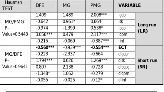
Table 5: Panel-ARDL estimation

VARIABLE PMG MG DFE Hausman TEST Long run ) LR ( lgdpr 2.008*** 1.489 1.409 MG/PMG P-Value=0.5443 lsk 0.664 0.961* -0.642 lpop 0.538* -1.399 -0.974 lopen 2.117*** 0.479 3.056*** linf -0.387*** -0.069 -0.215 Short run ) SR ( ECT -0.554*** -0.939*** -0.560*** MG/DFE P-Value=0.9641 dlgdpr -0.664 -2.337 -0.223 dlsk 1.269*** 0.626 1.794*** dlpopg -0.728 2.138 0.807 dlopen -0.279 1.062 -1.348* dlinf -0.12* -0.025 -0.055

Source : Stata11

The PMG long run elasticity estimate is larger than the MG estimate; the adjustment coefficient is also marginally higher in the former. The PMG estimator by pooling across countries provides efficient and consistent estimates (Blackburne III and Frank, 2007). If, however, slop homogeneity is rejected, the MG estimates will be inconsistent. The PMG estimates are consistent in either case. The Hausman test rejects the null hypothesis that the PMG estimator is efficient with a significance level of 5 percent.

 Error correction threshold: It is clear that the error correction (-0.554) was as expected, negative and significant, within 6%. Each year, 45.5% of the imbalances of foreign direct investment balance are adjusted in the long term

 Long run : The coefficient for real GDP growth is positive and statistically significant. This means that marketseeking FDI is located in countries where the real GDP growth potential is high since it guarantees profitability of the projects. The results are in line with Elbadawi and Mwega [30], Onyeiwu and Shrestha [18], Krugell [29] the coefficient size found 2.008, and indicates that one unit change in the GDP will bring 2.008 unit changes in the total FDI inflows.

The effect of physical capital on foreign direct investment is statistically insignificant in all estimates; In terms of trade openness, the

results showed that there is a significant and significant impact on foreign direct investment in the long run, especially in the PMG estimation. The increase in the opening rate of trade by 1% leads to an increase of 2.1% in foreign direct investment. The inflation rate was significant and had a negative effect on foreign direct investment in the PMG estimation. The population growth rate was insignificant in all estimates

most of the variables are insignificant, except for the physical capital stock which was significant and its effect on foreign direct investment

5. conclusion:

The objective of this study was to shed light on the determinants of foreign direct investiment (FDI) in North African countries during the period 1980-2010. In order to undertake it we performed an econometric model based in panel data analysis for 10 countries. we have relied on dynamic panel models because they give efficient and consistent estimates results, which are better than static panel models.

The study model was estimated in three different ways: the Mean Group(MG), the Poold Mean Group (PMG)and dynamic fixed effects (DFE). These methods were compared using the Hausman test, and the PMG method was to be suitable for standard study. The results of the application of this method indicate that in the long term, foreign direct investment depends on the per capita GDP, we were able to determine that both the size of the economy, as measured by GDP, in previous years, positively affected the inflows of FDI, being strongly.. The degree trade openness also proved to be an important determinant of FDI, being highly significant as well Inflation (INFLATION) appears as an indicator of macroeconomic stability, presenting a negative sign

6. References :

- Baltagi, Badi H.(2001), Econometric Analysis of Panel Data, 2nd edition. New York: John Wiley &Sons, LTD.

- Benjamin de Prost (2012), Les deux formes d'IDE et

l'investissement productif : l'impact du taux de change réel,Thèse

de doctorat en sciences économiques, Université Panthéon Assas. - Im, K. S., Pesaran, M. and Shin, Y. (2003), Testing for Unit Roots

in Heterogeneous Panels, Journal of Econometrics 115.

- Kang Yong Tan (2006), apooled mean group analysis on aid

- Marcelo Braga Nonnemberg, Mario Jorge Cardoso de Mendonça (2001), the determinants of foreign direct investment

in developing countries, Brazil.

- Miguel D. Ramirezt(2006), A Panel Unit Root and Panel

Cointegration Test ofthe Complementarity Hypothesis in theMexican Case(1960-2001), New Haven, CT 06520-8269.

- Murshed Chowdhury(2012),Panel Cointegration and Pooled

Mean Group Estimations of Energy Output Dynamics in South Asia, Journal of Economics and Behavioral StudiesVol. 4, No. 5, May

(ISSN: 2220-6140)

- Nunnenkamp, Peter & SPATZ, Julius(2002),Determinants of FDI

in developing countries: has globalization changed the rules of the game?, Transnacional Corporations, vol 11 (2).

- Pedroni, P. (1999), Critical Values for Cointegration Tests in

Heterogeneous Panels with Multiple Regressors, Oxford Bulletin

of Economics and Statistics 61.

- Pesaran, M.H., Shin, Y., Smith, R.P (1999), Pooled mean group

estimation of dynamic heterogeneous panels, Journal of the

American Statistical Association 94.

- S.Onyeiwu, H.Shrestha (2004), Determinants of Foreign Direct

Investment in Africa, Journal of Developing Societies, 89-106.

- Sutana Thanyakhan (2008), the determinants of FDI and FPI in

Thailand: a gravity model analysis, a Thesis submitted in partial

fulfillment of the requirements for the Degree of Doctor of Philosophy in Economics Lincoln University.

- W.Krugell, The Determinants of Foreign Direct Investment in

Africa, Multinational Enterprises, Foreign Direct Investment and

Growth in Africa M.Gilroy, T.Gries, W.A.Naudé (Eds.),

Physica-Verlag Heidelberg, New York, pp.49-71.