Adaptive Scheduling in Spark
by
Rohan Mahajan
Submitted to the Department of Electrical Engineering and Computer
Science
in partial fulfillment of the requirements for the degree of
Master of Engineering in Computer Science and Engineering
at the Massachusetts Institute of Technology
June 2016
c
○ Massachusetts Institute of Technology 2016. All rights reserved.
Author . . . .
Department of Electrical Engineering and Computer Science
May 20, 2016
Certified by . . . .
Prof. Matei Zaharia
Thesis Supervisor
Accepted by . . . .
Dr. Christopher J. Terman
Chairman, Masters of Engineering Thesis Committee
Adaptive Scheduling in Spark
by
Rohan Mahajan
Submitted to the Department of Electrical Engineering and Computer Science on May 20, 2016, in partial fulfillment of the
requirements for the degree of
Master of Engineering in Computer Science and Engineering
Abstract
Because most data processing systems are distributed in nature, data must be transferred between machines. Currently, Spark, a prominent such system, predetermines the strategies for shuffling this data, but in certain situations, different shuffle strategies would improve performance. We add functionality to track metrics about the data during the job and appro-priately adapt the shuffle strategy. We show improvements in ShuffledRDD performance, joins using Spark’s RDD interface, and joins in Spark SQL.
Acknowledgments
First, I would like to thank my parents Umesh Mahajan and Manjula Mahajan for their enduring support and love throughout my time at MIT.
I would like to thank Professor Matei Zaharia for his guidance, patience, and support while advising me throughout this project. I learned a lot throughout this project and am extremely grateful for the support.
At MIT, my work would never have been completed if not for the support of my friends. I would like to thank them for all the lessons that I have learned and all of the memories that I have created.
Contents
1 Introduction 13
1.1 Spark and MapReduce . . . 13
1.2 Shuffle . . . 13
1.2.1 Shuffle Introduction . . . 13
1.2.2 Shuffle Analysis . . . 15
1.3 Adaptive Scheduling of Joins . . . 15
1.3.1 Join Basics . . . 15
1.3.2 Shuffle Join . . . 16
1.3.3 Broadcast Join . . . 17
2 Implementation 21 2.1 Spark . . . 21
2.2 ShuffledRDD . . . 21
2.3 Joins . . . 22
2.3.1 ShuffleReader Changes . . . 22
2.3.2 ShuffledJoinRDD and BroadcastJoin RDD . . . 22
2.3.3 Joins in Spark SQL . . . 23
3 Experiments 25 3.1 Setup . . . 25
3.2 Regular Shuffle . . . 25
3.3 Broadcast and ShuffleJoinRDD . . . 26
4 Future Research and Conclusion 31
4.1 Future Research . . . 31
4.1.1 Extensions of Shuffle . . . 31
4.1.2 Extensions of Join . . . 31
4.2 Conclusion . . . 32
List of Figures
1-1 Shuffle for Letter Count in MapReduce . . . 14
1-2 Unbalanced Shuffle . . . 16
1-3 Balanced Shuffle . . . 17
1-4 Typical Shuffle Join . . . 18
1-5 Broadcast Join . . . 19
3-1 ShuffledRDD vs ShuffledRDD2 . . . 26
3-2 ShuffledRDD vs ShuffledRDD2 . . . 27
3-3 BroadcastJoinRDD vs ShuffleJoinRDD . . . 28
List of Tables
1.1 Table for Dataset 1 . . . 15 1.2 Table for Dataset 2 . . . 15 1.3 Table for Joined Data . . . 16
Chapter 1
Introduction
1.1
Spark and MapReduce
New data processing systems such as Spark and MapReduce have been designed to help process the increasing amount of data [2] [5]. Instead of relying on just one powerful computer, these systems use many computers due to lower costs, increased scalability, and improved fault tolerance. Because these systems are distributed in nature, they have stages (shuffle stages) where they transfer information between computers.
1.2
Shu
ffle
We will use MapReduce to explain the shuffle in more detail, but the main concepts still apply to Spark.
1.2.1
Shu
ffle Introduction
In the first stage of MapReduce, the map phase, the data is loaded onto different computers and computation is performed on this data that results in a group of key-value pairs. The final phase of MapReduce, the reduce phase, assumes that all key-value pairs with the same key are grouped together onto the same machine. We call this property the shuffle guarentee. Thus, the shuffle phase, an intermediate phase that the system handles internally,
transfers key-value pairs between machines to satisfy the shuffle guarentee.
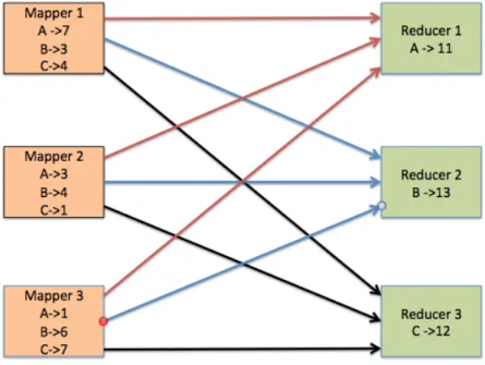
Figure 1-1 display the inner workings of the shuffle phase. For instance, a programmer may want to count the number of letters in a distributed file. The mappers will each load part of the distributed file and count the number of letters in their part. However, the systems needs to aggregate the count for each letter and thus all the counts for letter A will be sent to Reducer 1, letter B will be sent to Reducer 2, and letter C will be sent to Reducer 3. These reducers will then promptly aggregate the counts that they receive from the mappers.
Figure 1-1: Shuffle for Letter Count in MapReduce
This figures demonstrates a basic shuffle in MapReduce. Each mapper sends its letter counts to different reducers such that each reducer gets the total letter count for a specific letter.
Due to the huge amounts of keys, these systems do not transfer data on the granurality of keys. Instead, they use partitions, which contain key-value pairs with different keys. Programmers can pick different partitioning functions such as hash partitiong and range partitiong to map keys to partitions. Two identical keys are guarenteed to be in the same partition. As long as all the mappers partition their data in the same way and send each partition with the same index to the same reducer, the system satisfies the shuffle guarentee.
1.2.2
Shu
ffle Analysis
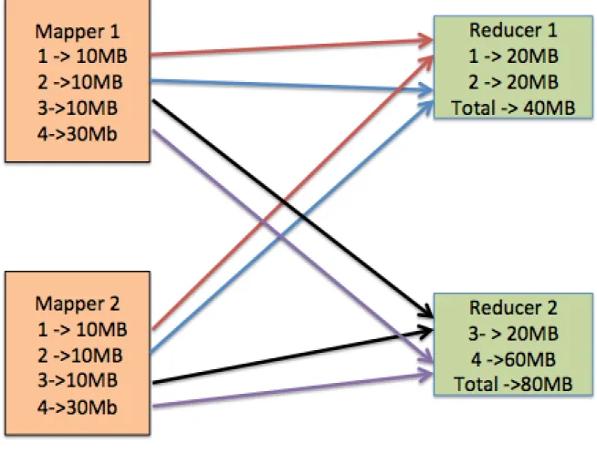
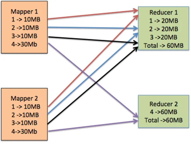
MapReduce is constrained by the slowest worker; therefore, minimizing the latency of the slowest worker should improve performance. Balancing the amount of data sent to each reducer helps achieve this by reducing both network latency and also the execution time for the slowest worker. Figure 1-2, depicts a shuffle scenario that results in unbalanced paritions. A basic heuristic is used with each reducer getting half of the mapper output partitions. Generally, this protocol should result in balanced reducers, but as seen, Reducer 2 receives twice the amount of data as Reducer 1. However, if the system knew the sizes of the map output partitions, it could more intelligently balance the reducers. As seen in Figure 1-3, with the same map output partitions, the system could attain complete balance of 60MB for each reducer.
1.3
Adaptive Scheduling of Joins
1.3.1
Join Basics
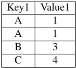
A common operation in these data processing environments is a join [3]. A join basically combines two tables by finding intersections between keys in respective columns. For in-stance, if we have Table 1.1 and Table 1.2 that we are trying to join based on the intersection of Key1 and Key2, the resulting output is Table 1.3
Key1 Value1
A 1
A 1
B 3
C 4
Table 1.1: Table for Dataset 1
Key2 Value2
A 5
C 7
Figure 1-2: Unbalanced Shuffle
Reducer 1 requests partitions 1 and 2 while Reducer 2 requests partitions 3 and 4. This results in Reducer 2 receiving 80MB of data while Reducer 1 receives only 40MB of data.
Key1 Value1 Value2
A 1 5
A 2 5
C 4 7
Table 1.3: Table for Joined Data
1.3.2
Shu
ffle Join
The actual implementation of joins in MapReduce is very similar to the shuffle scenario presented above. Instead of having output partitions for just one dataset, the mappers have output partitions for two datasets and ensure that all partitions for both datasets with the same index are sent to the same reducer. Figure 1-4 details a shuffle join. For both datasets, all of the keys that mapped to partition 1 were sent to Reducer 1 and this happens
Figure 1-3: Balanced Shuffle
Reducer 1 requests partition 1,2, and 3 while Reducer 2 requests partition 4. This results in both Reducer 1 and Reducer 2 receiving 60MB of data.
tively for the rest of the partitions. Because all identical keys are in the same partition and each partition with the same index is sent to the same reducer, the system is guarenteed to find all intersections required for the join.
1.3.3
Broadcast Join
The diagram above may seem to imply that mappers and reducers are different machines. However, this distinction is artificial and there are no seperate machines for mappers and reducers. Therefore, not all data in the shuffle stage is transferred over the network. In Figure 1-1, if Mapper 1 and Reducer 1 were the same machine, the key-value pair A=7 would be read locally and not have to be received over the network.
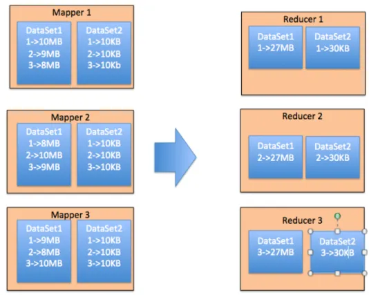
Figure 1-4: Typical Shuffle Join
This figure depicts a typical shuffle join. The mappers have output partitions for two dif-ferent datasets. They ensure that all the partitions with the same index get sent to the same reducer. Reducer 1 received partition 1, Reducer 2 received partition 2, and Reducer 3 received partition 3.
Because transferring data over the network could be a bottleneck [4], the broadcast join tries to increase the amount of data being read locally. For instance, in Figure 1-4, Dataset 1 is drastically bigger than Dataset 2. As seen in Figure 1-5, the broadcast join keeps the bigger dataset in place and sends the entirety of Dataset 2 to every reducer. Even though all of Dataset 1 stays in place, this method will still find all intersections beteen the datasets because all partitions of Dataset 2 are sent to every reducer. The diagram shows that only Dataset 2 is transferred and thus the network traffic is reduced from megabytes to kilobytes. Broadcast Join is not always the optimal strategy. Because the entirety of the smaller dataset is sent to every partition, the amount of total computation time increases. Addition-ally, if the datasets are approximately the same size, network traffic will actually increase. Each join strategy is the optimal strategy in different situations. Thus, it becomes impera-tive to pick the strategy after the mappers have run and the size of the map output partitions
is known.
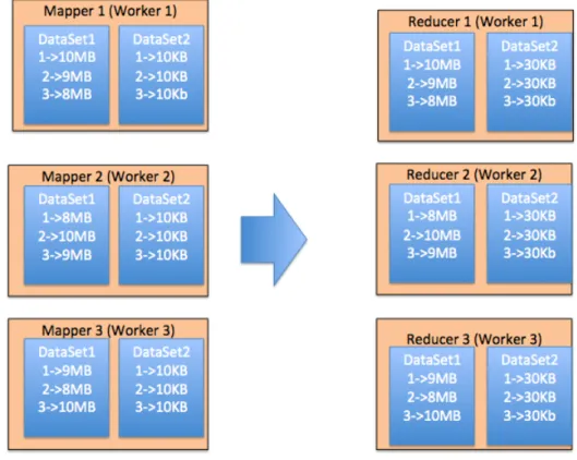
Figure 1-5: Broadcast Join
This figure depicts a Broadcast Join. As evidenced, the bigger dataset stays entirely in place but the entirety of the smaller dataset is sent to the each reducer. This cuts network traffic from megabytes to kilobytes.
Chapter 2
Implementation
2.1
Spark
All of the code was implemented in Spark but could also be implemented in MapReduce to achieve similar performance improvements. The Resilient Distributed Dataset(RDD) is the main programming interface within Spark. An RDD can be created from data or from another RDD. The key attributes of an RDD are its inputs, the number of partitions, and how each of its partitions is computed based on its inputs.
Profressor Matei Zaharia added code that allowed the tracking of sizes of map output partitions.
2.2
Shu
ffledRDD
The RDD we developed is a new version of ShuffledRDD, ShuffledRDD2. Its inputs are first a shuffle dependency, which is basically a bunch of map output partitions, and second, a number of reducers, or equivalentally the number of partitions for ShuffledRDD2. In the regular ShuffledRDD, each of its partition naively requests a segment of map output parti-tions as depicted in Figure 1-2. ShuffledRDD2 implements the more complicated scheme seen in Figure 1-3. The current Spark API only allows reducer partitions to request consec-utive map partitions. In other words, it is impossible for a ShuffledRDD2 partition to have map output partitions 1 and 3, without having 2. For this constraint and the given number
of reducer partitions, ShuffleRDD2 assigns map output partitions to optimally balance the number of bytes received by each of its reduce partitions.
2.3
Joins
2.3.1
Shu
ffleReader Changes
In the broadcast join, the bigger RDD must stay in place. The current interface only allows a reducer to request a specific map output partition from all of the mappers. For the bigger RDD, the system would then have to request map output partitions from other machines, which defeats the purpose of the broadcast join. Thus, we added the capability of requesting a specific partition from just one mapper.
2.3.2
Shu
ffledJoinRDD and BroadcastJoin RDD
We implement two different type of RDDs, the ShuffledJoinRDD and the BroadcastJoin-RDD. Both of these RDD’s take two shuffle dependencies, which remember are basically the outputs of map stages, partitioned in a certain way. These dependencies must be parti-tioned in the same way; otherwise, two identical keys would not map to the same partition index.
The ShuffledJoinRDD implementation is very similar to ShuffledRDD. Instead of fetch-ing map output partitions from just one dependency, it fetches the correspondfetch-ing map out-put partitions from both dependencies. The user specificies the number of Shu ffledJoin-RDD partitions and each paritition requests a corresponding fraction of the map output partitions. For instance, ShuffledJoinRDD partition 1 will fetch Dataset1 Partition 1 and Dataset2 Partition 1 from all of the workers. Once these partitions are fetched, it creates a map with the key-value pairs of the smaller partition. Subsequently, it iterates through the keys of the bigger partition, seeing if they are present in this map, and if so, adding the intersection to the output.
The BroadcastJoinRDD implements the broadcast shuffle. Each BroadcastJoinRDD partition requests one local map output partition from the bigger RDD using the new request
capability and all of the paritions from the smaller RDD. The number of partitions is equal to the number of partitions of the bigger input RDD. We use the location preferences api of the RDD to ensure that the reducer partitions are placed on the same machines that the mapper partition it is requesting was originally on, to ensure data is requested locally instead of over the network. The system use the same strategy with the map and the iteration as the ShuffledJoinRDD to then find the intersections.
2.3.3
Joins in Spark SQL
Many programmers and data analysts prefer not to use the RDD interface and are more familiar with SQL; thus, Spark offers a SQL like interface or SparkSQL [1]. One popular operation within SQL is join [2]. Although the user still writes in SQL, Spark still executes the code using RDDs.
Because we are not just using the RDD interface and Spark automatically converts the SQL query into a query plan, the implementation is much more complicated and thus we only implement our optimization for sort-merge join. Although the exact semantics for how a sort-merge join can be found here[6], the sort-merge join still must shuffle data around as it requires that every key that could intersect should be sent to the same reducer. To help achieve this, the sort-merge join applies an exchange operator on each of the map outputs. These exchange operators produce ShuffleRowRDDS, which for our purposes are equivalent to ShuffledRDDs. In the next stage, each partition in the first ShuffledRowRDD is compared to the partition with the same index in the second ShuffledRowRDD. The only difference between this and how the join RDDs work is pretty semantic in that instead of one RDD requesting partitions from multiple mappers, two RDD’s repartition their data and then another one compares them partition by partition. By default, the code performs a shuffle join almost exactly in a manner with how the ShuffledJoinRDD works. One ShuffleRowRDD requests the corresponding partitions from its mappers just like Figure 1-2 and the other ShuffleRowRDD does the exact same but with its dataset.
However, if only one input RDD is smaller then a user-configured threshold, the sys-tem uses the broadcast join optimization. The bigger ShuffledRowRDD will be exactly
like its parent. We achieve this by setting number of partitions for the ShuffledRowRDD to be equal to its parent and then having each partition request a specific partition from the parent using the new request api and set its location preference accordingly. The other ShuffledRowRDD will have the same number of partitions as the bigger ShuffledRowRDD with each partition containing the entirety of the smaller input RDD. The correctness guar-entees are the same as the BroadcastJoinRDDs.
Chapter 3
Experiments
3.1
Setup
All jobs were run using the Spark interactive shell. All jobs were run ten times, with the last five times being averaged. All local jobs were run on a 2013 MacbookPro with 8GB of RAM and 2 cores. All distributed jobs were run using the spark-ec2 launch scripts. They were run on four AWS m1.large machines in the us west zone.
3.2
Regular Shu
ffle
We compared the performance of ShuffledRDD vs ShuffledRDD2 both on a local machine and on a distributed cluster.
For the local machine test, we created four mapper partitions. One mapper partition was three times the size of the other mapper partitions. We created two reducer partitions. For the the regular ShuffledRDD, each reducer got two mapper patitions, which results in one reducer partition having twice the amount of data. For the ShuffledRDD2, one reducer requests the three smaller map partitions while the other received just the bigger partition, resulting in balanced partitions. As seen in Figure 3-1, the ShuffledRDD2 performs better as it has more balanced reducers.
For the distributed test, we created 64 mapper partitions. One mapper patition was significantly bigger and equal to 8 regular mapper partitions. We had 8 reducers. In the
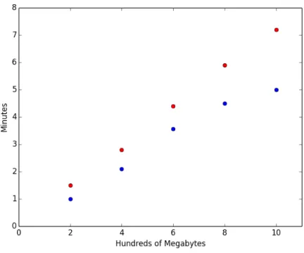
Figure 3-1: ShuffledRDD vs ShuffledRDD2
This figure measures the local machine performance of joins completed using the Shu ffle-dRDD versus the ShuffledRDD2. The ShuffledRDD is in red while the ShuffledRDD2 is in blue. In the ShuffledRDD, Reducer 1 gets twice the amount of data as Reducer 2, but in the ShuffledRDD2, Reducer 2 receives the same amount of data. The x axis indicates how much data was shuffled.
ShuffledRDD, one of these reducers approximately had twice the amount of data as the others, but in the ShuffledRDD2 they were all balanced. Figure 3-2 shows that just like in the local tests, ShuffledRDD2 performs better in the distributed tests.
3.3
Broadcast and Shu
ffleJoinRDD
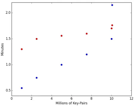
For this test, we created a bigger RDD with key-value pairs of (x, 2 * x) with x ranging from 1 to 100 milllion. As seen in the Figure 3-3, we then then manipulated the number of key-value pairs of the smaller RDD, with each key value pairs being (x,x). We measured the performance for the ShuffleJoinRDD and BroadcastJoinRDD on a the distributed cluster. As expected, initially the BroadcastJoinRDD performs better as it requires significantly less network traffic. However, it soon becomes slower than the ShuffleJoinRDD as the
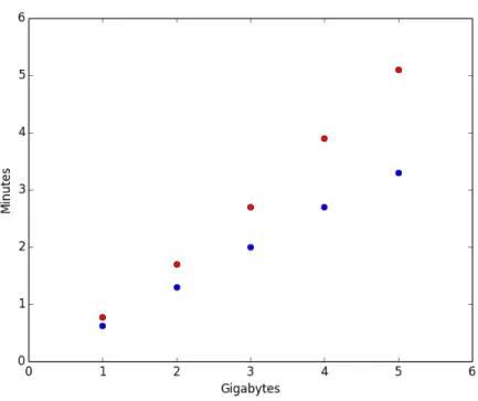
Figure 3-2: ShuffledRDD vs ShuffledRDD2
This figure measures the performance of joins completed using the ShuffledRDD versus the ShuffledRDD2. The ShuffledRDD is in red while the ShuffledRDD2 is in blue. We had eight reducers. In the ShuffledRDD, one reducer gets twice the amount of data as the other reducers, but in the ShuffledRDD2 they all receive the same amount of data. The x axis indicates how much data was shuffled.
smaller input RDD increases. Increasing the smaller RDD does not dramatically influence the ShuffleJoinRDD as it is more bottlenecked by the bigger RDD and just sends pieces of the smaller RDD to each partition. However, this increase significantly influences the BroadcastJoinRDD because it transmits the entirety of the smaller RDD to every partition.
3.4
Spark SQL Join
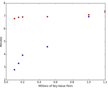
We evaluated the performance of the sort-merge join using the broadcast strategy and the shuffle strategy in Spark SQL on a distributed cluster. For this test, we created a bigger RDD with key-value pairs of (x, 2 * x) with x ranging from 1 to billlion. As seen in the Figure 3-4, we then then manipulated the number of key-value pairs of the smaller RDD, with each key value pairs being (x,x). We then converted these into dataframes, the main
Figure 3-3: BroadcastJoinRDD vs ShuffleJoinRDD
This figure measures the performance of joins completed using the BroadcastJoinRDD versus the ShuffleJoinRDD. The BroadcastJoinRDD is in blue while the ShuffleJoinRDD is in red. The bigger RDD is fixed with 100 million key-value pairs, but the number of key-value pairs of the small RDD is manipulated along the x axis.
interface for Spark SQL, and then used Spark SQL to join them. We used 30 partitions for both the shufle and the broadcast tests and turned off map output compression. Initially, the broadcast performs better as it requires significantly less network traffic. However, it soon becomes slower then the shuffle as the smaller input RDD increases just like what happened with the join RDDs. Increasing the smaller input dataset is way worse in the broadcast than the shuffle because the broadcast sends its entirety to each partition while the shuffle does not. Thus, if the input dataset is sufficiently small, the shuffle performs better, but otherwise the broadcast performs better.
Figure 3-4: Broadcast vs Shuffle in Spark SQL
This figure measures the performance of sort-merge join in Spark SQL. The broadcast strategy is in blue while the shuffle join is in red. The bigger RDD is fixed with 1 billion key-value pairs, but the number of key-value pairs of the small RDD is manipulated along the x axis.
Chapter 4
Future Research and Conclusion
4.1
Future Research
4.1.1
Extensions of Shu
ffle
ShuffledRDD2 is limited in a couple ways. First, each reducer can fetch multiple partitions, but these partitions are internally fetched individually. Batching these partition requests together could help reduce overhead. Second, the current version only supports inputing the number of reducers. Users could prefer an interface where they input the maximum number of bytes a reducer can have and then the system automatically determines the number of reducers.
4.1.2
Extensions of Join
First, we implement our changes in the exchange framework to make the easiest possible change to allow for our optmization, but we could conceivably do this in a cleaner manner. Second, users have to statically pass in thresholds that determine when to switch be-tween broadcast and shuffle joins. The system should automatically determine this based on factors such as the size of the input RDDs, the network bandwith, and the memory of each machine.
Third, we either broadcast an entire RDD or default to the shuffle pattern. However, if RDD1 has a big partition 1 and a small partition 2 and RDD2 has a small partition 1 and
big partition 2, the systems performs a shuffle. However, the system could save time by having RDD1 broadcast its partition 1 and RDD2 broadcast its partition 2.
Fourth, in the broadcast join in Spark SQL, each reducer partition requests the entirety of its input. This request is made over the network for each partition, but generally multiple reducer partitions are on the same machine. Thus, a request should be made once per machine and stored in memory for the other partitions to use.
4.2
Conclusion
In conclusion, we show that improvements can be made to the shuffle stage of Spark. In-stead of predetermining our shuffle strategy, we can adapt it based on the output of the mappers. We show that these stategies improve the regular shuffle RDD, joins with RDDs, and joins in Spark SQL. Although we have shown improvements, the work can be extended with simple changes to further improve performance.
Bibliography
[1] Michael Armbrust, Reynold S. Xin, Cheng Lian, Yin Huai, Davies Liu, Joseph K. Bradley, Xiangrui Meng, Tomer Kaftan, Michael J. Franklin, Ali Ghodsi, and Matei Zaharia. Spark sql: Relational data processing in spark. In Proceedings of the 2015 ACM SIGMOD International Conference on Management of Data, SIGMOD ’15, pages 1383–1394, New York, NY, USA, 2015. ACM.
[2] Jeffrey Dean and Sanjay Ghemawat. Mapreduce: Simplified data processing on large clusters. Commun. ACM, 51(1):107–113, January 2008.
[3] Priti Mishra and Margaret H Eich. Join processing in relational databases. ACM Com-puting Surveys (CSUR), 24(1):63–113, 1992.
[4] Kay Ousterhout, Ryan Rasti, Sylvia Ratnasamy, Scott Shenker, and Byung-Gon Chun. Making sense of performance in data analytics frameworks. In 12th USENIX Sympo-sium on Networked Systems Design and Implementation (NSDI 15), pages 293–307, Oakland, CA, 2015. USENIX Association.
[5] Matei Zaharia, Mosharaf Chowdhury, Tathagata Das, Ankur Dave, Justin Ma, Murphy McCauley, Michael J. Franklin, Scott Shenker, and Ion Stoica. Resilient distributed datasets: A fault-tolerant abstraction for in-memory cluster computing. In Proceedings of the 9th USENIX Conference on Networked Systems Design and Implementation, NSDI’12, pages 2–2, Berkeley, CA, USA, 2012. USENIX Association.
[6] Jingren Zhou. Sort-merge join. In Encyclopedia of Database Systems, pages 2673– 2674. Springer, 2009.