HAL Id: hal-03047833
https://hal.archives-ouvertes.fr/hal-03047833
Submitted on 9 Dec 2020
HAL is a multi-disciplinary open access
archive for the deposit and dissemination of
sci-entific research documents, whether they are
pub-lished or not. The documents may come from
teaching and research institutions in France or
abroad, or from public or private research centers.
L’archive ouverte pluridisciplinaire HAL, est
destinée au dépôt et à la diffusion de documents
scientifiques de niveau recherche, publiés ou non,
émanant des établissements d’enseignement et de
recherche français ou étrangers, des laboratoires
publics ou privés.
ice-shelf collapse (ABUMIP)
Sainan Sun, Frank Pattyn, Erika Simon, Torsten Albrecht, Stephen Cornford,
Reinhard Calov, Christophe Dumas, Fabien Gillet-Chaulet, Heiko Goelzer,
Nicholas Golledge, et al.
To cite this version:
Sainan Sun, Frank Pattyn, Erika Simon, Torsten Albrecht, Stephen Cornford, et al.. Antarctic ice
sheet response to sudden and sustained ice-shelf collapse (ABUMIP). Journal of Glaciology,
Interna-tional Glaciological Society, 2020, 66 (260), pp.891-904. �10.1017/jog.2020.67�. �hal-03047833�
Article
Cite this article:Sun S et al. (2020). Antarctic ice sheet response to sudden and sustained ice-shelf collapse (ABUMIP). Journal of Glaciology 66(260), 891–904. https://doi.org/ 10.1017/jog.2020.67
Received: 31 December 2019 Revised: 17 July 2020 Accepted: 20 July 2020
First published online: 14 September 2020 Keywords:
Antarctic glaciology; ice-sheet modelling; ice shelves
Author for correspondence: Sainan Sun,
E-mail:[email protected]
© The Author(s) 2020. This is an Open Access article, distributed under the terms of the Creative Commons Attribution licence (http:// creativecommons.org/licenses/by/4.0/), which permits unrestricted re-use, distribution, and reproduction in any medium, provided the original work is properly cited.
cambridge.org/jog
sustained ice-shelf collapse (ABUMIP)
Sainan Sun1, Frank Pattyn1 , Erika G. Simon2, Torsten Albrecht3 ,
Stephen Cornford4, Reinhard Calov3, Christophe Dumas5,
Fabien Gillet-Chaulet6 , Heiko Goelzer1,7, Nicholas R. Golledge8,
Ralf Greve9,10 , Matthew J. Hoffman11 , Angelika Humbert12,13,
Elise Kazmierczak1, Thomas Kleiner12 , Gunter R. Leguy14,
William H. Lipscomb14, Daniel Martin15 , Mathieu Morlighem16 ,
Sophie Nowicki2, David Pollard17, Stephen Price11, Aurélien Quiquet5,
Hélène Seroussi18 , Tanja Schlemm3,19, Johannes Sutter12,20,
Roderik S. W. van de Wal7, Ricarda Winkelmann3,19 and Tong Zhang11
1
Laboratoire de Glaciologie, Université libre de Bruxelles (ULB), Brussels, Belgium;2NASA/GSFC, Greenbelt MD, USA;3Potsdam Institute for Climate Impact Research (PIK), Member of the Leibniz Association, P.O. Box 601203, 14412, Potsdam, Germany;4Department of Geography, Swansea University, Swansea, UK;5Laboratoire des Sciences du Climat et de l’Environnement, LSCE/IPSL, CEA-CNRS-UVSQ, Université Paris-Saclay, F-91191 Gif-sur-Yvette, France;6Univ. Grenoble Alpes/CNRS/IRD/G-INP, Institut des Géosciences de l’Environnement, 38000 Grenoble, France;7Institute for Marine and Atmospheric Research, Utrecht University, The Netherlands;8Antarctic Research Centre, Victoria University of Wellington, New Zealand;9Institute of Low Temperature Science, Hokkaido University, Sapporo, Japan;10Arctic Research Center, Hokkaido University, Sapporo, Japan;11Theoretical Division, Los Alamos National Laboratory, Los Alamos NM, USA;12Alfred-Wegener-Institut, Helmholz-Zentrum für Polar und Meeresforschung, Bremerhaven, Germany;13Department of Geoscience, University of Bremen, Bremen, Germany;
14
Climate and Global Dynamics Laboratory, National Center for Atmospheric Research, Boulder CO, USA;
15
Lawrence Berkeley National Laboratory, Berkeley CA, USA;16Department of Earth System Science, University of California Irvine, Irvine, USA;17Pennsylvania State University, EMS Earth and Environmental Systems Institute, Pennsylvania, USA;18Jet Propulsion Laboratory, California Institute of Technology, Pasadena, USA;19University of Potsdam, Institute of Physics and Astronomy, Karl-Liebknecht-Str. 24-25, 14476, Potsdam, Germany and20Climate and Environmental Physics, Physics Institute and Oeschger Centre for Climate Change Research, University of Bern, Bern, Switzerland
Abstract
Antarctica’s ice shelves modulate the grounded ice flow, and weakening of ice shelves due to climate forcing will decrease their ‘buttressing’ effect, causing a response in the grounded ice. While the processes governing ice-shelf weakening are complex, uncertainties in the response of the grounded ice sheet are also difficult to assess. The Antarctic BUttressing Model Intercomparison Project (ABUMIP) compares ice-sheet model responses to decrease in buttres-sing by investigating the ‘end-member’ scenario of total and sustained loss of ice shelves. Although unrealistic, this scenario enables gauging the sensitivity of an ensemble of 15 sheet models to a total loss of buttressing, hence exhibiting the full potential of marine ice-sheet instability. All models predict that this scenario leads to multi-metre (1–12 m) sea-level rise over 500 years from present day. West Antarctic ice sheet collapse alone leads to a 1.91–5.08 m sea-level rise due to the marine ice-sheet instability. Mass loss rates are a strong func-tion of the sliding/fricfunc-tion law, with plastic laws cause a further destabilizafunc-tion of the Aurora and Wilkes Subglacial Basins, East Antarctica. Improvements to marine ice-sheet models have greatly reduced variability between modelled ice-sheet responses to extreme ice-shelf loss, e.g. compared to the SeaRISE assessments.
Introduction
The vast majority of Earth’s freshwater is stored in the Antarctic ice sheet and because of this large volume (>55 m sea-level equivalent (SLE); Nowicki and others, 2013; Albrecht and others, 2020; Morlighem and others, 2020), the loss of even a small fraction of its mass could soon dominate sea-level rise. Reconstructions of past sea level show that the ice sheet could have contributed between 10 and 20 m SLE during the Pliocene, a period stretching between 5.3 and 2.6 million years before present with global mean temperature 2--3◦C higher than present-day (Miller and others,2012; Grant and others,2019). Current observed mass loss from the Antarctic ice sheet is accelerating and concentrated in the Amundsen Sea area (Mouginot and others,2014; Rignot and others,2014; Shepherd and others,2018) and the Aurora Subglacial Basin, including Totten Glacier (Khazendar and others, 2013). These changes have been attributed to variations in ocean circulation bringing warm, intermediate-depth waters into contact with the base of ice shelves (Payne and others,2004; Thomas and others,2004; Jenkins and others,2010; Pritchard and others, 2012; Paolo and others,2015; Jenkins and others,2018).
Despite recent advances in modelling marine ice sheets (Pattyn, 2018), projections of the future contribution of the Antarctic ice sheet to sea level are still hampered by insufficient knowledge of atmospheric and oceanic forcings and the impact of those forcings on critical ice-sheet model physics and dynamics (Pattyn and others,2018). This is exemplified by the hypothesis of new physical mechanisms, such as the Marine Ice Cliff Instability (MICI; Bassis and Walker,2012; Pollard and others,2015), which leads to significantly larger sea-level contributions for the Antarctic ice sheet compared to other studies (DeConto and Pollard,2016). However, additional studies conclude that major ice loss during the Pliocene Epoch could also be reached without such mechanisms (Bulthuis and others, 2019; Edwards and others, 2019; Golledge and others, 2019). Other uncertainties stem from the timing and processes that govern ice-shelf weaken-ing, disintegration and collapse (Pattyn and others,2018).
Thinning of ice shelves, and concomitant reduction in ice-shelf buttressing, leads to grounding line retreat, inland ice accel-eration and loss of grounded ice mass (Pritchard and others, 2012). Reduction in ice-shelf buttressing has an almost instantan-eous effect on ice flow, which implies that this process can result in rapid changes in ice flux over the grounding line (Reese and others, 2018b; Gudmundsson and others, 2019). Ice-shelf thin-ning and weakethin-ning due to specific interactions with atmosphere (surface melt, meltwater percolation, refreezing and runoff; Trusel and others,2015) and ocean (changes in ocean circulation, ocean warming and sub-ice-shelf melting; Alley and others, 2015; Thompson and others,2018) are parameterized with a large vari-ation in ice-sheet models (Favier and others,2019).
In this paper, we investigate how changing ice shelves control Antarctic mass loss independent of the triggers for how and when ice shelves weaken. Previous ice-sheet intercomparison efforts (Pattyn and others, 2012, 2013; Bindschadler and others, 2013; Nowicki and others,2013; Seroussi and others,2019) highlighted the importance of better assessing the causes of the variation in model results, and separating differences associated with model grid resolution, ice dynamics (e.g. choice of stress balance equa-tion), physical processes included (e.g. calving, hydrofracture and cliff failure), initialization procedure (e.g. data assimilation, spin-up or relaxation) and numerical schemes. We designed a simple experiment that considers an instantaneous and sustained removal of floating ice. This scenario is not realistic, but allows us to investigate how different ice-sheet models cope with the impact of a sudden, complete loss of ice-shelf buttressing. By removing the uncertain causes related to ice-shelf thinning and weakening, we are able to isolate uncertainties in the response of the grounded ice sheet to grounding-line retreat due to loss of ice-shelf buttressing. We analyse 15 simulations from 13 international groups in order to determine the most relevant factors controlling the rate of Antarctic mass changes in an extreme mass loss scen-ario. Furthermore, the absence of buttressing may lead to ice-sheet collapse through the marine ice-ice-sheet instability (MISI) in areas where the bed deepens towards the interior of the ice sheet. The experiment therefore enables to quantify the MISI potential and associated uncertainties for the Antarctic ice sheet and revises estimates of this potential that have previously been made for the West Antarctic ice sheet (Bamber and others,2009). This experiment is coordinated through the Antarctic BUttressing Model Intercomparison Project, ABUMIP ( http://www.climate-cryosphere.org/wiki/index.php?title=ABUMIP-Antarctica), endorsed by the Ice Sheet Model Intercomparison Project, ISMIP6 (http://www.climate-cryosphere.org/activities/ targeted/ismip6), part of the Coupled Model Intercomparison project, CMIP6 (https://www.wcrp-climate.org/wgcm-cmip/ wgcm-cmip6). It builds on the ISMIP6 initialization experiments (
http://www.climate-cryosphere.org/wiki/index.php?title=InitMIP-Antarctica) for the Antarctic ice sheet (Seroussi and others,2019), in which most of the models in this study participated (see Appendix for details on each model). The main purpose of ABUMIP is to gauge the sensitivity of different ice-sheet models with respect to such grounding-line retreat, whether they pertain to numerical methods, physical approximations or boundary con-ditions. It also enables evaluation of the sensitivity of models that are used for the full Antarctic, for global sea-level rise projections (Seroussi and others,2019). While similar experiments have been done previously by Cornford and others (2016), Golledge and others (2017, supplementary material) and Pattyn (2017), we are able to put these results into a wider context through a controlled experiment and by examining a large number of diverse models. This will help to better understand the spread in projections of 21st century Antarctic ice sheet contributions to sea level.
Experiments and model setup Description of the experiments
ABUMIP consisted of three experiments, a control run (ABUC) and two forcing experiments (ABUK and ABUM) that controlled the rate of loss of ice shelves. All experiments started from an initi-alized present-day state of the Antarctic ice sheet, as defined by the initMIP-Antarctica (Seroussi and others, 2019). All ABUMIP experiments ran for a period of 500 years forward in time.
Control run (ABUC)
Similar to Seroussi and others (2019), atmospheric and oceanic forcings in the control run were assumed to be similar to present-day conditions, without any extra forcing aside from that applied at the end of the initialization.
Ice-shelf removal or‘float-kill’ (ABUK)
For the first forcing experiment, all floating ice (ice shelves) surrounding the ice sheet was removed at the start of the run and thereafter any newly-formed floating ice was instantaneously removed (so-called‘float-kill’). In other words, at all times, calv-ing flux was assumed to be larger than the flux across the ground-ing line to prohibit regrowth of the shelves.
Extreme sub-ice-shelf melt (ABUM)
The second experiment applied an extremely high constant melt rate of 400 m a−1underneath the ice shelves. Similar experiments have been carried out in previous studies with basal melt rates ranging from 200 m a−1 in Bindschadler and others (2013) to 400 m a−1 in Cornford and others (2016). Such high forcings inevitably lead to rapid loss of ice shelves and hence of buttres-sing. Preliminary experiments have shown that the actual value within the range found in the literature is of lesser importance.
Model setup
Participating ice-sheet models were free to choose the initializa-tion procedure, which is generally dependent on the given model characteristics and requirements. There were no further constraints on present-day forcing datasets applied (including surface mass balance, surface temperature and sub-shelf melt rates) or on specific physical processes and parameterizations included in the models (e.g. basal sliding and friction laws, ice rheology and stress balance approximation). Isostatic adjustment was not considered. The initialization time varies among models but was near the beginning of the 21st century.
Models were required to represent ice shelves and grounding line dynamics, and the initialization process should include ice shelves. Ice-sheet models applied the present-day surface mass balance
(SMB) and basal mass balance (BMB) of their choice, but without adjusting for the impacts of geometric changes in the forward experi-ments (i.e. no SMB, surface-elevation feedback). Finally, models used the bed and surface topography of their choice, while bedrock eleva-tion adjustment and processes affecting ice shelves (other than sub-shelf melting) were not taken into account. Model output was taken in the same format as for the initMIP-Antarctica experiments (Seroussi and others,2019) but for 500 years instead of 100 years after being initialized to the beginning of the 21st century.
Participating models
A total of 13 modelling groups participated in the experiments and most of these performed all the three experiments (Table 1). Details of the 15 different models, their initialization, their numerical characteristics and which sliding or friction laws are employed are summarized inTable 2. Time steps from 0.4 days to 0.5 years are used by models. Further description of the models can be found in the Appendix.
All models include membrane stresses in their force balance, either corresponding to the so-called Shallow-Shelf Approximation (SSA,Table 2), or by also including vertical shear-ing and vertically differentiated membrane stresses. The majority of models are hybrid models and heuristically combine the SSA as a sliding or friction law with the Shallow-Ice Approximation (SIA) for inclusion of vertical shearing (Bueler and Brown, 2009). One model includes vertical shear terms in the effective viscosity term (Schoof and Hindmarsh, 2010), which leads to the so-called SSA* approach. One model applies the Blatter– Pattyn approximation (labelled LMLa), which is the hydrostatic approximation of the Stokes equations (Blatter, 1995; Pattyn, 2003), and one model (labelled L1L2) uses a depth-integrated version of this approximation (Goldberg,2011).
The participating models use several different initialization techniques. A common approach is the paleo spin-up (Sp, Table 2) during which the ice sheet is run through a glacial-interglacial cycle until the present day. In this way, the state includes temperature field and change rates of geometry as cumu-lative response to past climates. In one case, the spin-up runs with an iterative optimization for basal friction coefficients with target values for ice thickness (SpC). Another common procedure is an equilibrium type spin-up, which also allows for establishing an internal temperature field with equilibrium ice sheet (Eq). In most cases, this equilibrium ice sheet is combined with an itera-tive optimization of the basal sliding/friction field to obtain an ice-sheet geometry that is close to the observed ice sheet (EqC), with methods described in Pollard and DeConto (2012b) and Le clec’h and others (2019), among others. All other models used data assimilation (essentially using the observed surface vel-ocity field) to tune a basal friction field in present day conditions (DA). While models employing paleo spin-up (Sp) or an equilib-rium state (Eq) have a present-day ice-sheet geometry that is in poorer agreement with the observed ice sheet (compared to mod-els using assimilation methods), assimilation-based initial condi-tions generally have noisier and more unrealistic ice thickness transients.
Apart from the wide range of initialization techniques, dis-cussed in more detail in Goelzer and others (2018) and Seroussi and others (2019), major model differences stem primarily from the basal sliding and/or friction law employed. Two commonly used basal conditions are the Weertman sliding (Weertman, 1957) and the Coulomb friction law (Schoof, 2005) (Table 2). Both can be written in the following generic form
tb=b2ub, (1)
whereτbis the basal shear stress (sum of all basal resistance), ubis
the basal sliding velocity, andβ2a friction term that in the case of a Weertman sliding law is defined by
b2= Cu1/m−1
b Np/m, (2)
where C is a friction coefficient that can be spatially varying for models that use a SpC, EqC or DA initialization techniques, and N represents the effective pressure at the base of the ice sheet (difference between the ice overburden pressure and subgla-cial water pressure). For m = 1, the friction law becomes viscous and β2 is solely dependent on the effective pressure. However, most models set p = 0 so that N is not considered, except ILTS-PIK-SICOPOLIS that uses p = 2. In the case of a Coulomb friction law the friction term is written using the expression as in Schoof (2005) or as in Aschwanden and others (2019)
b2= N tanf
ub
| |(1−q)uq 0
, (3)
whereϕ is the till friction angle that is either considered constant or optimized in a similar fashion to the friction term C in Eqn (2). The yield stressτcis defined by the numerator in Eqn (3), 0≤ q ≤ 1,
and u0represents a threshold speed for sliding (Aschwanden and
others, 2013). The friction law, Eqn (3), includes the case q = 0, leading to the purely plastic (Coulomb) relation τb=τcub/|ub|. In
the linear case q = 1, Eqn (3) becomesβ2=τc/u0(Bueler and van
Pelt,2015). Most models define the effective pressure N from till dynamics (Bueler and van Pelt, 2015; Aschwanden and others, 2019), which leads to a sharp contrast in effective pressure between saturated till and non-saturated till or hard bedrock. None of the models considered full subglacial hydrology but either define effect-ive pressure from subglacial elevation (submarine basins with satu-rated till) or from locally genesatu-rated subglacial melt. The last column ofTable 2lists the values of m and q for the different friction laws employed. One model uses a Weertman law limited by a Coulomb friction law (Table 2), in which the basal shear stress is set to the minimum of the two stresses (Tsai and others,2015).
Results ABUC
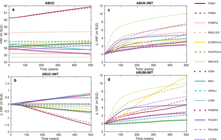
The standard experiment of the series is the control run (ABUC), where participating models run forward for 500 years starting from the initial conditions without any external forcing. This experiment allows for determining intrinsic model drift. Despite the lack of forcing, there is a large variation in ice-sheet mass changes observed (Fig. 1; expressed in terms of contribution to sea level based on the volume above flotation as defined in Eqn (1) of Bindschadler and others, 2013), depending on the initial dataset used. The method converting ice-sheet mass loss to sea-level contribution results in ∼56.7 m SLE based on the Bedmap2 data set, which is lower than the value 58.3 m in Fretwell and others (2013) using the Lambert Azimuthal Equal Area projection for area and volume calculations. For BedMachine Antarctica (Morlighem and others,2020) the values are ∼55.1 and ∼57.9 m, respectively. Results for ABUC are in overall agreement with initMIP Antarctica (Seroussi and others, 2019), i.e. models that are using either data assimilation (DA) or target values for ice thickness (SpC, EqC) are closer to the pre-sent day volume of the Antarctic Ice Sheet at the start of the model run. Models that use paleo-spinup (Sp; ARC-PISM and AWI-PISMPal) overestimate the initial ice volume above flotation. One model, IMAU-ICE, underestimates the present-day ice
volume, as it starts from an equilibrium ice sheet (Eq). All other models are within the range of 55–57 m SLE.
For most models, ABUC leads to a limited model drift between − 0.2 and +0.2 m SLE (Fig. 1). Exceptions are ARC-PISM with a more important mass increase equivalent to 1.5 m SLE. Models that do show a drift of around ±0.5 m SLE are PISM-PIK, DOE-MALI, PSU-PSU3D1, ULB-f.ETISh and JPL-ISSM. Model drift in the control run is generally (but not unequivocally) asso-ciated with the initialization scheme, i.e. data assimilation (DA) methods usually match better with observations but exhibit a lar-ger drift, while the opposite is true for models relying on a spin-up or a steady-state solution (Goelzer and others, 2018; Seroussi and others, 2019). However, other processes could be responsible as well. For example, the suspicious mass increase in ARC-PISM could be attributed to the sub-shelf melting scheme
(no melting in ABUC), and the higher mass loss (∼0.5 m SLE) of PSU-PSU3D1 compared to PSU-PSU3D2 may stem from the inclusion of hydro-fracturing.
ABUK
The sudden and sustained loss of ice shelves (ABUK) or an imposed extreme high sub-shelf melt rate (ABUM) lead to a sig-nificant loss of grounded ice over the period of 500 years for all participating ice-sheet models. Net mass loss is between 2 and 10 m SLE for ABUK and between 1 and 12 m SLE for ABUM after 500 years (Fig. 1). Most of the mass loss occurs in the first 100–200 years of the simulations for the majority of models and mass loss rates decrease afterwards to remain more or less steady.
Table 1.List of participating models in the ABUMIP experiment
Contributors
Group
ID Model Experiments Affiliation
N. Golledge ARC PISM ABU(C,K,M) Antarctic Research Centre, Victoria University of Wellington, Wellington, New Zealand T. Kleiner, J. Sutter,
A. Humbert
AWI PISMPal ABU(C,K) Alfred Wegener Institute for Polar and Marine Research, Bremerhaven, Germany S. Cornford, D. Martin CPOM BISICLES ABU(C,K,M) Swansea University, Swansea, UK; Lawrence Berkeley National Laboratory, Berkeley, USA F. Gillet-Chaulet IGE Elmer/Ice ABU(C,K,M) Institut des Géosciences de l’Environnement, Grenoble, France
R. Greve, R. Calov ILTS-PIK SICOPOLIS ABU(C,K,M) Institute of Low Temperature Science, Hokkaido University, Sapporo, Japan; Potsdam Institute for Climate Impact Research, Potsdam, Germany
H. Goelzer IMAU IMAUICE ABU(C,K,M) Institute for Marine and Atmospheric Research, Utrecht, the Netherlands
H. Seroussi, M. Morlighem JPL ISSM ABU(C,M) University of California, Irvine, USA; Jet Propulsion Laboratory, California Institute of Technology, Pasadena, USA
C. Dumas, A. Quiquet LSCE GRISLI ABU(C,K,M) Laboratoire des Sciences du Climat et de l’Environnement, Université Paris-Saclay, Gif-sur-Yvette Cedex, France
G. Leguy, W. Lipscomb NCAR CISM ABU(C,K,M) Climate and Global Dynamics Laboratory, National Center for Atmospheric Research, Boulder, CO, USA
D. Pollard PSU PSU3D ABU(C,K,M) Earth and Environmental Systems Institute, Pennsylvania State University, University Park, PA, USA
E. Kazmierczak, S. Sun, F. Pattyn
ULB f.ETISh ABU(C,K,M) Université Libre de Bruxelles, Brussels, Belgium S. Price, M. Hoffman, T. Zhang DOE MALI ABU(C,K) Los Alamos National Laboratory, NM, USA T. Albrecht, T. Schlemm,
R. Winkelmann
PIK PISM ABU(C,K,M) Potsdam Institute for Climate Impact Research, Potsdam, Germany
Details of the models are given inTable Iand Appendix.
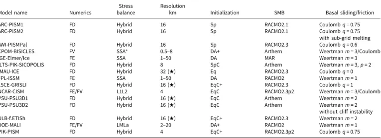
Table 2.List of ABUMIP simulations and main model characteristics Stress Resolution
Model name Numerics balance km Initialization SMB Basal sliding/friction ARC-PISM1 FD Hybrid 16 Sp RACMO2.1 Coulomb q = 0.75 ARC-PISM2 FD Hybrid 16 Sp RACMO2.1 Coulomb q = 0.75
with sub-grid melting AWI-PISMPal FD Hybrid 16 Sp RACMO2.3 Coulomb q = 0.6 CPOM-BISICLES FV SSA∗ 0.5–8 DA+ Arthern Weertman m = 3/Coulomb IGE-Elmer/Ice FE SSA 1–50 DA MAR Weertman m = 3 ILTS-PIK-SICOPOLIS FD Hybrid 8 SpC Arthern Weertman m = 3, p = 2 IMAU-ICE FD Hybrid 32 (w) Eq RACMO2.3 Coulomb q = 0 JPL-ISSM FE SSA 1–50 DA RACMO2 Weertman m = 1 LSCE-GRISLI FD Hybrid 16 (w) EqC+ RACMO2.3 Coulomb q = 1
NCAR-CISM FE/FV L1L2 4 EqC RACMO2.3p2 Weertman m = 3/Coulomb PSU-PSU3D1 FD Hybrid 16 (w) EqC Arthern Weertman m = 2 PSU-PSU3D2 FD Hybrid 16 (w) EqC Arthern Weertman m = 2
without cliff instability ULB-f.ETISh FD Hybrid 16 (w) EqC+ RACMO2.3 Weertman m = 2 DOE-MALI FE/FV LMLa 2–20 DA+ RACMO2 Weertman m = 1 PIK-PISM FD Hybrid 4 EqC+ RACMO2.3p2 Coulomb q = 0.75
Numerics rely on the finite-difference (FD), finite-element (FE) or finite-volume (FV) method. Stress balance approximations implemented by models include Shallow-Shelf Approximation (SSA; see MacAyeal,1989), SSA with vertical shear terms represented in the effective viscosity term (SSA*; see Cornford and others,2013), combination of SSA and Shallow-Ice Approximation (Hybrid; see Bueler and Brown,2009; Winkelmann and others,2011), depth-integrated higher-order approximation (L1L2; see Goldberg,2011) and Blatter–Pattyn approximation (LMLa; see Pattyn,2003). Initialization methods are as follows: spin-up (Sp), spin-up with target values for the ice thickness (SpC), data assimilation (DA), equilibrium state (Eq) and equilibrium state with target values for the ice thickness (EqC; see Pollard and DeConto,2012a). (+) Means relaxation after initialization. (w) Marks models that use a grounding line flux parameterization (e.g. Pollard and DeConto,2012a). Initial SMB is derived from the following: RACMO2 (Lenaerts and others,2012), RACMO2.3 (Van Wessem and others,2014), RACMO2.3p2 (Van Wessem and others,
2018), MAR (Agosta and others,2019) and Arthern and others (2006) (Arthern). Ice-sheet geometries are based on Bedmachine (Morlighem and others,2020) for f.ETISh and Bedmap2 (Fretwell and others,2013) for all other models. Further details on all the models are given in the Appendix.
Fig. 1.Volume above flotation (in m SLE) and contribution to sea-level rise (SLR) for ABUC (left) and both ABUK and ABUM experiments (positive means higher sea-level contribution). Subplots b, c and d with title‘-INIT’ represent the sea-level contribution compared to the initial state.
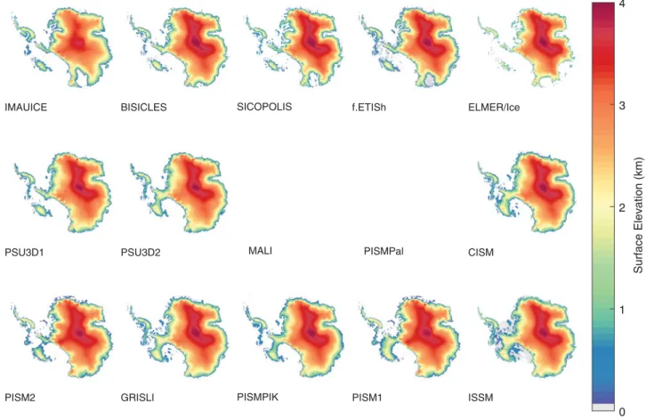
Fig. 2.Surface elevation for the grounded ice sheet after 500 years in ABUK for all participating models. The sequence of models is ordered from lowest to highest grounded area at the end of the simulations. All models effectively lose a large part of WAIS. Some models also lose mass in Recovery Subglacial Basin, Wilkes Subglacial Basin and Aurora Subglacial Basin.
In a spatial context, this implies that all models effectively lose the West Antarctic ice sheet (WAIS) or at least a large part of it (Figs 2 and 3). One exception is ARC-PISM1 with little grounding line retreat in Thwaites glacier, which may be due to a too-coarse spatial resolution across the grounding line (Gladstone and others, 2010, 2012; Pattyn and others, 2013; Leguy and others, 2014). The use of sub-shelf melting under-neath grounded parts of the ice-sheet results in higher mass loss with that same model, as shown by the results of ARC-PISM2. PIK-PISM and LSCE-GRISLI conserve an ice bridge in the centre of the WAIS at the end of both experiments, while JPL-ISSM, CISM and PSU3D2 maintain the ice bridge in ABUM experiment.
The ABUK experiment also allows to identify potential mass loss due to MISI. For instance, Bamber and others (2009) calcu-late the potential contribution to SLR due to WAIS collapse with a simple method: they identify grid cells below sea level on retro-grade bed slopes to infer the limit of grounding-line retreat, which leads to a SLR contribution of 3.3 m. However, in order to fully capture the effect of MISI, all dynamical effects need to be taken into account, which is only possible using marine ice-sheet models. ABUK provides such a multi-model experiment in which ice-shelf buttressing is completely removed and the modelled ice sheet evolves through MISI. Most participating mod-els therefore simulate a collapse of the WAIS. In order to make comparison with Bamber and others (2009) possible, we recalcu-lated the mass loss for the same WAIS area. For ABUK, this ranges from 1.91 to 5.08 m, with a mean value of 3.16 m SLE. When considering only those models that are reproducing a full collapse of WAIS, this ranges from 2.86 to 5.08 m, with a mean value of 3.67 m SLE, which is higher than the value given in Bamber and others (2009).
Multi-metre ice mass loss beyond 2–3 m SLE is related to loss of grounded ice in sectors of the East Antarctic ice sheet (EAIS), especially in Recovery Subglacial Basin (location shown in Fig. 4). Some models also lose mass in Wilkes Subglacial Basin and to a lesser extent Aurora Subglacial Basin (locations shown in Fig. 4), i.e. IMAU-ICE, ILTS-PIK-SICOPOLIS, ULB-f.ETISh, IGE-Elmer/Ice and CPOM-BISICLES (Fig. 2).
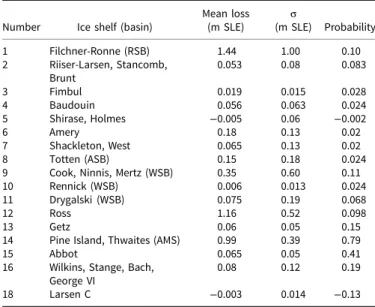
The overall assessment of the response of the different models is described by the mean value of the average percentage of ice-thickness change against the initial ice thickness over the model ensemble (probability) and its standard deviation among the participating models (Fig. 4). For specific basins, the mean mass loss, the standard deviation of mass loss and the mean pro-portion of mass loss are listed inTable. 3. The highest values of mass loss occur in the Recovery Subglacial Basin (1.44 m SLE) due to the loss of the Filchner-Ronne ice shelf, in the Siple Coast ice streams (1.16 m SLE) due to the loss of the Ross ice shelf, and in the Amundsen Sea Embayment due to the loss of the Thwaites and Pine Island Glaciers (0.99 m SLE). The standard deviation in the Recovery Subglacial Basin is also high, meaning that models agree less in this basin, while most models agree on the amount of mass loss in the Siple Coast and Amundsen Sea Embayment. The central part of the WAIS has a lower probability of mass loss, since not all models exhibit a complete collapse of the WAIS. The lowest probability and highest standard deviation are seen for the Wilkes and Aurora Subglacial Basins in East Antarctica, as only few models exhibit mass loss in those sectors.
ABUM
The ABUM experiment shows similar characteristics as ABUK, except IGE-Elmer/Ice where ABUM has the most mass loss (up
Fig. 3.Surface elevation for the grounded ice sheet after 500 years in experiment ABUM for all participating models. Similar to ABUK results, all models effectively lose a large part of WAIS. Some models also lose mass in Recovery Subglacial Basin, Wilkes Subglacial Basin and Aurora Subglacial Basin. The sequence of the model results is the same as inFigure 2to facilitate the comparison.
to 12 m SLE after 500 years). This is likely a mesh resolution issue in the model, as the grounding line migrates beyond the refined grid into the coarser grid areas in ABUM, while the domain was remeshed every 5 years in the ABUK experiment.
It is also interesting to note that PSU3D1 that includes cliff collapse, does not differ that much from the results of PSU3D2, without the cliff collapse mechanism activated. The reason behind the difference with results from Pollard and others (2015); DeConto and Pollard (2016) lies in the fact that surface melt is necessary to provoke hydro-fracturing of the grounded ice sheet to initiate cliff collapse, and this surface melt is not large enough in the current experimental set up. Since the ABUK and ABUM experiment lack any atmospheric forcing, cliff collapse is not invoked by hydro-fracture process.
Discussion
Sensitivity to basal friction
In the ensemble of model results, there seems to be a general ten-dency of increased mass loss with increased plasticity of the fric-tion law, both Weertman and Coulomb (Fig. 5, where the different models are grouped according to basal friction law). For the ABUK experiment results, models implementing linear Weertman/Coulomb friction law result in 3.07 m SLE ice loss on average, while the value for the pseudo-plastic Coulomb fric-tion law, the Weertman fricfric-tion law with m = [2, 3], and the plas-tic Coulomb friction law are 4.41, 5.10, 4.95 and 10.20 m SLE, respectively. The same trend is shown in ABUM experiment results; models implementing the linear Weertman/Coulomb
friction law result in 1.49 m SLE ice loss on average, while the value for the pseudo-plastic Coulomb friction law, the Weertman friction law with m = [2, 3], and the plastic Coulomb friction law are respectively 4.41, 4.81, 7.02 and 10.08 m SLE. In the subgroup of pseudo-plastic Coulomb friction law, where dif-ferent branches of the PISM model are implemented, a ‘more’ plastic sliding law with q = 0.6 results in larger mass loss com-pared to those with q = 0.75. However, this trend is not straight-forward for all of the models. This means that other factors influence the model sensitivity as well, and they most likely pertain to differences in numerical approaches of the models, especially the spatial resolution across the grounding line and the way models simulate grounding line migration (Gladstone and others, 2010, 2012; Pattyn and others, 2012, 2013; Pattyn and Durand,2013; Leguy and others,2014; Durand and Pattyn, 2015; Brondex and others,2017). This is further detailed below.
The response to a sudden removal of ice shelves for the differ-ent models is not clearly related to the initialization method. However, as also shown in Joughin and others (2009); Parizek and others (2013); Brondex and others (2017); Pattyn (2017); Brondex and others (2019) and Bulthuis and others (2019), plastic sliding/friction law generally lead to more prominent grounding-line migration compared to viscous sliding laws. To demonstrate this, we performed the ABUK experiment with one model (ULB-f.ETISh) for a Weertman sliding law with exponents m = 1, 2, 3, 4, and for the Coulomb friction law with q = 1 (linear case). Figure 6demonstrates that a viscous sliding law is the least sensi-tive to mass loss due to a sudden and sustained loss of ice shelves; the amount of mass loss increases with increasing exponent m. The highest mass loss is encountered for the linear Coulomb
Fig. 4.Average percentage of thickness change against the initial ice thickness over the model ensemble (left column) after 500 years for the ABUK (top) and ABUM (bottom) models. Standard deviation of the percentage of thickness change (right column). Major place names and subglacial basin numbers ofTable 3of the Antarctic Ice Sheet are given in the different panels (AMS, Amundsen Sea Sector; WSB, Wilkes Subglacial Basin; ASB, Aurora Subglacial Basin; RSB, Recovery Subglacial Basin; EAIS, East Antarctic Ice Sheet; WAIS, West Antarctic Ice Sheet).
Fig. 5.Overall mass loss (volume above flotation; VAF) for the participating models ordered according to basal friction law characteristics: Weertman and Coulomb linear (m = 1, q = 1), pseudo-plastic Coulomb (q= 0.6--0.75), Weertman m = 2, Weertman m = 3, Coulomb plastic q = 0. Models that did not participate a particular experiment are marked by‘X’.
Fig. 6.Ice mass loss for the ABUK and ABUC (labelled) experiments with ULB-f.ETISh for different exponents of the Weertman law (m = 1, 2, 3, 4) and the linear Coulomb friction law (CF, q = 1). The amount of mass loss increases with increasing exponent m.
friction case. However, different grounding line flux parameteri-zations are implemented in the ULB-f.ETISh model depending on the sliding laws. Indeed, a Coulomb friction law implies a zero effective pressure N at the grounding line (Leguy and others, 2014; Tsai and others,2015), which leads to a higher sensitivity compared to the parameterization due to Schoof (2007) and demonstrated in Pattyn (2017).
Sensitivity to the forcing scheme
Most models have a slightly higher mass loss after 500 years for the ABUK than for the ABUM experiment (Fig. 5) due to the remaining weak buttressing from ice shelves in the latter. However, some models show a suspiciously stronger sensitivity for ABUM compared to ABUK although the ice-shelf removal should intrinsically have a stronger effect than applying excessive sub-shelf melt rates.
The reason for the more pronounced mass loss in IGE-Elmer/ Ice stems from the difference in numerical set up for both experi-ments. Initially the mesh is much finer mesh around the grounding line and coarser inland. While a new mesh is generated every 5 years to cope with grounding-line retreat in ABUK, the ABUM experiment considers a fixed mesh, so that the grounding line irre-vocally retreats from a mesh of 1 to 32 km during the model run. There are few other models ARC-PISM1, ARC-PISM2, PISM-PIK, ILTS-PIK-SICOPOLIS with higher mass loss for ABUM to a less extent, from 0.82 to 1.9 m SLE. A possible explan-ation is that the sliding scheme in the vicinity of the grounding line is interpolated as a function of surface gradients and driving stress (Feldmann and others,2014; Gladstone and others,2017) so as to have a continuous transition of sliding from the ground-ing zone to the floatground-ing zone. The presence of floatground-ing ice in ABUM leads to a gentler surface gradient, and therefore higher sliding at the grounding line compared to ABUK where the grounding line acts as a computational boundary.
Sensitivity to model physics and numerics
The sensitivity of the experimental results to model physics and numerics is more difficult to assess. We considered several
essential factors: spatial resolution, initial ice and bedrock geom-etry, basal sliding law and subglacial hydrology.
Spatial resolution
Spatial resolution may have a profound impact as previous assess-ments on marine ice-sheet models have demonstrated (Pattyn and others,2012,2013; Leguy and others,2014). Comparing numer-ical models to theory (Schoof, 2007), Pattyn and others (2012) showed that a spatial resolution of <1 km is necessary to capture the essential dynamics of grounding lines. However, the grid size is also dependent on the basal friction transition across the grounding line, i.e. for a sharp contrast of no slip (grounded ice sheet) to free slip (ice shelf), spatial resolution needs to be high, but smoother transitions– e.g. from a weak till-based ice stream to an ice shelf – are more forgiving with respect to resolution (Pattyn and others, 2006; Gladstone and others, 2010, 2012; Leguy and others,2014). Moreover, sub-grid grounding line inter-polations also relax some resolution requirements (Parizek and others, 2013; Seroussi and others, 2014; Cornford and others, 2016; Hoffman and others, 2018) and such parameterizations are applied in DOE-MALI, NCAR-CISM, ARC-PISM, AWI-PISMPal and PIK-PISM. Some models apply an analytic con-straint on the flux across the grounding line based on theoretical derivations for an unbuttressed flow-line setting (e.g. Schoof, 2007). This is the case for IMAU-ICE, LSCE-GRISLI, PSU-PSU3D and ULB-f.ETISh.
High-resolution models without grounding-line parameteriza-tions, interpolations or heuristics, such as DOE-MALI, IGE-Elmer/Ice and CPOM-BISICLES, produce ice mass loss in the range of 3.5–5 m SLE after 500 years. They corroborate results of the other models, i.e. that they lose the complete WAIS and parts of the Recovery and Wilkes Subglacial Basins. However, this sample is too small to confirm whether these mass loss bounds can be considered as being representative of the highest resolution models.
Apart from models with mesh refinement schemes, most of models implement 16 km resolution in the simulations. Models with 4 km resolution (PIK-PISM and CISM) have less mass loss compared to models with similar sliding laws (Fig. 5). IMAU-ICE has the coarsest resolution of 32 km as well as the highest mass loss especially in Wilkes Subglacial Basin. While IMAU-ICE is the only model with 32 km resolution and the only model with Coulomb plastic sliding law, the high mass loss could therefore be a result of the combination of both.
Initial geometry
Other differences may be due to the initial conditions applied in the models, such as the initial surface and bed topography (ULB-f.ETISh used BedMachine Antarctica (Morlighem and others, 2020) while all other models used Bedmap2 (Fretwell and others,2013)).
Basal sliding law
The tendency for increased model sensitivity to the power of the sliding law, as demonstrated inFigure 6, is only marginally clear when grouping the models in a similar way (Fig. 5). This means that the level of noise, due to different numeric approaches, spatial resolutions, model physics and boundary conditions in the ensemble, is of comparable order of magnitude as the signal.
Subglacial hydrology
A major uncertainty remains in the physical understanding and modelling of subglacial till mechanics that are essential for deter-mining the effective pressure and sliding rate at the base of a marine ice sheet. The few studies that have attempted to tackle this problem (e.g. Bueler and van Pelt, 2015; Gladstone and
Table 3. Model results of mass loss for Antarctic subglacial basins after 500-year simulation of ABUK
Number Ice shelf (basin)
Mean loss (m SLE) σ (m SLE) Probability 1 Filchner-Ronne (RSB) 1.44 1.00 0.10 2 Riiser-Larsen, Stancomb, Brunt 0.053 0.08 0.083 3 Fimbul 0.019 0.015 0.028 4 Baudouin 0.056 0.063 0.024 5 Shirase, Holmes −0.005 0.06 −0.002 6 Amery 0.18 0.13 0.02 7 Shackleton, West 0.065 0.13 0.02 8 Totten (ASB) 0.15 0.18 0.024 9 Cook, Ninnis, Mertz (WSB) 0.35 0.60 0.11 10 Rennick (WSB) 0.006 0.013 0.024 11 Drygalski (WSB) 0.075 0.19 0.068 12 Ross 1.16 0.52 0.098 13 Getz 0.06 0.05 0.15 14 Pine Island, Thwaites (AMS) 0.99 0.39 0.79 15 Abbot 0.065 0.05 0.41 16 Wilkins, Stange, Bach,
George VI
0.08 0.12 0.19 18 Larsen C −0.003 0.014 −0.13
Basin numbers are in accordance with Reese and others (2018a).σ is the standard deviation of mean mass loss in the basin. Probability is the average percentage of mass loss against the initial mass of the basin over the model ensemble. Present-day basin boundaries are used, without consideration of divide migration during the simulation. The abbreviations of the basins are the same withFigure 4.
others,2017) are based on seminal work by Tulaczyk and others (2000a, 2000b), but it is clear that more research in subglacial hydrology and basal mechanics of marine ice sheets is needed.
New techniques have been and will need to be further explored to improve initialization methods using both observed surface elevation and ice velocity changes, allowing for improved under-standing of underlying friction laws and rheological conditions of marine-terminating glaciers (Gillet-Chaulet and others, 2016; Gillet-Chaulet,2020). Observations in regions with large changes can be used to discriminate different parameterizations. Joughin and others (2009), Joughin and others (2019) and Gillet-Chaulet and others (2016) have shown that plastic laws are better suited for fast flowing areas in Pine Island Glacier in the Amundsen Sea Embayment, which in the light of this study makes a strong case for the increased sensitivity of grounding-line retreat and ice-sheet response relative to the commonly used slid-ing laws. Transient data assimilation (Goldberg and others,2015; Gillet-Chaulet, 2020) that allow to capture observed rates of change should give better confidence in projections and enable reanalysis to better comprehend processes that drive past changes.
Sensitivity to hydro-fracturing and Marine Ice Cliff Instability
The Marine Ice Cliff Instability (MICI) mechanism (based on Bassis and Walker, 2012; DeConto and Pollard, 2016 and Pollard and others,2015) leads to SLR projections exceeding 12 m after 500 years for unmitigated climate scenarios. This value is out-side the range of most of the projections (Hanna and others,2020), but not that far out of the range of the upper end model results with the ABUMIP ensemble and without MICI. This demonstrates that other processes besides the MICI may result in large mass loss from the Antarctic ice sheet, including marine basins from the EAIS, and still match values representative of Pliocene sea-level high stands (Edwards and others,2019). Plastic Coulomb friction laws in par-ticular increase the sensitivity of grounding-line retreat under reduced ice-shelf buttressing. The inclusion of hydro-fracturing in PSU-PSU3D1 results in ∼1.5 m SLE higher mass loss in the ABUK and ABUM experiments compared to the PSU-PSU3D2 model without the extra physics. This lack of considerable mass loss compared to DeConto and Pollard (2016) is mainly due to the absence of atmospheric anomalies in ABUMIP that otherwise would produce substantial surface melt to initiate the hydro-fracturing process.
Comparison to other studies
Three recent studies (Fürst and others, 2016; Reese and others, 2018b; Gudmundsson and others,2019) investigated the sensitiv-ity of ice shelves to buttressing on the inland ice sheet. However, all of them investigated the current and immediate impact of ice shelves on the buttressing potential, not attempting to quantify buttressing importance as a function of potential ice mass loss over time. Martin and others (2019) quantified the vulnerability of present-day Antarctic ice sheet to regional ice-shelf collapse on millennial timescales using BISICLES. ABUMIP therefore offers a unique opportunity to quantify the potential mass loss for the extreme case where all ice shelves are lost and gauges the response of the ice sheet to such dramatic collapse.
The ABUM experiment is comparable to the M3 experiment from the SeaRISE project (Bindschadler and others, 2013; Nowicki and others,2013) that considered extreme sub-ice-shelf melting with a lower melt rate of 200 m a−1. Despite the higher sub-ice-shelf melting implemented by ABUM, the range of mass loss is significantly decreased from [2–20] m SLE in SeaRISE com-pared to [1–12] m SLE in ABUM. The better agreement between models here is due to the fact that (i) ice streams are better resolved
(in terms of spatial resolution and/or model physics that all include membrane stresses), and (ii) grounding line dynamics are better captured (e.g. Pattyn and others, 2013; Leguy and others, 2014; Durand and Pattyn,2015). All models now allow for the grounding line to migrate, either through the use of a finer mesh or by means of grounding-line flux parameterizations. Furthermore, ice-sheet models include dynamic ice shelves, which was not the case with the SeaRISE ensemble. Some models in that specific ensemble applied sub-shelf melting spread out across grounded cells, which increases the sensitivity to sub-shelf melt forcing of the model through enhanced grounding-line retreat (Durand and Pattyn, 2015; Seroussi and Morlighem,2018).
Conclusions
We have presented results of the ISMIP6-ABUMIP experiment that investigate the effects of a sudden loss of ice shelves on Antarctic ice sheet volume change, either through a complete and sustained collapse of ice shelves (ABUK) or an extreme sub-shelf melting rate (ABUM). Results of both experiments exhibit similar responses, i.e. a fast response and high probability of com-plete collapse of the WAIS and potential gradual mass loss of some EAIS basins, such as Recovery, Wilkes subglacial basins and to a lesser extent Aurora subglacial basin. Previous studies estimated the WAIS collapse due to MISI as 3.3 m SLE (Bamber and others, 2009). Our study shows that WAIS collapse poten-tially leads to a 1.91–5.08 m sea level rise when ice-dynamical effects are included.
In the absence of ice-shelf buttressing, simulated mass losses are evidently controlled primarily by basal conditions. Basal fric-tion laws with a higher plasticity lead to a more sensitive response to reduced ice-shelf buttressing. The effect of plasticity in a basal friction law (m = 4 vs m = 1 in a Weertman sliding law) alone causes a ∼7 m SLE difference for the ABUK experiment. Gillet-Chaulet and others (2016) suggest that a more plastic slid-ing law m≥5 is required to accurately reproduce the observed acceleration in fast flowing regions. If plastic sliding laws are more applicable Antarctic-wide, the ice sheet will have higher sen-sitivity to ice-shelf loss of buttressing. The range of mass loss indi-cates that processes other than the Marine Ice Cliff Instability are capable of reproducing large mass losses over centennial time spans, similar to inferred Pliocene sea-level high stands. Given the importance of subglacial processes in guiding the rate of mass loss of marine basins, the inclusion of a more realistic sub-glacial hydrology will be another challenge for the ice-sheet mod-elling community.
Uncertainties also stem from numerical approximations, such as spatial and temporal resolutions of the model, as well as param-eterization methods for physical processes operating at the grounding line. However, the relatively small ensemble of models with diverse methods make it difficult to quantify the uncertain-ties from different schemes. Sensitivity tests of different schemes within a single model would therefore be of particular interest. This study will help to better understand the spread in projections of 21st century Antarctic ice sheet contributions to sea level.
Data availability
The model output from the simulations described in this paper and forcing data sets will be made publicly available with digital object identifier https://doi.org/10.5281/zenodo.3932935. In order to document CMIP6’s scientific impact and enable ongoing support of CMIP, users are asked to acknowledge CMIP6, ISMIP6 and the participating modelling groups.
Acknowledgments. We thank the Climate and Cryosphere (CliC) effort, which provided support for ISMIP6 through sponsoring of workshops, hosting the ISMIP6 website and wiki, and promoted ISMIP6. We acknowledge the World Climate Research Programme, which, through its Working Group on Coupled Modelling, coordinated and promoted CMIP5 and CMIP6. We thank the climate modelling groups for producing and making available their model output, the Earth System Grid Federation (ESGF) for archiving the CMIP data and providing access, the University at Buffalo for ISMIP6 data distribution and upload, and the multiple funding agencies who support CMIP5 and CMIP6 and ESGF. Support for Matthew Hoffman, Stephen Price and Tong Zhang was provided through the Scientific Discovery through Advanced Computing (SciDAC) programme funded by the US Department of Energy (DOE), Office of Science, Advanced Scientific Computing Research and Biological and Environmental Research Programs. MALI simu-lations used resources of the National Energy Research Scientific Computing Center, a DOE Office of Science user facility supported by the Office of Science of the US Department of Energy under Contract DE-AC02-05CH11231. Ralf Greve was supported by the Japan Society for the Promotion of Science (JSPS) KAKENHI grant numbers JP16H02224, JP17H06104 and JP17H06323. Support for Mathieu Morlighem was provided by the National Science Foundation (NSF: Grant 1739031). The work of Thomas Kleiner has been conducted in the framework of the PalMod project (FKZ: 01LP1511B), supported by the German Federal Ministry of Education and Research (BMBF) as Research for Sustainability initiative (FONA). Reinhard Calov was funded by the PalMod project (PalMod 1.1 and 1.3 with grants 01LP1502C and 01LP1504D) of the German Federal Ministry of Education and Research (BMBF). Johannes Sutter has been funded via the AWI Strategy Fund and the regional climate initiative REKLIM. Tanja Schlemm is funded by a doctoral stipend granted by the Heinrich Böll Foundation. Torsten Albrecht has been funded by the Deutsche Forschungsgemeinschaft (DFG) in the framework of the priority programme ‘Antarctic Research with comparative investigations in Arctic ice areas’ by grant WI4556/2-1 and WI4556/4-1. Hélène Seroussi, Erika Simon and Sophie Nowicki were supported by grants from NASA Cryospheric Science and Modeling, Analysis, Predictions Programs. Computing resources support-ing ISSM simulations were provided by the NASA High-End Computsupport-ing Program through the NASA Advanced Supercomputing Division at Ames Research Center. Gunter Leguy and William Lipscomb were supported by the National Center for Atmospheric Research, which is a major facility spon-sored by the National Science Foundation under Cooperative Agreement No. 1852977. Computing and data storage resources supporting CISM, including the Cheyenne supercomputer (doi:10.5065/D6RX99HX), were provided by the Computational and Information Systems Laboratory (CISL) at NCAR. Heiko Goelzer has received funding from the programme of the Netherlands Earth System Science Centre (NESSC), financially supported by the Dutch Ministry of Education, Culture and Science (OCW) under grant no. 024.002.001. This research forms part of the MIMO project within the STEREO III programme of the Belgian Science Policy Office, contract SR/ 00/336. IGE-Elmer/Ice simulations were performed using HPC resources from GENCI-CINES (grant 2018-016066) and using the Froggy platform of the CIMENT infrastructure, which is supported by the Rhone-Alpes region (grant CPER07_13 CIRA), the OSUG@2020 laBex (reference ANR10 LABX56) and the Equip@Meso project (referenceANR-10-EQPX-29-01). Nicholas R. Golledge acknowledges funding from Royal Society of New Zealand grant RDF-VUW1501. This is ISMIP6 contribution 14.
Author contributions.
S.S., F.P. and N.G. designed and coordinated the study, S.S. and F.P. led the writing, E.G.S. and S.S. processed the data and all authors contributed to the experiments, writing and discussion of ideas.
References
Agosta C, Amory C, Kittel C, Orsi A, Favier Vand 6 others (2019) Estimation of the Antarctic surface mass balance using the regional climate model MAR (1979–2015) and identification of dominant processes. The Cryosphere 13(1), 281–296. doi:10.5194/tc-13-281-2019.
Albrecht T, Winkelmann R and Levermann A(2020) Glacial-cycle simulations of the Antarctic Ice Sheet with the Parallel Ice Sheet Model (PISM)– Part 1: boundary conditions and climatic forcing. The Cryosphere 14(2), 599–632. doi:10.5194/tc-14-599-2020.
Alley RB and 7 others (2015) Oceanic forcing of ice-sheet retreat: West Antarctica and more. Annual Review of Earth and Planetary Sciences 43 (1), 207–231. doi:10.1146/annurev-earth-060614-105344.
Arthern RJ, Winebrenner DP and Vaughan DG(2006) Antarctic snow accu-mulation mapped using polarization of 4.3-cm wavelength microwave emis-sion. Journal of Geophysical Research: Atmospheres 111, D06107, doi:10. 1029/2004JD005667.
Aschwanden A and 7 others(2019) Contribution of the Greenland Ice Sheet to sea level over the next millennium. Science Advances 5(6), eaav9396, doi:
10.1126/sciadv.aav9396.
Aschwanden A, Adalgeirsdóttir G and Khroulev C(2013) Hindcasting to measure ice sheet model sensitivity to initial states. The Cryosphere 7(4), 1083–1093. doi:10.5194/tc-7-1083-2013.
Aschwanden A, Bueler E, Khroulev C and Blatter H(2012) An enthalpy for-mulation for glaciers and ice sheets. Journal of Glaciology 58(209), 441–457. doi:10.3189/2012JoG11J088.
Bamber JL, Riva REM, Vermeersen BLA and LeBrocq AM (2009) Reassessment of the potential sea-level rise from a collapse of the West Antarctic ice sheet. Science 324(5929), 901–903. doi:10.1126/science.1169335. Bassis JN and Walker CC(2012) Upper and lower limits on the stability of calving glaciers from the yield strength envelope of ice. Proceedings of the Royal Society A: Mathematical, Physical and Engineering Sciences 468 (2140), 913–931. doi:10.1098/rspa.2011.0422.
Bernales J, Rogozhina I, Greve R and Thomas M(2017) Comparison of hybrid schemes for the combination of shallow approximations in numer-ical simulations of the Antarctic Ice Sheet. The Cryosphere 11(1), 247–265. doi:10.5194/tc-11-247-2017.
Bindschadler RA and 27 others(2013) Ice-sheet model sensitivities to envir-onmental forcing and their use in projecting future sea level (the SeaRISE project). Journal of Glaciology 59(214), 195–224. doi: 10.3189/ 2013JoG12J125.
Blatter H(1995) Velocity and stress fields in grounded glaciers: a simple algo-rithm for including deviatoric stress gradients. Journal of Glaciology 41 (138), 333–344. doi:10.3189/S002214300001621X.
Brondex J, Gagliardini O, Gillet-Chaulet F and Durand G(2017) Sensitivity of grounding line dynamics to the choice of the friction law. Journal of Glaciology 63(241), 854–866. doi:10.1017/jog.2017.51.
Brondex J, Gillet-Chaulet F and Gagliardini O(2019) Sensitivity of centen-nial mass loss projections of the Amundsen basin to the friction law. The Cryosphere 13(1), 177–195. doi:10.5194/tc-13-177-2019.
Bueler E and Brown J(2009) Shallow shelf approximation as a‘sliding law’ in a thermomechanically coupled ice sheet model. Journal of Geophysical Research: Earth Surface 114(F3), F03008. doi:10.1029/2008JF001179. Bueler E and van Pelt W(2015) Mass-conserving subglacial hydrology in the
Parallel Ice Sheet Model version 0.6. Geoscientific Model Development 8(6), 1613–1635. doi:10.5194/gmd-8-1613-2015.
Bulthuis K, Arnst M, Sun S and Pattyn F(2019) Uncertainty quantification of the multi-centennial response of the Antarctic ice sheet to climate change. The Cryosphere 13(4), 1349–1380. doi:10.5194/tc-13-1349-2019. Calov R and 8 others(2018) Simulation of the future sea level contribution of
Greenland with a new glacial system model. The Cryosphere 12(10), 3097– 3121. doi:10.5194/tc-12-3097-2018.
Cornford SL and 8 others(2013) Adaptive mesh, finite volume modeling of marine ice sheets. Journal of Computational Physics 232, 529–549. Cornford SL, Martin DF, Lee V, Payne AJ and Ng EG (2016) Adaptive
mesh refinement versus subgrid friction interpolation in simulations of Antarctic ice dynamics. Annals of Glaciology 57(73), 1–9. doi:10.1017/ aog.2016.13.
DeConto RM and Pollard D(2016) Contribution of Antarctica to past and future sea-level rise. Nature 531(7596), 591–597. doi:10.1038/nature17145. Durand G and Pattyn F (2015) Reducing uncertainties in projections of Antarctic ice mass loss. The Cryosphere 9(6), 2043–2055. doi:10.5194/ tc-9-2043-2015.
Edwards TL and 9 others(2019) Revisiting Antarctic ice loss due to marine ice-cliff instability. Nature 566(7742), 58–64. doi: 10.1038/ s41586-019-0901-4.
Favier L and 7 others(2019) Assessment of sub-shelf melting parameterisa-tions using the ocean–ice-sheet coupled model nemo(v3.6)–elmer/ice (v8.3). Geosci. Model Dev. 12, 2255–2283. doi:10.5194/gmd-12-2255-2019. Feldmann J, Albrecht T, Khroulev C, Pattyn F and Levermann A(2014) Resolution-dependent performance of grounding line motion in a shallow model compared with a full-Stokes model according to the MISMIP3d
intercomparison. Journal of Glaciology 60(220), 353–360. doi: 10.3189/ 2014JoG13J093.
Fortuin JPF and Oerlemans J(1990) Parameterization of the annual surface temperature and mass balance of Antarctica. Annals of Glaciology 14, 78– 84. doi:10.3189/S0260305500008302.
Fretwell P and 59 others(2013) Bedmap2: improved ice bed, surface and thickness datasets for Antarctica. The Cryosphere 7(1), 375–393. doi:10. 5194/tc-7-375-2013.
Fürst JJ and 6 others(2016) The safety band of Antarctic ice shelves. Nature Climate Change 6(5), 479–482. doi:10.1038/nclimate2912.
Gillet-Chaulet F and 6 others (2016) Assimilation of surface velocities acquired between 1996 and 2010 to constrain the form of the basal friction law under Pine Island Glacier. Geophysical Research Letters 43(19), 10311– 10321. doi:10.1002/2016GL069937.
Gillet-Chaulet F(2020) Assimilation of surface observations in a transient marine ice sheet model using an ensemble Kalman filter. The Cryosphere 14(3), 811–832. doi:10.5194/tc-14-811-2020.
Gladstone RM and 5 others(2017) Marine ice sheet model performance depends on basal sliding physics and sub-shelf melting. The Cryosphere 11(1), 319–329. doi:10.5194/tc-11-319-2017.
Gladstone RM, Payne AJ and Cornford SL (2010) Parameterising the grounding line in ice sheet models. The Cryosphere 4(4), 605–619. doi:
10.5194/tc-4-605-2010.
Gladstone RM, Payne AJ and Cornford SL(2012) Resolution requirements for grounding-line modelling: sensitivity to basal drag and ice-shelf buttres-sing. Annals of Glaciology 53(60), 97–105. doi:10.3189/2012AoG60A148. Goelzer H and 30 others(2018) Design and results of the ice sheet model
ini-tialisation experiments initMIP-Greenland: an ISMIP6 intercomparison. The Cryosphere 12(4), 1433–1460. doi:10.5194/tc-12-1433-2018. Goldberg DN(2011) A variationally derived, depth-integrated approximation
to a higher-order glaciological flow model. Journal of Glaciology 57(201), 157–170. doi:10.3189/002214311795306763.
Goldberg DN, Heimbach P, Joughin I and Smith B (2015) Committed retreat of Smith, Pope, and Kohler Glaciers over the next 30 years inferred by transient model calibration. The Cryosphere 9(6), 2429–2446. doi:10. 5194/tc-9-2429-2015.
Golledge NR and 6 others(2019) Global environmental consequences of twenty-first-century ice-sheet melt. Nature 566(7742), 65–72. doi: 10. 1038/s41586-019-0889-9.
Golledge NR, Levy RH, McKay RM and Naish TR(2017) East Antarctic ice sheet most vulnerable to Weddell Sea warming. Geophysical Research Letters 44(5), 2343–2351. doi:10.1002/2016GL072422.
Grant GR and 9 others(2019) The amplitude and origin of sea-level variabil-ity during the Pliocene epoch. Nature 574(7777), 237–241. doi:10.1038/ s41586-019-1619-z.
Greve R and SICOPOLIS Developer Team(2019) SICOPOLIS v5.1. Zenodo. doi:10.5281/zenodo.3727511
Greve R and Blatter H(2016) Comparison of thermodynamics solvers in the polythermal ice sheet model SICOPOLIS. Polar Science 10(1), 11–23. doi:
10.1016/j.polar.2015.12.004.
Gudmundsson GH, Paolo FS, Adusumilli S and Fricker HA (2019) Instantaneous Antarctic ice sheet mass loss driven by thinning ice shelves. Geophysical Research Letters 46(23), 13903–13909. doi: 10.1029/ 2019GL085027.
Hanna E and 10 others(2020) Mass balance of the ice sheets and glaciers– progress since AR5 and challenges. Earth-Science Reviews 201, 102976. doi:
10.1016/j.earscirev.2019.102976..
Hoffman MJ and 9 others(2018) MPAS-Albany Land Ice (MALI): a variable-resolution ice sheet model for Earth system modeling using Voronoi grids. Geoscientific Model Development 11(9), 3747–3780. doi: 10.5194/ gmd-11-3747-2018.
Jenkins A and 6 others(2010) Observations beneath Pine Island Glacier in West Antarctica and implications for its retreat. Nature Geoscience 3(7), 468–472. doi:10.1038/ngeo890.
Jenkins A and 7 others (2018) West Antarctic Ice Sheet retreat in the Amundsen Sea driven by decadal oceanic variability. Nature Geoscience 11(10), 733–738. doi:10.1038/s41561-018-0207-4.
Joughin IR and 6 others(2009) Basal conditions for Pine Island and Thwaites Glaciers, West Antarctica, determined using satellite and airborne data. Journal of Glaciology 55(190), 245–257. doi:10.3189/002214309788608705. Joughin I, Smith BE and Schoof CG(2019) Regularized coulomb friction laws for ice sheet sliding: application to pine island glacier, antarctica.
Geophysical Research Letters 46(9), 4764–4771. doi: 10.1029/ 2019GL082526.
Jourdain NC and 6 others(2019) A protocol for calculating basal melt rates in the ISMIP6 Antarctic ice sheet projections. The Cryosphere Discussions 2019, 1–33. doi:10.5194/tc-2019-277.
Khazendar A and 5 others(2013) Observed thinning of Totten Glacier is linked to coastal polynya variability. Nature Communications 4(1), 2857. doi:10.1038/ncomms3857.
Kleiner T and Humbert A(2014) Numerical simulations of major ice streams in Western Dronning Maud Land, Antarctica, under wet and dry basal con-ditions. Journal of Glaciology 60(220), 215–232. doi:10.3189/2014JoG13J006. Lazeroms WMJ, Jenkins A, Gudmundsson GH and van de Wal RSW(2018) Modelling present-day basal melt rates for Antarctic ice shelves using a par-ametrization of buoyant meltwater plumes. The Cryosphere 12(1), 49–70. doi:10.5194/tc-12-49-2018.
Le Brocq AM, Payne AJ and Vieli A(2010) An improved Antarctic dataset for high resolution numerical ice sheet models (ALBMAP v1). Earth System Science Data 2(2), 247–260. doi:10.5194/essd-2-247-2010. Le clec’h S and 5 others (2019) A rapidly converging initialisation method to
simulate the present-day Greenland ice sheet using the GRISLI ice sheet model (version 1.3). Geoscientific Model Development 12(6), 2481–2499. doi:10.5194/gmd-12-2481-2019.
Leguy GR, Asay-Davis XS and Lipscomb WH(2014) Parameterization of basal friction near grounding lines in a one-dimensional ice sheet model. The Cryosphere 8(4), 1239–1259. doi:10.5194/tc-8-1239-2014.
Lenaerts JTM, van den Broeke MR, van de Berg WJ, van Meijgaard E and Kuipers Munneke P(2012) A new, high-resolution surface mass balance map of Antarctica (1979–2010) based on regional atmospheric climate modeling. Geophysical Research Letters 39, L04501. doi: 10.1029/ 2011GL050713.
Levermann A and 5 others(2012) Kinematic first-order calving law implies potential for abrupt ice-shelf retreat. The Cryosphere 6(2), 273–286. doi:
10.5194/tc-6-273-2012.
Levermann A and 36 others(2020) Projecting Antarctica’s contribution to future sea level rise from basal ice shelf melt using linear response functions of 16 ice sheet models (LARMIP-2). Earth System Dynamics 11(1), 35–76. doi:10.5194/esd-11-35-2020.
MacAyeal DR(1989) Large-scale ice flow over a viscous basal sediment: theory and application to Ice Stream B, Antarctica. Journal of Geophysical Research 94(B4), 4071–4087.
Martin DF, Cornford SL and Payne AJ(2019) Millennial-scale vulnerability of the Antarctic Ice Sheet to regional ice shelf collapse. Geophysical Research Letters 46(3), 1467–1475. doi:10.1029/2018GL081229.
Martos YM and 6 others(2017) Heat flux distribution of Antarctica unveiled. Geophysical Research Letters 44(22), 11,417–11,426. doi: 10.1002/ 2017GL075609.
Miller KG and 9 others(2012) High tide of the warm Pliocene: implications of global sea level for Antarctic deglaciation. Geology 40(5), 407–410. doi:
10.1130/G32869.1.
Morlighem M, Rignot E and Binder T, Blankenship D, Drews R and 32 others (2020) Deep glacial troughs and stabilizing ridges unveiled beneath the margins of the Antarctic ice sheet. Nature Geoscience 13(2), 132–137. doi:10.1038/s41561-019-0510-8.
Mouginot J, Rignot E and Scheuchl B(2014) Sustained increase in ice dis-charge from the Amundsen Sea Embayment, West Antarctica, from 1973 to 2013. Geophysical Research Letters 41(5), 1576–1584. doi: 10.1002/ 2013GL059069.
Nowicki S and 30 others(2013) Insights into spatial sensitivities of ice mass response to environmental change from the searise ice sheet modeling pro-ject I: Antarctica. Journal of Geophysical Research: Earth Surface 118(2), 1002–1024. doi:10.1002/jgrf.20081.
Nowicki S and 29 others(2020) Experimental protocol for sea level projec-tions from ISMIP6 standalone ice sheet models. The Cryosphere 14, 2331–2368. doi:10.5194/tc-14-2331-2020.
Paolo FS, Fricker HA and Padman L(2015) Volume loss from antarctic ice shelves is accelerating. Science 348(6232), 327–331. doi: 10.1126/science. aaa0940.
Parizek BR and 10 others(2013) Dynamic (in)stability of Thwaites Glacier, West Antarctica. Journal of Geophysical Research: Earth Surface 118(2), 638–655. doi:10.1002/jgrf.20044.
Pattyn F(2003) A new 3D higher-order thermomechanical ice-sheet model: basic sensitivity, ice-stream development and ice flow across subglacial