WASP-44b, WASP-45b and WASP-46b: three short-period, transiting extrasolar planets

tained with CORALIE-98 (red), CORALIE-07 (blue), and HARPS (yellow) for HD 166724. The best single-planet Keplerian model is rep- resented as a black curve. The residuals are

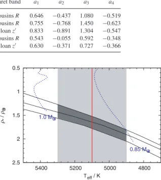
To choose the best model, we compared the discrete MM4 model, continuous MM2, MM3 and MM4 corresponding to fits with

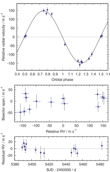
Bottom panel: Radial velocities from CORALIE (green) and HARPS (blue) with the adopted circular orbital model..

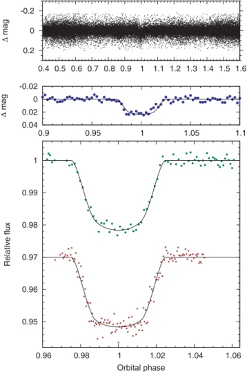
Fig. 2.—WASP-S, FTS, and EulerCam light curves showing the transit of WASP-4b. The data are shown folded on the orbital period together with the best-fitting model determined from

the apparent variability of the transit parameters deduced from the individual analysis of the light curves and their correlations, our interpretation of this increase of the <

The orbital parameters and the radius of the planet were estimated by best fitting the phase folded light curve with 34 successive transits.. Doppler measurements with the