HAL Id: hal-01661212
https://hal.archives-ouvertes.fr/hal-01661212
Submitted on 11 Dec 2017
HAL is a multi-disciplinary open access
archive for the deposit and dissemination of
sci-entific research documents, whether they are
pub-lished or not. The documents may come from
teaching and research institutions in France or
L’archive ouverte pluridisciplinaire HAL, est
destinée au dépôt et à la diffusion de documents
scientifiques de niveau recherche, publiés ou non,
émanant des établissements d’enseignement et de
recherche français ou étrangers, des laboratoires
Convolutional Neural Networks with Data
Augmentation against Jitter-Based Countermeasures.
Eleonora Cagli, Cécile Dumas, Emmanuel Prouff
To cite this version:
Eleonora Cagli, Cécile Dumas, Emmanuel Prouff. Convolutional Neural Networks with Data
Aug-mentation against Jitter-Based Countermeasures.. Cryptographic Hardware and Embedded Systems
- CHES 2017 - 19th International Conference, Sep 2017, Taipei, Taiwan. �hal-01661212�
Convolutional Neural Networks with Data
Augmentation against Jitter-Based
Countermeasures
– Profiling Attacks without Pre-Processing –
Eleonora Cagli1,2,4, C´ecile Dumas1,2, and Emmanuel Prouff3,4 1 Univ. Grenoble Alpes, F-38000, Grenoble, France 2
CEA, LETI, MINATEC Campus, F-38054 Grenoble, France {eleonora.cagli,cecile.dumas}@cea.fr
3
Safran Identity and Security, France [email protected]?? 4 Sorbonne Universit´es, UPMC Univ Paris 06, POLSYS, UMR 7606, LIP6, F-75005,
Paris, France
Abstract. In the context of the security evaluation of cryptographic implementations, profiling attacks (aka Template Attacks) play a fun-damental role. Nowadays the most popular Template Attack strategy consists in approximating the information leakages by Gaussian distri-butions. Nevertheless this approach suffers from the difficulty to deal with both the traces misalignment and the high dimensionality of the data. This forces the attacker to perform critical preprocessing phases, such as the selection of the points of interest and the realignment of measurements. Some software and hardware countermeasures have been conceived exactly to create such a misalignment. In this paper we pro-pose an end-to-end profiling attack strategy based on the Convolutional Neural Networks: this strategy greatly facilitates the attack roadmap, since it does not require a previous trace realignment nor a precise se-lection of points of interest. To significantly increase the performances of the CNN, we moreover propose to equip it with the data augmentation technique that is classical in other applications of Machine Learning. As a validation, we present several experiments against traces misaligned by different kinds of countermeasures, including the augmentation of the clock jitter effect in a secure hardware implementation over a mod-ern chip. The excellent results achieved in these experiments prove that Convolutional Neural Networks approach combined with data augmen-tation gives a very efficient alternative to the state-of-the-art profiling attacks.
Keywords: Side-Channel Attacks, Convolutional Neural Networks, Data Aug-mentation, Machine Learning, Jitter, Trace Misalignment, Unstable Clock ??
1
Introduction
To prevent Side-Channel Attacks (SCA), manufacturers commonly implement countermeasures that create misalignment in the measurements sets. The latter countermeasures are either implemented in hardware (unstable clock, random hardware interruption, clock stealing) or in software (insertion of random delays through dummy operations [8, 9], shuffling [33]). Until now two approaches have been developed to deal with misalignment problems. The first one simply consists in adapting the number of side-channel acquisitions (usually increasing it by a factor which is linear in the misalignment effect). Eventually an integration over a range of points [22] can be made, which guarantees the extraction of the information over a single point, at the cost of a linear increase of the noise, that may be compensated by the increase of the acquisitions. The second one, which is usually preferred, consists in applying realignment techniques in order to limit the desynchronization effects. Two realignment techniques families might be distinguished: a signal-processing oriented one (e.g. [25, 32]), more adapted to hardware countermeasures, and a probabilistic-oriented one (e.g. [11]), conceived for the detection of dummy operations, i.e. software countermeasures.
Among the SCAs, profiling attacks (aka Template Attacks, TA for short) play a fundamental role in the context of the security evaluation of crypto-graphic implementations. Indeed the profiling attack scenario allows to evaluate their worst-case security, admitting the attacker is able to characterize the device leakages by means of a full-knowledge access to a device identical to the one un-der attack. Such attacks work in two phases: first, a leakage model is estimated during a so-called profiling phase, then the profiled leakage model is exploited to extract key-dependent information in the proper attack phase. Approximating the information leakage by a Gaussian distribution is today the most popular approach for the profiling, due to its theoretical optimality when the noise tends towards infinity. Nevertheless the performances of such a classical TA highly depend on some preliminary phases, such as the traces realignment or the se-lection of the Points of Interest (PoIs). Indeed the efficiency/effectiveness of the Gaussian approximation is strongly impacted by the dimension of the leakage traces at input.
In this paper we propose the use of a Convolutional Neural Network (CNN) as a comprehensive profiling attack strategy. Such a strategy, divided into a learning phase and a proper attack phase, can replace the entire roadmap of the state of the art attacks: for instance, contrary to a classical TA, any trace prepro-cessing such as realignment or the choice of the PoIs are included in the learning phase. Indeed we will show that the CNNs implicitly perform an appropriate combination of the time samples and are robust to trace misalignment. This property makes the profiling attacks with CNNs efficient and easy to perform, since they do not require critical preprocessings. Moreover, since the CNNs are less impacted than the classical TA by the dimension of the traces, we can a pri-ori expect that their efficiency outperforms (or at least perform as well as) the classical TAs. Indeed, CNNs can extract information from a large range of points while, in practice, Gaussian TAs are used to extract information on some
pre-viously dimensionality-reduced data (and dimensionality reduction never raises the informativeness of the data [10]). This claim, and more generally the sound-ness and the efficiency of our approach, will be proven by several experiments throughout this paper.
To compensate some undesired behaviour of the CNNs, we propose as well to embed them with Data Augmentation (DA) techniques [30, 34], recommended in the machine learning domain for improving performances: the latter tech-nique consists in artificially generating traces in order to increase the size of the profiling set. To do so, the acquired traces are distorted through plausible transformations that preserve the label information (i.e. the value of the han-dled sensitive variable in our context). Actually, in this paper we propose to turn the misalignment problem into a virtue, enlarging the profiling trace set via a random shift of the acquired traces and another typology of distortion that to-gether simulate a clock jitter effect. Paradoxically, instead of trying to realign the traces, we propose to further misalign them (a much easier task!), and we show that such a practice provides a great benefit to the CNN attack strategy.
This contribution makes part of the transfer of methodology in progress in last years from the machine learning and pattern recognition domain to the side-channel analysis one. Recently the strict analogy between template attacks and the supervised classification problem as been depicted [16], while the deployment of Neural Networks (NNs) [24, 23, 35] and CNNs [21] to perform profiled SCAs has been proposed. Our paper aims to pursue this line of works.
This paper focuses over the robustness of CNNs to misalignment, thus consid-erations about other kinds of countermeasures, such as masking, are left apart. Nevertheless, the fact that CNNs usually applies non-linear functions to the data makes them potentially (and practically, as already experienced in [21]) able to deal with such a countermeasure as well.
The paper is organized as follows: in Sec. 2 we recall the classical TA roadmap, we introduce the MLP family of NNs, we describe the NN-based SCA and we finally discuss the practical aspects of the training phase of an NN. In Sec. 3 the basic concepts of the CNNs are introduced, together with the description of the deforming functions we propose for the data augmentation. In Sec. 4 we test the CNNs against some software countermeasures, in order to validate our claim of robustness to the misalignment caused by shifting. Experiments against hardware countermeasures are described in Sec. 5, proving that the CNN are robust to deformations due to the jitter.
2
Preliminaries
2.1 Notations
Throughout this paper we use calligraphic letters as X to denote sets, the corre-sponding upper-case letter X to denote random variables (random vectors if in bold X) over X , and the corresponding lower-case letter x (resp. x for vectors) to denote realizations of X (resp. X). The i-th entry of a vector x is denoted
by x[i]. The symbol E denotes the expected value, and might be subscripted by a random variable EX, or by a probability distribution Ep(X), to specify un-der which probability distribution it is computed. Side-channel traces will be viewed as realizations of a random column vector X ∈ RD. During their ac-quisition, a target sensitive variable Z = f (P, K) is handled, where P denotes some public variable, e.g. a plaintext, and K the part of secret key the attacker aims to retrieve. The value assumed by such a variable is viewed as a realiza-tion z ∈ Z = {z1, z2, . . . , z|Z|} of a discrete finite random variable Z. We will sometimes represent the values zj ∈ Z via the so-called one-hot encoding rep-resentation, assigning to zj a |Z|-dimensional vector, with all entries equal to 0 and the j-th entry equal to 1: zj → zj = (0, . . . , 0, 1
|{z} j
, 0, . . . , 0). Under this notation, the random variable Z turns into a random vector Z.
2.2 Profiling Side-Channel Attack
A profiling SCA is composed of two phases: a profiling (or characterization, or training) phase, and an attack (or matching) phase. During the first one, the attacker estimates the probability:
Pr[X|Z = z] , (1)
from a profiling set {xi, zi}i=1,...,Npof size Np, which is a set of traces xiacquired under known value zi of the target. The potentially huge dimensionality of X lets such an estimation a very complex problem, and the most popular way adopted until now to estimate the conditional probability is the one that led to the well-established Gaussian TA [5] (aka Quadratic Discriminant Analysis [12]). To perform the latter attack, the adversary priorly exploits some statistical tests (e.g. SNR or T-Test) and/or dimensionality reduction techniques (e.g. Principal Component Analysis, Linear Discriminant Analysis [12], Kernel Discriminant Analysis [4]) to select a small portion of PoIs or an opportune combination of them. Then, denoting ε(X) the result of such a dimensionality reduction, the attacker assumes that ε(X)|Z has a multivariate Gaussian distribution, and estimates the mean vector µz and the covariance matrix Σz for each z ∈ Z (i.e. the so-called templates). In this way the pdf (1) is approximated by the Gaussian pdf with parameters µz and Σz. The attack phase eventually consists in computing the likelihood of the attack set {xi}i=1,...,N for each template and in sorting the key candidates k ∈ K with respect to their score dk defined such that: dk = N Y i=1 Pr[Z = f (pi, k)|ε(X) = ε(xi)] = N Y i=1 Pr[ε(X) = ε(xi)|Z = f (pi, k)] Pr[Z = f (pi, k))] , (2) where (2) is obtained via Bayes’ Theorem under the hypothesis that acquisitions are independent.1
1
In TA the profiling set and the attack set are assumed to be different, namely the traces xiinvolved in (2) have not been used for the profiling.
Traces misalignment affects the approach above. In particular, if not treated with a proper realignment, it makes the PoI selection harder, obliging the at-tacker to consider a wide range of points for the characterization and matching (the more effective the misalignment, the wider the range), directly or after a previous integration [7] or a dimension reduction methods.2As we will see in the next section, neural networks, and in particular the CNNs, are able to efficiently and simultaneously address the PoI selection problem and the misalignment issue. More precisely, they can be trained to search for informative weighted combinations of leakage points, in a way that is robust to traces misalignment.
2.3 Neural Networks and the Multi-Layer Perceptron
The classification problem is the most widely studied one in machine learning, since it is the central building block for all other problems, e.g detection, regres-sion, etc. [3] It consists in taking an input, e.g. a side-channel trace x, and in assigning it a label z ∈ Z, e.g. the value of the target variable handled during the acquisition. In the typical setting of a supervised classification problem, a training set is available, which is a set of data already assigned to the right label. The latter set exactly corresponds to the profiling set in the side-channel context.
Neural networks (NN) are nowadays the privileged tool to address the clas-sification problem. They aim at constructing a function F : RD
→ R|Z| that takes data x ∈ RD
and outputs vectors y ∈ R of scores. The classification of x is done afterwards by choosing the label zj such that j = argmax y[j]. In general F is obtained by combining several simpler functions, called layers. An NN has an input layer (the identity over the input datum x), an output layer (the last function, whose output is the scores vector y) and all other layers are called hidden layers. The nature (the number and the dimension) of the layers is called the architecture of the NN. All the parameters that define an architecture, together with some other parameters that govern the training phase, have to be carefully set by the attacker, and are called hyper-parameters. The so-called neu-rons, that give the name to the NNs, are the computational units of the network and essentially process a scalar product between the coordinates of its input and a vector of trainable weights (or simply weights) that have to be trained. Each layer processes some neurons and the outputs of the neuron evaluations will form new input vectors for the subsequent layer. The training phase consists in an automatic tuning of the weights and it is done via an iterative approach which locally applies the Stochastic Gradient Descent algorithm [13] to minimize a loss function quantifying the classification error of the function F over the training set. We will not give further details about this classical optimization approach, and the interested reader may refer to [13].
In this paper we focus on the family of the Multi-Layer Perceptrons (MLPs). They are associated with a function F that is composed of multiple linear
func-2
tions and some non-linear activation functions which are efficiently-computable and whose derivatives are bounded and efficient to evaluate. To sum-up, we can express an MLP by the following equation:
F (x) = s ◦ λn◦ σn−1◦ λn−1◦ · · · ◦ λ1(x) = y , (3) where:
– the λi functions are the so-called Fully-Connected (FC) layers and are ex-pressible as affine functions: denoting x ∈ RDthe input of an FC, its output is given by Ax + b, being A ∈ RD×C
a matrix of weights and b ∈ RC a vector of biases. These weights and biases are the trainable weights of the FC layer.3
– the σi are the so-called activation functions (ACT): an activation function is a non-linear real function that is applied independently to each coordinate of its input,
– s is the so-called softmax4function (SOFT): s(x)[i] = ex[i] P
jex[j] .
Examples of ACT layers are the sigmoid f (x)[i] = (1 + e−x[i])−1 or the rec-tified linear unit (ReLU) f (x)[i] = max(0, x[i]). In general they do not depend on trainable weights.
The role of the softmax is to renormalise the output scores in such a way that they define a probability distribution y ≈ Pr[Z|X = x].
In this way, the computed output does not only provide the most likely label to solve the classification problem, but also the likelihood of the remaining |Z|−1 other labels. In the profiling SCA context, this form of output allows us to enter it in (2) (setting the preprocessing function ε equal to the identity) to rank key candidates; actually (3) may be viewed as an approximation of the pdf in (1).5 We can thus rewrite (2) as:
dk= N Y
i=1
F (xi)[f (pi, k)]. (4)
We refer to [20] for an (excellent) explication over the relationship between the softmax function and the Bayes theorem.
3
They are called Fully-Connected because each i-th input coordinate is connected to each j-th output via the A[i, j] weight. FC layers can be seen as a special case of the linear layers in general Feed-Forward networks, in which not all the connections are present. The absence of some (i, j)-th connections can be formalized as a constraint for the matrix A consisting in forcing to 0 its (i, j)-th coordinates.
4
To prevent underflow, the log-softmax is usually preferred if several classification outputs must be combined.
5
Remarkably, this places SCAs based on MLP as a particular case of the classical profiling attack that exploits the maximum likelihood as distinguisher.
2.4 Practical Aspects of the Training Phase and Overfitting
The goal of the training phase is to tune the weights of the NN. The latter ones are first initialized with random values and are afterwards updated by applying several times the same process: a batch of traces (xi)i∈Ichosen in random order (here I is a random set of indexes) goes through the network to process the corresponding scores (yi = F (xi))i∈I, the loss function is evaluated from these scores and finally the loss is reduced by modifying the trainable parameters, subtracting from them a small multiple of the loss gradient. Fro our experiments and simulations, we selected the the averaged cross-entropy between each yi and the corresponding correct label zias loss function. Indeed nowadays this is the recommended choice for classification problems [13]. There are two ways to interpret such a choice.
– First, recalling that yimay be interpreted as an estimation of the conditional probability Pr[Z|X = xi], the principle of maximum-likelihood suggests to drive the training in such a way that for such an estimate the probability of the correct label zi is as high as possible. Thus, if we suppose the correct label vector zi= (0, . . . , 0, 1
|{z} j
, 0, . . . , 0) corresponds to the one-hot encoding of the label zj, we want to maximize y
i[j] (or equivalently to minimize − log yi[j]).6It may be observed that such a log-likelihood rewrites as
− log yi[j] = − |Z| X
t=1
zi[t] log yi[t] . (5)
– The second interpretation of the choice of the average cross-entropy comes from the observation that the vector zi = (0, . . . , 0, 1
|{z} j
, 0, . . . , 0) gives the value of the pmf of Z|Z = zi, which corresponds to the exact probabil-ity densprobabil-ity we want the network to approximate. Informally speaking, the cross-entropy between two probability distributions zi, yigives a measure of dissimilarity between them, and is defined as follows:
H(zi, yi) = H(zi) + DKL(zi||yi) = Ezi[− log yi] = − |Z| X
t=1
zi[t] log yi[t] , (6)
where H denotes the entropy and DKL denotes the Kullback-Leibler diver-gence (see [3]-Sec. 1.6). Thus, this is an information-theoretic notion, that comes out to be equivalent to the negative log-likelihood formula given by (5).
In conclusion, depending on the point of view, minimizing the cross-entropy corresponds to maximize the likelihood of the right label, or to minimize the
6
We remark that thanks to the softmax function used as last network layer, each coordinate of yi is always strictly positive.
dissimilarity between the network estimation of a distribution and the right distribution that we want it to approximate. In practice, to train the neural network the loss function is given by the cross-entropy averaged over the traces contained in a batch: L(F, (xi)i∈I) = 1 | I | X i∈I H(zi, F (xi)) . (7)
A good choice for the size of the batch is a value as large as possible but which avoids computational performances drop. An iteration over the entire training set is called epoch. To monitor the training of an NN and to evaluate its performances it is a good practice to separate the labelled data into 3 sets:
– the proper training set, which is actually used to train the weights (in general it contains the greatest part of the labelled data)
– a validation set, which is observed in general at the end of each epoch to monitor the training
– a test set, which is kept unobserved during the training phase and which is involved to finally evaluate the performances of the trained NN.
For our experiments we will use the attack traces as test set, while we will split the profiling traces into a training set and a validation set.7
The accuracy is the most common metric to both monitor and evaluate an NN. It is defined as the successful classification rate reached over a dataset. The training accuracy, the validation accuracy and the test accuracy are the success-ful classification rates achieved respectively over the training, the validation and the test sets. At the end of each epoch it is useful to compute and to compare the training accuracy and the validation accuracy. For some trained models we will measure in this paper (see e.g. Table 1) the following two additional quantities: – the maximal training accuracy, corresponding to the maximum of the
train-ing accuracies computed at the end of each epoch
– the maximal validation accuracy, corresponding to the maximum of the val-idation accuracies computed at the end of each epoch.
In addition to the two quantities above, we will also evaluate the performances of our trained model, by computing a test accuracy. Sometimes it is useful to complete this evaluation by looking at the so-called confusion matrix (see the
7
The way how the profiling set is split into training and validation sets might induce a bias in the learned model. A good way to get rid of such a bias is to apply a cross-validation technique, e.g. a 10-fold cross-validation. The latter one consists in partitioning the profiling set into 10 sub-sets, and in performing 10 times the training while choosing each time one of the sub-sets for the validation and the union of the 9 other ones for the training. An average over the performances of the 10 obtained models gives a more robust estimation of the accuracies and performances. Results of this papers do not make use of such a cross-validation technique.
bottom part of Fig. 5). Indeed the latter matrix enables, in case of misclassi-fication, for the identification of the classes which are confused. The confusion matrix corresponds to the distribution over the couples (true label, predicted la-bel) directly deduced from the results of the classification on the test set. A test accuracy of 100% corresponds to a diagonal confusion matrix.
On the Need to also Consider the Guessing Entropy. The accuracy metric is perfectly adapted to the machine learning classification problem, but corresponds in side-channel language to the success rate of a Simple Attack, i.e. an attack where a single attack trace is available. When the attacker can acquire several traces for varying plaintexts, the accuracy metric is not sufficient alone to evaluate the attack performance. Indeed such a metric only takes into account the label corresponding to the maximal score and does not consider the other ones, whereas an SCA through (4) does (and therefore exploits the full information).
To take this remark into account, we will always associate the test accuracy to a side-channel metric defined as the minimal number N?of side-channel traces that makes the guessing entropy (the average rank of the right key candidate) be permanently equal to 1 (see e.g. Table 1). We will estimate such a guessing entropy through 10 independent attacks.
As we will see in the sections dedicated to our attack experiments, applying Machine Learning in a context where at the same time (1) the model to recover is complex and (2) the amount of exploitable measurements for the training is limited, may be ineffective due to some overfitting phenomena.
Overfitting. Often the training accuracy is higher than the validation one. When the gap between the two accuracies is excessive, we assist to the overfit-ting phenomenon. It means that the NN is using its weights to learn by heart the training set instead of detecting significant discriminative features. For this reason its performances are poor over the validation set, which is new to it. Over-fitting occurs when an NN is excessively complex, i.e. when it is able to express an excessively large family of functions. In order to keep the NN as complex as wished and hence limiting the overfitting, some regularization techniques can be applied. For example, in this paper we will propose the use of the Data Augmen-tation (DA) [30] that consists in artificially adding observations to the training set. Moreover we will take advantage of the early-stopping technique [27] that consists in well choosing a stop condition based on the validation accuracy or on the validation loss (i.e. the value taken by the loss function over the validation set).
3
Convolutional Neural Networks
In this section we describe the layers that turn an MLP into a Convolutional Neural Network (CNN), and we explain how the form of these layers makes the CNNs robust to misalignment. Then we will specify the Data Augmentation that can be applied in our context, in order to deal with overfitting.
3.1 Description of the CNNs
The CNNs complete the classical principle of MLP with two additional types of layers: the so-called convolutional layer based on a convolutional filtering, and a pooling layer. We describe these two particular layers hereafter.
Convolutional (CONV) layers are linear layers that share weights across space. The representation is given in Fig. 1-(a).8 To apply a convolutional layer to an input trace, V small column vectors, called convolutional filter, of size W are slid over the trace.9 The column vectors form a window which defines a linear transformation of W consecutive points of the trace into a new vector of V points. The coordinates of the window (viewed as a matrix) are among the trainable weights and are constrained to be unchanged for every input window. This constraint is the main difference between a CONV layer and an FC layer; it allows the former to learn shift-invariant features. The reason why several filters are applied is that we expect each filter to extract a different kind of char-acteristic from the input. As one goes along convolutional layers, higher-level abstraction features are expected to be extracted. These high-level features are arranged side-by-side over an additional data dimension, the so-called depth.10 This is this geometric characteristic that makes CNNs robust to temporal defor-mations [19].
To avoid complexity explosion due to this depth increasing, the insertion of pooling layers is recommended.
Pooling (POOL) layers are non-linear layers that reduce the spatial size in order to limit the amount of neurons, and by consequence the complexity of the minimization problem (see Fig. 1-(b)). As the CONV layers, they make some filters slide across the input. Filters are 1-dimensional, characterised by a length W , and usually the stride5is chosen equal to their length; for example in Fig.1(b) both the length and the stride equal 3, so that the selected segments of the input 8 CNNs have been introduced for images [19]. So, usually, layer interfaces are arranged in a 3D-fashion (height, weight and depth). In Fig. 1(a) we show a 2D-CNN (length and depth) adapted to 1D-data as side-channel traces are.
9
The amount of units by which the filter shifts across the trace is called stride. In Fig. 1-(a) the stride equals 1.
10
Ambiguity: NNs with many layers are sometimes called Deep Neural Networks, where the depth corresponds to the number of layers.
2 3 1 1 -1 8 1 9 0 4 1 2 1 0 -1 8 5 4 5 3 Input Trace Le n gth = 9 Depth = 1 Depth = 4 Filtered Trace 4 convolutional filters of size 2 2 5 8 15 1 (a) 2 9 1 7 2 5 1 4 8 4 1 10 3 4 1 1 5 15 7 2 4 4 2 9 3 3 1 9 5 3 4 5 2 Le n gth = 9 Depth = 4 After Pooling 10 4 15 7 9 3 9 5 9 7 8 8 Before Pooling Depth = 4 Max Pooling Filter Length = 3 Stride = 3 8 5 5 (b)
Fig. 1: (a) Convolutional filtering: W = 2, V = 4, stride = 1. (b) Max-pooling layer: W = stride = 3.
do not overlap. In contrast with convolutional layers, the pooling filters do not contain trainable weights. They only slide across the input to select a segment, then a pooling function is applied: the most common pooling functions are the max-pooling which outputs the maximum values within the segment and the average-pooling which outputs the average of the coordinates of the segment. Common architecture The main block of a CNN is a CONV layer γ directly followed by an ACT layer σ. The former locally extracts information from the input thanks to filters and the latter increases the complexity of the learned classification function thanks to its non-linearity. After some (σ ◦ γ) blocks, a POOL layer δ is usually added to reduce the number of neurons: δ ◦ [σ ◦ γ]n2. This new block is repeated in the neural network until obtaining an output of reasonable size. Then, some FC are introduced in order to obtain a global result which depends on the entire input. To sum-up, a common convolutional network can be characterized by the following formula:11
s ◦ [λ]n1◦ [δ ◦ [σ ◦ γ]n2]n3. (8) Layer by layer it increases depth through convolution filters, adds non-linearity through activation functions and reduces spatial (or temporal, in the side-channel traces case) size through pooling layers. Once a deep and narrow representation has been obtained, one or more FC layers are connected to it, followed by a softmax function. An example of CNN architecture is represented in Fig. 2.
3.2 Data Augmentation
As pointed out in Sec.2.4, it is sometimes necessary to manage the overfitting phenomenon, by applying some regularization techniques. As we will see in Secs. 11where each layer of the same type appearing in the composition is not to be intended as exactly the same function (e.g. with same input/output dimensions), but as a function of the same form.
Sid e -Chan n e l T race Convolution + Activation + Pooling Convolution + Activation + Pooling Convolution + Activation + Pooling
Fully Connected Layer + Softmax
Temporal Features
Abstract Features Scores
Fig. 2: Common CNN architecture
4 and 5 this will be the case in our experiments: indeed we will propose a quite deep CNN architecture, flexible enough to manage the misalignment problems, but trained over some relatively small training sets. This fact, combined with the high number of weights exploited by our CNN implies that the latter one will learn by heart each element of the training set, without catching the truly discriminant features of the traces.
Among all regularization techniques, we choose to concentrate priorly on the Data Augmentation [30], mainly for two reasons. First, it is well known that the presence of misalignment forces to increase the number of acquisitions. In other terms, misalignment may provoke a lack of data phenomenon on the ad-versary side. In the machine learning domain such a lack is classically addressed thanks to the DA technique, and its benefits are widely proved. For example, many image recognition competition winners made use of such a technique (e.g. the winner of ILSVRC-2012 [18]). Second, the DA is controllable, meaning that the deformations applied to the data are chosen, thus fully characterized. It is therefore possible to fully determine the addition of complexity induced to the classification problem. In our opinion, other techniques add constraints to the problem in a more implicit way, e.g. the dropout [15] or the `2-norm regulariza-tion [3].
Data augmentation consists in artificially generating new training traces by deforming those previously acquired. The deformation is done by the application of transformations that preserve the label information (i.e. the value of the handled sensitive variable in our context). We choose two kinds of deformations, that we denote by Shifting and Add-Remove.
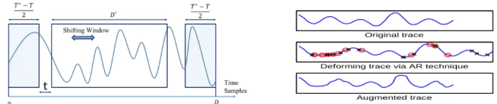
Shifting Deformation (SHT?) simulates a random delay effect of maximal am-plitude T?, by randomly selecting a shifting window of the acquired trace, as shown in Fig. 3. Let D denote the original size of the traces. We fix the size of
𝑇∗− 𝑇 2 𝑇∗− 𝑇 2 0 t 𝐷′ 𝐷 Shifting Window Time Samples Original trace
Deforming trace via AR technique
Augmented trace
Fig. 3: Left: Shifting technique for DA. Right: Add-Remove technique for DA (added points marked by red circles, removed points marked by black crosses).
the input layer of our CNN to D0= D − T?. Then the technique SHT? consists (1) in drawing a uniform random t ∈ [0, T?], and (2) in selecting the D0-sized window starting from the t-th point. For our study, we will compare the SHT technique for different values T ≤ T?, without changing the architecture of the CNN (in particular the input size D0). Notably, T T? implies that T?− T time samples will never have the chance to be selected. As we suppose that the information is localized in the central part of the traces, we choose to center the shifting windows, discarding the heads and the tails of the traces (corresponding to the first and the last T?2−T points).
Add-Remove Deformation (AR) simulates a clock jitter effect (Fig. 3). We will denote by ARRthe operation that consists (1) in inserting R time samples, whose positions are chosen uniformly at random and whose values are the arithmetic mean between the previous time sample and the following one, (2) in suppressing R time samples, chosen uniformly at random.
The two deformations can be composed: we will denote by SHTARR the application of a SHT followed by a ARR.
4
Application to software countermeasures
In this section we present a preliminary experiment we have performed in order to validate the shift-invariance claimed by the CNN architecture, recalled in Sec. 3.1. In this experiment a single leaking operation was observed through the side-channel acquisitions, shifted in time by the insertion of a random number of dummy operations. A CNN-based attack is run, successfully, without effectuating any priorly realignment of the traces. We also performed a second experiment in which we targeted two leaking operations.
We believe (and we discuss it in more details in Appendix B) that dealing with dummy operations insertion does not represent an actual obstacle for an attacker nowadays. Thus, the experiment we present in this section is not expected to be representative of real application cases. Actually, we think that the CNNs bring a truly great advantage with respect to the state-of-the-art TAs in presence of hardware-flavoured countermeasures, such as augmented jitter effects. We refer to Sec. 5 for experiments in such a context.
0 1000 2000 3000 4000 −0.5 0 0.5 0 1000 2000 3000 4000 −0.5 0 0.5 0 1000 2000 3000 4000 −0.5 0 0.5 Time samples Power Consumption 0 1000 2000 3000 4000 −0.5 0 0.5 0 1000 2000 3000 4000 −0.5 0 0.5 0 1000 2000 3000 4000 −0.5 0 0.5 Time samples Power consumption
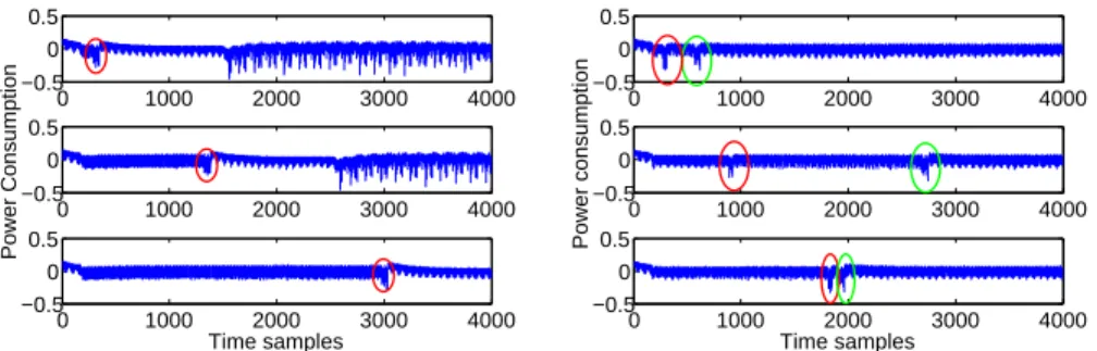
Fig. 4: Left: one leakage protected by single uniform RDI. Right: two leaking operations protected by multiple uniform RDI.
CNN-based Attack against Random Delays. For this experiment, we im-plemented, on an Atmega328P microprocessor, a uniform Random Delay Inter-rupt (RDI) [31] to protect the leakage produced by a single target operation. Our RDI simply consists in a loop of r nop instructions, with r drawn uniformly in [0, 127].
Some acquired traces are reported in the left side of Fig. 4, the target peak being highlighted with a red ellipse. They are composed of 3, 996 time samples, corresponding to an access to the AES-Sbox look-up table stored in NVM. For the training, we acquired only 1, 000 traces and 700 further traces were acquired as validation data. Our CNN has been trained to classify the traces according to the Hamming weight of the Sbox output; namely, our labels are the 9 values taken by Z = HW(Sbox(P ⊕ K)). This choice has been done to let each class contain more than only a few (i.e. about 1, 000/256) training traces.12Since Z is assumed to take 9 values and the position of the leakage depends on a random r ranging over 128 values, it is clear that the 1, 000 training traces do not encompass the full 9 × 128 = 1, 152 possible combinations (z, r) ∈ [0, 8] × [0, 127]. We undersized the training set by purpose, in order to establish whether the CNN technique, equipped with DA, is able to catch the meaningful shift-invariant features without having been provided with all the possible observations.
For the training of our CNN, we applied the SHT data augmentation, se-lecting T?= 500 and T ∈ {0, 100, T?}; this implies that the input dimension of our CNN is reduced to 3, 496. Our implementation is based on Keras library [1] (version 1.2.1), and we run the trainings over an ordinary computer equipped with a gamers market GPU, as specified in Sec. 5.2. For the CNN architecture, we chose the following architecture:
s ◦ [λ]1◦ [δ ◦ [σ ◦ γ]1]4, (9) i.e. (8) with n1= n2= 1 and n3 = 4. To accelerate the training we introduced a Batch Normalization layer [17] after each pooling δ. The network transforms 12
For Atmega328P devices, the Hamming weight is known to be particularly relevant to model the leakage occurring during register writing [2].
0 20 40 60 80 100 120 Epoch 0.2 0.3 0.4 0.5 0.6 0.7 0.8 0.9 1.0 training accuracy validation accuracy 0 20 40 60 80 100 120 140 Epoch 0.2 0.3 0.4 0.5 0.6 0.7 0.8 0.9 1.0 training accuracy validation accuracy 0 50 100 150 200 250 300 Epoch 0.2 0.4 0.6 0.8 training accuracy validation accuracy 0 1 2 3 4 5 6 7 8Predicted label 0 1 2 3 4 5 6 7 8 True label 0 0 0 2 3 0 0 0 0 0 0 0 4 20 0 0 0 0 0 0 0 24 75 0 0 0 0 0 0 0 671630 0 0 0 0 0 0 892030 0 0 0 0 0 0 721460 0 0 0 0 0 0 25 70 0 0 0 0 0 0 0 11 22 0 0 0 0 0 0 0 0 4 0 0 0 0 0 25 50 75 100 125 150 175 200 0 1 2 3 4 5 6 7 8 Predicted label 0 1 2 3 4 5 6 7 8 True label 0 0 2 2 1 0 0 0 0 0 1 4 10 7 1 1 0 0 0 1 1858 14 8 0 0 0 0 0 2611452 36 2 0 0 0 0 1497 76 99 6 0 0 0 0 3 44 60 1029 0 0 0 0 1 7 26 54 7 0 0 0 0 0 1 6 22 4 0 0 0 0 0 0 1 3 0 0 0 0 15 30 45 60 75 90 105 0 1 2 3 4 5 6 7 8 Predicted label 0 1 2 3 4 5 6 7 8 True label 0 4 0 0 1 0 0 0 0 0 15 4 2 1 1 1 0 0 0 2 80 14 2 1 0 0 0 0 0 1520014 0 1 0 0 0 0 1 3422928 0 0 0 0 2 0 1 2717414 0 0 0 0 0 0 4 18 65 8 0 0 0 0 0 1 2 13 17 0 0 0 0 0 0 0 1 3 0 0 25 50 75 100 125 150 175 200 225
Fig. 5: One leakage protected via single uniform RDI: accuracies vs epochs and confu-sion matrices obtained with our CNN for different DA techniques. From left to right: SH0, SH100, SH500.
Table 1: Results of our CNN, for different DA techniques, in presence of an uniform RDI countermeasure protecting. For each technique, 4 values are given: in position a the maximal training accuracy, in position b the maximal validation accuracy, in position c the test accuracy, in position d the value of N?(see Sec. 2.4 for definitions).
SH0 SH100 SH500
a b 100% 25.9% 100% 39.4% 98.4% 76.7%
c d 27.0% >1000 31.8% 101 78.0% 7
the 3, 496 × 1 inputs in a 1 × 256 list of abstract features, before entering the last FC layer λ : R256→ R9. Even if the ReLU activation function [26] is classically recommended for many applications in literature, we obtained in most cases bet-ter results using the hyperbolic tangent. We trained our CNN by batches of size 32. In total the network contained 869, 341 trainable weights. The training and validation accuracies achieved after each epoch are depicted in Fig.5 together with the confusion matrices that we obtained from the test set. Applying the early-stopping principle recalled in Sec. 2.4, we automatically stopped the train-ing after 120 epochs without decrement of the loss function evaluated over the validation set, and kept as final trained model the one that showed the minimal value for the loss function evaluation. Concerning the learning rate, i.e. the fac-tor defining the size of the steps in the gradient descent optimization (see [13]), we fixed the beginning one to 0.01 and reduced it multiplying it by a factor of √
0.1 after 5 epochs without validation loss decrement.
Table 1 summarizes the obtained results. For each trained model we can com-pare the maximal training accuracy achieved during the training with the maxi-mal validation accuracy (see Sec. 2.4 for the definition of these accuracies). This
comparison gives an insight about the risk of overfitting for the training.13Case SH0 corresponds to a training performed without DA technique. When no DA is applied, the overfitting effect is dramatic: the training set is 100%-successfully classified after about 22 epochs, while the test accuracy only achieves 27%. The 27% is around the rate of uniformly distributed bytes showing an Hamming weight of 4.14 Looking at the corresponding confusion matrix we remark that the CNN training has been biased by the binomial distribution of the training data, and almost always predicts the class 4. This essentially means that no dis-criminative feature has been learned in this case, which is confirmed by the fact that the trained model leads to an unsuccessful attack (N? > 1, 000). Remark-ably, the more artificial shifting is added by the DA, the more the overfitting effect is attenuated; for SHT with e.g. T = 500 the training set is never com-pletely learnt and the test accuracy achieves 78%, leading to a guessing entropy of 1 with only N?= 7 traces.
These results confirm that our CNN model is able to characterize a wide range of points in a way that is robust to RDI.
Two leaking operations. In this section we study whether our CNN classifier suffers from the presence of multiple leaking operations with the same power consumption pattern. This situation occurs for instance any time the same op-eration is repeated several successive times over different pieces of data (e.g. the SubByte operation for a software AES implementation is often performed by 16 successive look-up table access). To start our study we performed the same ex-periments as in Sec. 4 over a second traces set, where two look-up table accesses leak, each preceded by a random delay. Some examples of this second traces set are given in the right side of Fig. 4, where the two leaking operations being highlighted by red and green ellipses. We trained the same CNN as in Sec. 4, once to classify the first leakage, and a second time to classify the second leak-age, applying SH500. Results are given in Table 2. They show that even if the CNN transforms spatial (or temporal) information into abstract discriminative features, it still holds an ordering notion: indeed if no ordering notion would have been held, the CNN could no way discriminate the first peak from the second one.
5
Application to hardware countermeasures
A classical hardware countermeasure against side-channel attacks consists in in-troducing instability in the clock. This implies the cumulation of a deforming 13
The validation accuracies are estimated over a 700-sized set, while the test accuracies are estimated over 100, 000 traces. Thus the latter estimation is more accurate, and we recall that the test accuracy is to be considered as the final CNN classification performance.
14
We recall that the Hamming weight of uniformly distributed data follows a binomial law with coefficients (8, 0.5).
Table 2: Results of our CNN in presence of uniform RDI protecting two leaking operations. See the caption Table 1 for a legend.
First operation Second operation
a b 95.2% 79.7% 96.8% 81.0%
c d 76.8% 7 82.5% 6
effect that affects each single acquired clock cycle, and provokes traces misalign-ment on the adversary side. Indeed, since clock cycles do not have the same duration, they are sampled during the attack by a varying number of time sam-ples. As a consequence, a simple translation of the acquisitions is not sufficient in this case to align w.r.t. an identified clock cycle. Several realignment tech-niques are available to manage this kind of deformations, e.g. [32]. The goal of this paper is not to compare a new realignment technique with the existing ones, but to show that we can get rid of the realignment pre-processing exploiting the end-to-end attack strategy provided by the CNN approach.
5.1 Performances over Artificial Augmented Clock Jitter
In this section we present the results that we obtained over two datasets named DS low jitter and DS high jitter. Each one contains 10, 000 labelled traces, used for the training/profiling phase (more precisely, 9, 000 are used for the training, and 1, 000 for the validation), and 100, 000 attack traces. The traces are com-posed of 1, 860 time samples. The two datasets have been obtained by artificially adding a simulated jitter effect over some synchronized original traces. The orig-inal traces were measured on the same Atmega328P microprocessor used in the previous section. We verified that they originally encompass leakage on 34 in-structions: 2 nops, 16 loads from the NVM and 16 accesses to look-up tables. For our attack experiments, it is assumed that the target is the first look-up table access, i.e. the 19th clock cycle. As in the previous section, the target is assumed to take the form Z = HW(Sbox(P ⊕ K)). To simulate the jitter ef-fect each clock pattern has been deformed15 by adding r new points if r > 0 (resp. removing r points if r < 0), with r ∼ N (0, σ2).16 For the DS low jitter dataset, we fixed σ2 = 4 and for the DS high jitter dataset we fixed σ2 = 36. As an example, some traces of DS low jitter are depicted in the left-hand side of Fig. 6: the cumulative effect of the jitter is observable by remarking that the desynchronization raises with time. Some traces of DS high jitter are depicted as well in the right-hand side of Fig. 6. For both datasets we did not operate any PoI selection, but entered the entire traces into our CNN.
We used the same CNN architecture (9) as in previous section. We assisted again to a strong overfitting phenomenon and we successfully reduced it by applying the DA strategy introduced in Sec. 3.2. This time we applied both the shifting deformation SHT with T?= 200 and T ∈ {0, 20, 40} and the add-remove 15
The 19th clock cycle suffers from the cumulation of the previous 18 deformations 16
Fig. 6: Left: some traces of the DS low jitter dataset, a zoom of the part highlighted by the red rectangle is given in the bottom part. Right: some traces (and the relative) of the DS high jitter dataset. The interesting clock cycle is highlighted by the grey rectangular area.
deformation ARR with R ∈ {0, 100, 200}, training the CNN model using the 9 combinations SHTARR. We performed a further experiment with much higher DA parameters, i.e. SH200AR500, to show that the benefits provided by the DA are limited: as expected, too much deformation affects the CNN performances (indeed results obtained with SH200AR500 will be worse than those obtained with e.g. SH40AR200). 100 101 102 103 104 0 50 100 150 200
Number of attack traces
Guessing Entropy
Gaussian TA wo realignment Gaussian TA with realignment Our CNN − SH 40 − AR200 100 101 102 103 104 0 50 100 150
Number of attack traces
Guessing Entropy
Gaussian TA wo realignment Gaussian TA with realignment Our CNN − SH
20 − AR200
Fig. 7: Comparison between a Gaussian template attack, with and without realign-ment, and our CNN strategy, over the DS low jitter (left) and the DS high jitter (right).
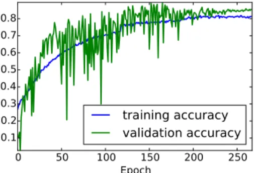
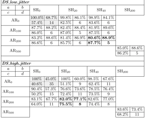
The results we obtained are summarized in Table 3. Case SH0AR0 corre-sponds to a training performed without DA technique (and hence serves as a reference suffering from the overfitting phenomenon). It can be observed that as the DA parameters raise, the validation accuracy increases while the train-ing accuracy decreases. This experimentally validates that the DA technique is efficient in reducing overfitting. Remarkably in some cases, for example in the DS low jitter dataset case with SH100AR40, the best validation accuracy is higher than the best training accuracy. In Fig. 8 the training and validation ac-curacies achieved in this case epoch by epoch are depicted. It can be noticed that
the unusual relation between the training and the validation accuracies does not only concern the maximal values, but is almost kept epoch by epoch. Observing the picture, we can be convinced that, since this fact occurs at many epochs, this is not a consequence of some unlucky inaccurate estimations. To interpret this phenomenon we observe that the training set contains both the original data and the augmented ones (i.e. deformed by the DA) while the validation set only contains non-augmented data. The fact that the achieved training accuracy is lower than the validation one, indicates that the CNN does not succeed in learn-ing how to classify the augmented data, but succeeds to extract the features of interest for the classification of the original data. We judge this behaviour pos-itively. Concerning the DA techniques we observe that they are efficient when applied independently and that their combination is still more efficient.
0
50
100
150
200
250
Epoch
0.1
0.2
0.3
0.4
0.5
0.6
0.7
0.8
training accuracy
validation accuracy
Fig. 8: Training of the CNN model with DA SH100AR40. The training classification problem becomes harder than the real classification problem, leading validation accu-racy constantly higher than the training one.
According to our results in Table 3, we selected the model issued using the SH200AR40 technique for the DS low jitter dataset and the one issued using the SH200AR20 technique for the DS higher jitter. In Fig. 7 we compare their per-formances with those of a Gaussian TA possibly combined with a realignment technique. To tune this comparison, several state-of-the-art Gaussian TA have been tested. In particular, for the selection of the PoIs, two approaches have been applied: first we selected from 3 to 20 points maximising the estimated instantaneous SNR, secondly we selected sliding windows of 3 to 20 consecutive points covering the region of interest. For the template processing, we tried (1) the classical approach [5] where a mean and a covariance matrix are estimated for each class, (2) the pooled covariance matrix strategy proposed in [6] and (3) the stochastic approach proposed in [28]. In this experiment, the leakage is con-centrated in peaks that are easily detected by their relatively high amplitude, so we use a simple method that consists in first detecting the peaks above a chosen threshold, then keeping all the samples in a window around these peaks. The results plotted in Fig. 7 are the best ones we obtained (via the stochastic
Table 3: Results of our CNN in presence of artificially-generated jitter countermeasure, with different DA techniques. See the caption of Table 1 for a legend.
DS low jitter a b c d SH0 SH20 SH40 SH200 100.0% 68.7% 99.8% 86.1% 98.9% 84.1% AR0 57.4% 14 82.5% 6 83.6% 6 87.7% 88.2% 82.4% 88.4% 81.9% 89.6% AR100 86.0% 6 87.0% 5 87.5% 6 83.2% 88.6% 81.4% 86.9% 80.6% 88.9% AR200 86.6% 6 85.7% 6 87.7% 5 85.0% 88.6% AR500 86.2% 5 DS high jitter a b SH0 SH20 SH40 SH200 c d AR0 100% 45.0% 100% 60.0% 98.5% 67.6% 40.6% 35 51.1% 9 62.4% 11 AR100 90.4% 57.3% 76.6% 73.6% 78.5% 76.4% 50.2% 15 72.4% 11 73.5% 9 AR200 83.1% 67.7% 82.0% 77.1% 82.6% 77.0% 64.0% 11 75.5% 8 74.4% 8 AR500 83.6% 73.4% 68.2% 11
approach over some 5-sized windows). Results show that the performances of the CNN approach are much higher than those of the Gaussian templates, both with and without realignment. This confirms the robustness of the CNN ap-proach with respect to the jitter effect: the selection of PoIs and the realignment integrated in the training phase are effective.
5.2 Performances on a Secure Smartcard
As a last (but most challenging) experiment we deployed our CNN architecture to attack an AES hardware implementation over a modern secure smartcard (secure implementation on 90nm technology node). On this implementation, the architecture is designed to optimize the area, and the speed performances are not the major concern. The architecture is here minimal, implementing only one hardware instance of the SubByte module. The AES SubByte operation is thus executed serially and one byte is processed per clock cycle. To protect the imple-mentation, several countermeasures are implemented. Among them, a hardware mechanism induces a strong jitter effect which produces an important traces’ desynchronization. The bench is set up to trig the acquisition of the trace on a peak which corresponds to the processing of the first byte. Consequently, the set of traces is aligned according to the processing of the first byte while the other
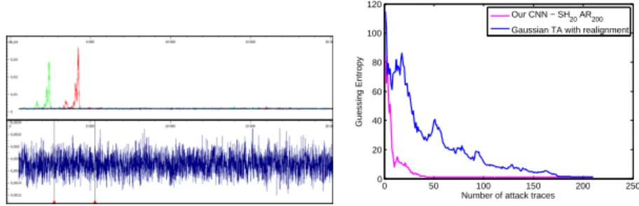
bytes leakages are completely misaligned. To illustrate the effect of this mis-alignment, the SNR characterizing the (aligned) first byte and the (misaligned) second byte are computed (according to the formula given in [4]) using a set of 150, 000 traces labelled by the value of the SubByte output (256 labels). These SNRs are depicted in the top part of Fig. 9. The SNR of the first byte (in green) detects a quite high leakage, while the SNR of the second byte (in blue) is nulli-fied. A zoom of the SNR of the second peak is proposed in the bottom-left part of Fig. 9. In order to confirm that the very low SNR corresponding to the second byte is only due to the desynchronization, the patterns of the traces correspond-ing to the second byte have been resynchronized uscorrespond-ing a peak-detection-based algorithm, quite similar to the one applied for the experiments of Sec. 5.1. Then the SNR has been computed onto these new aligned traces and has been plot in red in the top-left part of Fig. 9; this SNR is very similar to that of the first byte. This clearly shows that the leakage information is contained into the trace but is efficiently hidden by the jitter-based countermeasure.
We applied the CNN approach onto the rough set of traces (without any alignement). First, a 2, 500-long window of the trace has been selected to input CNN. The window, identified by the vertical cursors in the bottom part of Fig. 9, has been selected to ensure that the pattern corresponding to the leakage of the second byte is inside the selection. At this step, it is important to notice that such a selection is not at all as meticulous as the selection of PoIs required by a classical TA approach. The training phase has been performed using 98, 000 labelled traces; 1, 000 further traces have been used for the validation set. We performed the training phase over a desktop computer equipped with an Intel Xeon E5440 @2,83GHz processor, 24Gb of RAM and a GeForce GTS 450 GPU. Without data augmentation each epoch took about 200s.17The training stopped after 25 epochs. Considering that in this case we applied an early-stopping strat-egy that stopped training after 20 epochs without validation loss decrement, it means that the final trainable weights are obtained after 5 epochs (in about 15 minutes). The results that we obtained are summarized in Table 4. They prove not only that our CNN is robust to the misalignment caused by the jitter but also that the DA technique is effective in raising its efficiency. A comparison between the CNN performances and the best results we obtained over the same dataset applying the realignment-TA strategy in the right part of Fig. 9. Beyond the fact that the CNN approach slightly outperforms the realignment-TA one, and considering that both case-results shown here are surely non-optimal, what is remarkable is that the CNN approach is potentially suitable even in cases where realignment methods are impracticable or not satisfying. It is of partic-ular interest in cases where sensitive information does not lie in proximity of peaks or of easily detectable patterns, since many resynchronization techniques are based on pattern or peak detection. If the resynchronization fails, the TA approach falls out of service, while the CNN one remains a further weapon in the hands of an attacker.
17
raising to about 2, 000 seconds when SH20DA200 data augmentation is performed (data are augmented online during training)
0 50 100 150 200 250 0 20 40 60 80 100 120
Number of attack traces
Guessing Entropy
Our CNN − SH20 AR200
Gaussian TA with realignment
Fig. 9: Top Left: in green the SNR for the first byte; in blue the SNR for the second byte; in red the SNR for the second byte after a trace realignment. Bottom Left: a zoom of the blue SNR trace. Right: comparison between a Gaussian template attack with realignment, and our CNN strategy, over the modern smart card with jitter.
SH0AR0 SH10AR100 SH20AR200 a b 35.0% 1.1% 12.5% 1.5% 10.4% 2.2% c d 1.2% 137 1.3% 89 1.8% 54
Table 4: Results of our CNN over the modern smart card with jitter.
Conclusions
In this paper we have proposed an end-to-end profiling attack approach, based on the CNNs. We claimed that such a strategy would be robust to trace misalign-ment, and we successfully verified our claim by performing CNN-based attacks against different kinds of misaligned data. This property represents a great prac-tical advantage compared to the state-of-the-art profiling attacks, that require a meticulous trace realignment in order to be efficient. It represents also a solution to the problem of the selection of points of interest issue: CNNs efficiently man-age high-dimensional data, allowing the attacker to simply select large windows. In this sense, the experiments described in Sec. 5.2 are very representative: our CNN retrieves information from a large window of points instead of an almost null instantaneous SNR. To guarantee the robustness to trace misalignment, we used a quite complex architecture for our CNN, and we clearly identified the risk of overfitting phenomenon. To deal with this classical issue in machine learning, we proposed two Data Augmentation techniques adapted to misaligned side-channel traces. All the experimental results we obtained have proved that they provide a great benefit to the CNN strategy.
In machine learning domain, the Data Augmentation is often used to balance the class distribution of the training set, i.e. to make the training set contain the same number of data for each class. Used in this way it could provide further benefits to attacks that target unbalanced sensitive variables (e.g. the Hamming weight of a variable). The analysis of such benefits is left for future works, to-gether with the proposal of other deforming functions for the DA that could
simulate other random phenomena due to the acquisition noise and to other countermeasures. Another path for future works could consist in analysing the benefits CNNs might provide in presence of the masking countermeasure.
Acknowledgements
This work has been partially funded by the H2020-DS-LEIT-2016 project RE-ASSURE. The authors would like to thank Charles Guillemet for the fruitful discussions about this work.
References
1. Keras library. https://keras.io/.
2. Sonia Bela¨ıd, Jean-S´ebastien Coron, Pierre-Alain Fouque, Benoˆıt G´erard, Jean-Gabriel Kammerer, and Emmanuel Prouff. Improved side-channel analysis of finite-field multiplication. In Cryptographic Hardware and Embedded Systems - CHES 2015 - 17th International Workshop, Saint-Malo, France, September 13-16, 2015, Proceedings, pages 395–415, 2015.
3. Christopher M.. Bishop. Pattern recognition and machine learning. Springer, 2006. 4. Eleonora Cagli, C´ecile Dumas, and Emmanuel Prouff. Kernel discriminant analysis for information extraction in the presence of masking. In International Conference on Smart Card Research and Advanced Applications, pages 1–22. Springer, 2016. 5. Suresh Chari, JosyulaR. Rao, and Pankaj Rohatgi. Template attacks. In
Bur-ton S. Kaliski, Cetin K. Koc, and Christof Paar, editors, Cryptographic Hardware and Embedded Systems - CHES 2002, volume 2523 of Lecture Notes in Computer Science, pages 13–28. Springer Berlin Heidelberg, 2003.
6. Omar Choudary and Markus G Kuhn. Efficient template attacks. In Smart Card Research and Advanced Applications, pages 253–270. Springer, 2014.
7. Christophe Clavier, Jean-S´ebastien Coron, and Nora Dabbous. Differential power analysis in the presence of hardware countermeasures. In C¸ etin Kaya Ko¸c and Christof Paar, editors, Cryptographic Hardware and Embedded Systems - CHES 2000, Second International Workshop, Worcester, MA, USA, August 17-18, 2000, Proceedings, volume 1965 of Lecture Notes in Computer Science, pages 252–263. Springer, 2000.
8. Jean-S´ebastien Coron and Ilya Kizhvatov. An efficient method for random de-lay generation in embedded software. In Cryptographic Hardware and Embedded Systems-CHES 2009, pages 156–170. Springer, 2009.
9. Jean-S´ebastien Coron and Ilya Kizhvatov. Analysis and improvement of the ran-dom delay countermeasure of ches 2009. In International Workshop on Crypto-graphic Hardware and Embedded Systems, pages 95–109. Springer, 2010.
10. Thomas M Cover and Joy A Thomas. Elements of information theory. John Wiley & Sons, 2012.
11. Fran¸cois Durvaux, Mathieu Renauld, Fran¸cois-Xavier Standaert, Loic van Oldeneel tot Oldenzeel, and Nicolas Veyrat-Charvillon. Efficient removal of random delays from embedded software implementations using hidden markov models. In Inter-national Conference on Smart Card Research and Advanced Applications, pages 123–140. Springer, 2012.
12. R. A. Fisher. The use of multiple measurements in taxonomic problems. Annals of Eugenics, 7(7):179–188, 1936.
13. Ian Goodfellow, Yoshua Bengio, and Aaron Courville. Deep Learning. MIT Press, 2016. http://www.deeplearningbook.org.
14. A. Graves, A. Mohamed, and G. E. Hinton. Speech recognition with deep recurrent neural networks. In IEEE International Conference on Acoustics, Speech and Signal Processing, ICASSP 2013, Vancouver, BC, Canada, May 26-31, 2013, pages 6645– 6649, 2013.
15. Geoffrey E. Hinton, Nitish Srivastava, Alex Krizhevsky, Ilya Sutskever, and Ruslan Salakhutdinov. Improving neural networks by preventing co-adaptation of feature detectors. CoRR, abs/1207.0580, 2012.
16. Gabriel Hospodar, Benedikt Gierlichs, Elke De Mulder, Ingrid Verbauwhede, and Joos Vandewalle. Machine learning in side-channel analysis: a first study. Journal of Cryptographic Engineering, 1(4):293–302, 2011.
17. Sergey Ioffe and Christian Szegedy. Batch normalization: Accelerating deep net-work training by reducing internal covariate shift. CoRR, abs/1502.03167, 2015. 18. Alex Krizhevsky, Ilya Sutskever, and Geoffrey E Hinton. Imagenet classification
with deep convolutional neural networks. In F. Pereira, C. J. C. Burges, L. Bottou, and K. Q. Weinberger, editors, Advances in Neural Information Processing Systems 25, pages 1097–1105. Curran Associates, Inc., 2012.
19. Yann LeCun, Yoshua Bengio, et al. Convolutional networks for images, speech, and time series. The handbook of brain theory and neural networks, 3361(10):1995, 1995.
20. Henry W Lin and Max Tegmark. Why does deep and cheap learning work so well? arXiv preprint arXiv:1608.08225, 2016.
21. Houssem Maghrebi, Thibault Portigliatti, and Emmanuel Prouff. Breaking cryp-tographic implementations using deep learning techniques. In International Con-ference on Security, Privacy, and Applied Cryptography Engineering, pages 3–26. Springer, 2016.
22. Stefan Mangard. Hardware countermeasures against dpa–a statistical analysis of their effectiveness. In Topics in Cryptology–CT-RSA 2004, pages 222–235. Springer, 2004.
23. Zdenek Martinasek, Jan Hajny, and Lukas Malina. Optimization of power analysis using neural network. In International Conference on Smart Card Research and Advanced Applications, pages 94–107. Springer, 2013.
24. Zdenek Martinasek and Vaclav Zeman. Innovative method of the power analysis. Radioengineering, 22(2):586–594, 2013.
25. Sei Nagashima, Naofumi Homma, Yuichi Imai, Takafumi Aoki, and Akashi Satoh. Dpa using phase-based waveform matching against random-delay countermeasure. In Circuits and Systems, 2007. ISCAS 2007. IEEE International Symposium on, pages 1807–1810. IEEE, 2007.
26. Vinod Nair and Geoffrey E Hinton. Rectified linear units improve restricted boltz-mann machines. In Proceedings of the 27th international conference on machine learning (ICML-10), pages 807–814, 2010.
27. Lutz Prechelt. Early Stopping — But When?, pages 53–67. Springer Berlin Hei-delberg, Berlin, HeiHei-delberg, 2012.
28. Werner Schindler, Kerstin Lemke, and Christof Paar. A stochastic model for dif-ferential side channel cryptanalysis. In International Workshop on Cryptographic Hardware and Embedded Systems, pages 30–46. Springer, 2005.
29. F. Schroff, D. Kalenichenko, and J. Philbin. Facenet: A unified embedding for face recognition and clustering. In IEEE Conference on Computer Vision and Pattern Recognition, CVPR 2015, Boston, MA, USA, June 7-12, 2015, pages 815–823, 2015.
30. Patrice Y Simard, David Steinkraus, John C Platt, et al. Best practices for convo-lutional neural networks applied to visual document analysis. In ICDAR, volume 3, pages 958–962. Citeseer, 2003.
31. Michael Tunstall and Olivier Benoit. Efficient use of random delays in embedded software. In IFIP International Workshop on Information Security Theory and Practices, pages 27–38. Springer, 2007.
32. Jasper GJ van Woudenberg, Marc F Witteman, and Bram Bakker. Improving differential power analysis by elastic alignment. In Cryptographers Track at the RSA conference, pages 104–119. Springer, 2011.
33. Nicolas Veyrat-Charvillon, Marcel Medwed, St´ephanie Kerckhof, and Fran¸ cois-Xavier Standaert. Shuffling against side-channel attacks: A comprehensive study with cautionary note. In International Conference on the Theory and Application of Cryptology and Information Security, pages 740–757. Springer, 2012.
34. Sebastien C Wong, Adam Gatt, Victor Stamatescu, and Mark D McDonnell. Un-derstanding data augmentation for classification: when to warp? In Digital Image Computing: Techniques and Applications (DICTA), 2016 International Conference on, pages 1–6. IEEE, 2016.
35. Shuguo Yang, Yongbin Zhou, Jiye Liu, and Danyang Chen. Back propagation neu-ral network based leakage characterization for practical security analysis of cryp-tographic implementations. In International Conference on Information Security and Cryptology, pages 169–185. Springer, 2011.
A
Historical Overview of Neural Networks
The main blocks of NN models exist since the early 1980’s but, for a long time, other methods (e.g. Support Vector Machines with kernels) have been preferred since they lead to unique solutions. The situation has recently changed with the increasing of both the size of the training database (e.g. available in the clouds) and the computing performances (e.g. deployment of very fast GPUs for parallel computing), and also thanks to technical improvements (e.g. the introduction of the dropout regularization technique [15] and the introduction of the REctified Linear Unit activation function [26]). They have brought out the NNs, putting them forward in the 21st century. They, for instance, play a central role in face recognition [29], image classification [18] or speech recognition [14]. In the field of images, the CNNs [19] stand out for their performances. Basically, a CNN differs from the most ordinary NN, the so-called Multi-Layer Perceptron (MLP), from the fact that CNNs share parameters across space: instead of assigning to each part of the image some parameters to be optimised, the CNNs exploit smalls vectors of weights as convolutional filters, applying the same weights over the whole image. The constraint given by the sharing parameters leads the network to learn shift-invariant features: for image recognition it makes perfect sense, since shifting the image pixels does not make the subject change (e.g. a shifted image of a car keeps being an image of a car). The excellent performances of
CNNs in image recognition [18] demonstrate that such an architecture also man-ages others image invariant-deformations, e.g. the scaling, the rotation, etc.
B
Discussion about Software Countermeasures
The goal of the experiences performed in in Sec. 4 was to verify the shift-invariance property claimed by the CNN architecture. We achieved this objective by considering the case of a simple countermeasure, the uniform RDI, which con-sists in injecting shifts in side-channel traces. We remark that this kind of coun-termeasure is nowadays considered defeated, e.g. thanks to resynchronization by cross-correlation [25]. The complexity of the state-of-the-art resynchroniza-tion techniques strongly depends on the variability of the shift. When the latter variability is low, i.e. when attacks are judge to be applicable, multiple random delays are recommended. It has even been proposed to adapt the probabilis-tic distributions of the random delays to achieve good compromises between the countermeasure efficiency and the chip performance overhead [8, 9]. Attacks have already been shown even against this multiple RDI kind of countermeasures, e.g. [11]. The latter attack exploits some Gaussian templates to classify the leakage of each instruction; the classification scores are used to feed a Hidden Markov Model (HMM) that describes the complete chip execution, and the Viterbi algo-rithm is applied to find the most probable sequence of states for the HMM and to remove the random delays. We remark that this HMM-based attack exploits Gaussian templates to feed the HMM model, and the accuracy of such templates is affected by other misalignment reasons, e.g. clock jitter. We believe that our CNN approach proposal for operation classification, is a valuable alternative to the Gaussian template one, and might even provide benefits to the HMM per-formances, by e.g. improving the robustness of the attack in presence of both RDI and jitter-based countermeasures. This robustness w.r.t. of misalignment caused by the clock jitter is analysed in Sec. 5.