Design of an electrohydraulic servovalve.

FEB 3 1965

DESIGN OF AN ELECTROHYDRAULIC SERVOVALVE

By

Robert Harley Maskrey

S.B., Massachusetts Institute of Technology (1963)

SUBMITTED IN PARTIAL FULFILMENT OF THE REQUIREMENTS FOR THE DEGREE OF

MASTER OF SCIENCE at the

MASSACHUSETTS INSTITUTE OF TECHNOLOGY

Signature Certified by Accepted December, 1964

Signature redacted

Department of Mechanical Engineering, Decemb r, 1964

Signature redacted

I

Thesis Supervisor

Signature redacted

by . . . . . ....

Chairman, Departmental Committee on Graduate Students

Robert H. Maskrey

Submitted to the Department of Mechanical Engineering December 1964, in partial fulfillment of the requirements for the degree of Master of Science.

ABSTRACT

A design for the first stage of an electrohydraulic servovalve

is presented. The proposal consists of a voice-coil type electro-mechanical actuator, a sliding plate valve, and a pure fluid jet amplifier, The design problems of a no-hysterisis actuator were considered, and an acceptable device was constructed. The

important parameters involved in designing a pressure controlled pure fluid amplifier operating on hydraulic oil were investigated analytically and experimentally. A satisfactory model was built on

the basis of the findings. The two elements were connected with a sliding plate valve and a graphical method was employed to predict the output. The static behavior of the system agreed well with predicted resulted, but the dynamic response was considerably poorer than that of the actuator alone.

Thesis Supervisor: Herbert H. Richardson

Title: Associate Professor of Mechanical Engineering

-i-ACKNOWLEDGMENT

I would like to express my sincere appreciation to my advisor, Professor H. H. Richardson, for his invaluable guidance in this undertaking, and the preparation of this thesis.

In addition thanks is also offered to the other members of the Engineering Projects Laboratory for their constructive

criticism and helpful suggestions, and to my wife, Sandy, for typing both-the rough and final draffs of the thesis.

This thesis was supported in part by the United States Air Force under contract 33(657)-7535 and sponsored by the Division of Sponsored Research of Massachusetts Institute of Technology.

1-2 Block Diagram of Proposed First Stage 7

2-1 Cylindrical Magnetic Field 14

2-2 Magnetic Circuit 14

2-3 Equivalent Electiic Circuit ₁₅

2-4 Magnet Dimensions 15

2-5 Magnetization Curve for S.A. E. 10-10 Cold-Rolled 17

Mild Steel

2-6 Air Gap Permeances 19

2-7 Forces on Moving Coil 19

2-8 Voice Coil Actuator - Test Configuration 26

2-9 Test Apparatus Schematic 27

2-10 Magnet Saturation Curve 29

2-11 Frequency Response 30

2-12 Frequency Response 31

2-13 Frequency Response 32

2-14 Frequency Response 33

2-15 Effect of M, k, B, and I On "Break Point" 35

2-16 Voice Coil Frequency Response 37

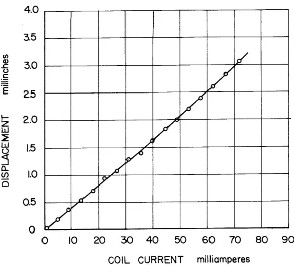
2-17 Coil and Valve Plate Frequency Response 38

3-1 Fluid Jet Amplifier Terminology 43

3-2 Turbulent Jet Velocity Profile 46

3-3 Two-Dimensional Laminar Jet Velocity Profile 49

3-4 Control Flow Components 51

3-5 Typical Input Source Characteristics 51

3-6 Fluid Jet Amplifier - Test Model 55

3-7 Apparatus 55

3-8 Control Flow as a Function of Ps and Lateral Setback 58

3-9 Effect of Higher Mean Flow 59

3-10 Right Hand Control Port Demand Curve 61

3-11 Control Volume for Jet Deflection

63

3-12 Amplifier Nozzle Discharge Coefficient as a Function 66

of Supply Pressure and Aspect Ratio

3-13 Deflected Jet Impinging on Receiver 68

3-14 Predicted Output Pressure Drop vs. Jet Deflection 71

and Receiver Width

3-15 No-Load Flow at One Receiver vs. Jet Deflection 73

and Receiver Width

3-16 Single Receiver Flow and Output Pressure as a Function 74 of Jet Deflection and Receiver Width

3-17 Influence of Receiver Spacing for TI Z 0.1 76 3-18 Pressure Recovery as a Function of Supply Pressure 79 3-19 Pressure Recovery as a Function of Aspect Ratio 80

3-20 Recovered Pressure as a Function of 82

3-21 Pressure Recovery as a Function of Receiver Shape 84

3-22 Models for Venting Study 85

3-23 Load Pressure vs. Control Pressure Difference for 85

Vented Models

3-24 Fluid Jet Amplifier Prototype 89

3-25 Control Port Demand Curve 91

3-26 Receiver and Load Pressures as a Function of Control 92 Pressure

4-1 Sliding Plate Valve 95

4-2 Valve Plate Opening 97

4-5 Loci of Possible Operating Points 103

4-6 Actual Operating Points 103

4-7 Predicted Control Pressure as a Function of Valve 104

Displacement for Ps = 300 psi , Pc= 100 psi, Xm = . 005 in

4-8 Predicted Load Pressure as a Function of Valve 105 Displacement for Ps= 300 psi, Pc = 10 psi,

Xmz .005 in

4-9 Static Test Apparatus 106

4-10 Receiver and Load Pressures as a Function of Valve 107

Displacement and Control Pressure

4-11 Four-Way Valve Characteristics for Fluid Amplifier 109 and Plate Valve, PC= 15 psi

4-12 Four-Way Valve Characteristics for Fluid Amplifier 110

and Plate Valve , PC' 10 psi

4-13 Exploded View of First Stage Package 113

4-14 Photo of Complete First Stage Package 114

4-15 Ram Type Load 115

4-16 Frequency Response of Valve 116

B-1 Torque Motor Amplifier 127

B-2 Audio Amplifier 127

B-3 Complementary - Symmetry Amplifier 129

B-4 Amplifier Frequency Response 131

B-5 Amplifier Input Output Characteristics 132

B-6 Transistor Amplifier and Power Supply 133

B-7 Amplifier with Feedback 129

B-8 Circuit Diagram 135

NOMENCLATURE

A

Art

magnetic field strength

b

nominal coil diameter diameter of magnet pole

D. C. magnet current

L current into coil

mechanical spring rate coil length

length of current carrying wire downstream receiver distance number of turns

air gap permeance control supply pressure load pressure

PS jet supply pressure receiver pressure

2. pressure in control port

Q

~

Q M load flow

Qr.e

-W

X

Ye

YQ

0(o

A.-,04)

/0

/0

Subscript o refers to initial condition or static respones Subscript 1 and 2 refers to right and left sides of amplifier

-vii-receiver separation

coil and valve displacement axial setback

length of flow establishment region (Albertson) lateral setback

wave number = Yp7 (Pai) jet deflection

Gaussian integral flux density

permeability of air 3. 2 maxwells / ampturn in.

hydraulic oil viscosity

wire density - mass / unit length material density

hydraulic oil density

TABLE OF CONTENTS

Abstract

Acknowledgments ii

List of Illustrations iii

Nomenclature vi

I. INTRODUCTION AND PROPOSAL I

1.1 Introduction 2

1. 2 Proposed Design 5

II. ELECTROMECHANICAL TRAN3DUCER 9

2.1 Specifications 12

2. 2 D. C. Magnet 12

2. 3 Moving Coil 22

2. 4 Prototype Model and Testing 24

III. FLUID JET AMPLIFIER 39

3.1 Amplifier Description 41 3. 2 Power Jet 45 3. 3 Control Region ₄₈ 3. 3.1 Characteristics 50 3. 3. 2 Stability 50 3. 3. 3 Geometry ₅₃ 3. 3. 4 Experimental Equipment 54 3. 4 Jet Deflection ₆₂ 3. 5 Receiver Ports ₆₅

3. 6 Extraneous Effects 86 3. 7 Fluid Jet Amplifier Model 88

IV. SYSTEM 93

4.1 Plate Valve 94

4. 2 Valve Plate-Moving Coil Combination 96

4. 3 Load Matching 98

4. 4 Static Valve Test 101

4. 5 Complete First Stage 112

V. SUMMARY AND CONCLUSIONS 118

5. 1 Summary 119

5. 2 Conclusions 122

Appendix A - Coil Wire 123

Appendix B - Amplifier and Power Supply 125

I INTRODUCTION AND PROPOSAL

1. 1 Introduction

The recent major advances in space technology and industrial controls have brought about new requirements in mechanical hardware. Because of high force, high power, low weight and volume and high reliability requirements of particular control systems, especially in space flight, fluid power control is often chosen to provide necessary mechanical actuation. The requirements of a typical actuating system would be for a high stiffness, high frequency, high force device that could accurately be controlled from low power electrical signals

emanating from various transducers and computer operated controllers. The former requirements would call for a hydraulic type of actuator, cylinder-ram combination, while the latter specifies an electrical

device. _{Hence, some form of electrohydraulic actuator is called for} that would enable the coupling of these two systems. The resulting device is usually a 4 way hydraulic valve operated with an electrical signal and having an output valve pressure (or flow) proportional to the strength of the input signal.

Various such devices have been designed and produced for specific applications by several companies. The typical configuration of this type controller consists of a moving iron electro magnetic torque motor that translates the electrical input signal into a push-pull output displacement, a pair of flapper nozzle valves that serve to

convert the displacement into a sufficient pressure drop to energize a second stage of amplification. The second stage is a spool type

-3-four-way valve acting as the output stage and meeting the hydraulic control requirements.

The above type device combines the advantages of the electromechanical actuator and the hydraulic valve. The electro-mechanical actuator alone could not provide the required force, nor could it offer adequate stiffness and yet maintain a small size. At the same time the spool valve requires a relativly high force to

operate and needs a fairly stiff driving mechanism to counteract the transient and steady state valve forces. So, the combination of these two items requires an interim stage of amplification that is provided by the flapper nozzle valves. This type of actuator is

a two-stage electrohydraulic servovalve. A typical configuration

is given in figure 1.-1.

The advantages of this type actuation as indicated above are: 1) high stiffness - large resistance to force feedback from load.

2) high forces- limited only by the hydraulic source and pressure limitations of the hardware. 3) high response speeds - relatively high frequency possible for a mechanical device. 4) high power gain

-large hydraulic power changes possible for small input electrical signals. 5) compatibility - most signal sources are of electrical nature since current or voltage is easier to handle, thus the device is readily adapted to many uses.

There are disadvantages, too, to this type of device.

1) High manufacturing tolerances, hence high cost of finished product.

This is the principal limitation to wider industrial acceptance. 2) Steady state leakage. Two stage valves as described generally

First Stage

Input

I

Torque

i

Motor

---

-Flapper

Nozzle

Valves

Ps

2

__-__

Ps

₂

Vave.Pk

Pos it io n

Valve

P

e

Spring

Ps

AID_

Second Stage

To Load

I

-5-have some quiescent flow through the first stage amplifier even when the spool is in its neutral position. Additionaly, in the torque motor, there is also a quiescent current present when at rest. 3) Hysteresis

-the primary cause of hysteresis in -the electrohydraulic servovalve is the use of moving iron type transducers.

The purpose of this investigation is to propose and examine a device that will eliminate the hysteresis problem, reduce the manu-facturing costs and yet maintain the same advantages presently enjoyed

by existing electrohydraulic valves.

Much of the above emphasis is on the electromechanical transducer and the first amplifier, or the first stage of the valve, so the primary concern will be to revise this part of the total valve ignoring the second stage or spool.

The necessity of reducing manufacturing total cost needs

not be explained. It would greatly expand the possible uses for hydraulic actuation. Hysteresis is perhaps not so obvious an ill. In any control

system with a closed loop where hysteresis is present, there exists the possibility for limit cycle oscillation. Since there can be output with no input, hysteresis leads to error even in open loop. In addition, the phase shift produced by hysteresis may be undesireable.

1. 2 Proposed Design

The device proposed to act as a first stage of a two stage servovalve uses a voice-coil type electromechanical actuator and a fluid-jet amplifier. The actuator provides a translation from the current input to a mechanical motion. This motion in turn controls

the opening of a pair of variable orifices. The orifices regulate the control pressures and flows supplied to the control ports of a pressure

controlled proprotional pure fluid amplifier. The output of the amplifier is a pressure that serves to operate a conventional spool valve. In essence this first stage is now a two stage device by itself. Figure 1-2 gives a schematic of the operation.

The optimal design of an electromechanical actuator is considered, within the limits of geometry, input current, output dis-placement, and natural frequency. For a given magnet material and mass load, the design is over specified, so the problem was consider-ed to maximize the natural frequency, retaining the other requirements.

The problems of operating a fluid jet amplifier at low

-Reynolds number conditions are considered. The effects of control port geometry and _{supply pressure on the input characteristics are} investigated. _{A study of receiver port location and geometry was} carried out in order to maximize the pressure gain of the device

without sacrificing flow gain. A comparison of viscous-incompressible fluid jet amplifiers with preumatic high-Reynolds number amplifiers is given and some limitations of the device are spelled out.

A sliding plate valve is designed to adequately couple the

actuator and the amplifier. A method for prescribing input devices to the amplifier is demonstrated. _{Impedance requirements and}

stability problems that determine the operating characteristics of the valve are considered.

A transistor amplifier for operating the valve was designed

VOLTAGE

SIGNAL

PC

Electronic

_{Voice Coil}

_Variable

Amplifier

Actuator

x

Or ices

CURRENT DISPLACEMENT

AP

AQ

p

Fluid Jet

SAmplif ier

Spool

Valve

BLOCK DIAGRAM

OF PROPOSED

FIRST STAGE

actuator.

Static and dynamic characteristics of the complete first stage package are presented, and its operation in a closed loop system is evaluated.

-9-II ELECTROMECHANICAL TRANSDUCER

-II ELECTROMECHANICAL TRANSDUCER

The most useful electromechanical device for this applicat-ion is a transducer that translates a current input into a positapplicat-ion output. Since a linear spring can be used for reducing a force output to a displacement, the problem then becomes one of causing a

bidirectional current to produce a bidirectional proportional force. The three most common ways of meeting this end are through variable reluctance magnetic means, electrostatic means and through the force exerted on a conductor by a magnetic field.

The selection of the proper device depends on the use or type of performance it will be required to attain. The following factors should be considered and their relative importance evaluated to aid in the selection of a device; maximum force, maximum stroke, maximum current, weight of device, natural frequency or speed of response, maximum temperature rise allowable, type of motion desired (ie: torque or force), geometrical limitations, plus other inherent limitations peculiar to specific devices such as inductance or capacitance effects, hysteresis and quiescent currents.

The particular requirements in this case are for a no-hysteresis, high frequency actuator to meet specific stroke

require-ments. The first condition would automatically eliminate the moving iron device because of the hysteresis present in a fluctuating magnetic field. The last two conditions would call for a high force to obtain a high frequency (stiff spring) and yet keep an adequate stroke. The

-11-two conductors carrying a current is given by:

S

2iid

(2.1)

where is the length of each wire of distance apart d, and is the permeability of air. The force on a moving coil device is:

F1--=

R

where is again the length of wire carrying a current i and B is the magnetic flux density. The ratio of these two forces for the same current and wire length is:

(2. 3)

By limiting i to 100 ma. and specifying d to be one half the maximum

stroke or . 005 inches, letting Yo= 3. 2 maxwells/ampturn - in. and taking B to be one-quarter the maximum flux in a magnet or about

30 kilomaxwells/in 2 , the force ratio becomes

S10

This clearly limits the choice to the moving coil device, where if the limitations were size and not current, the electrostatic device would be comparable since it requires no constant magnetic field.

There are two popular configurations of the moving coil device. The first is the translating coil as in a loud speaker voice coil and the second is the rotating coil as in a d'Arsonval meter movement. Of these two, the voice coil seems the most efficient

since the rotating device requires a larger diameter to produce the same force, and only a portion of the coil is in the magnetic field at any time.

2. 1 Specifications

There must be some specific requirements for a typical actuator so the design parameters for the coil can be selected and

so the feasability of the particular design can be adjudged. The important specifications are size, natural frequency, displacement, and input signal requirements since these determine the properties of input and output appliances and applications. On the basis of existing torque motors, the following specifications were selected.

Maximum displacement * . 005 in Maximum current input * 100 ma Natural frequency 500 cps

Size .750 x .750 x .750 in

These requirements when coupled with other practical stipulations as temperature rise, available wires sizes, materials,

and power limitations define the actuator.

The voice coil actuator can be divided into two parts, the moving coil, its connections and spring, and the permanent magnet. The problem of optimally designing the permanent magnet will first be considered.

2. 2 D. C. Magnet

The function of the magnet is simply to provide a constant magnetic field in a gap of sufficient width and length to permit

operat-ion of the coil. For convenience a D. C. electromagnet was sub-stituded for the permanent magnet as the effect would be the same.

-13-as far as compactness and accessability is a cylindrical magnetic field as in figure 2-1. The geometry and properties of this design must be selected to maximize the flux density in the gap. For com-patibility with a suitable coil, the gap dimension of . 080 inches width

and . 250 inches length were chosen, with diameter to be a variable.

The magnetic circuit shown in figure 2-2 can be thought of as analogous to the electrical circuit of figure 2-3. The problem is one of minimizing the leakage permeance or maximizing the permeance of the air gap, similar to minimizing the load resistance and maximiz-ing the parallel resistance in the electrical circuit. At the same time, the permeance of the magnet itself must be a maximum while provid-ing the largest room possible for the D. C. coil. These conditions therefore specify the magnet geometry. To minimize the magnetic "resistance" of the magnet, the flux paths must be as short as possible and the cross sectional area as large as possible. At the

same time the area must be small to allow sufficient coil room. The path length is virtually fixed, so the cross sectional areas must be

equal and kept a minimum.

The equal area condition allows the following relations in dimensions from figure 2-4.

3 _(2.4)

4

4

d

_-

D.C. Coil

Space

Gap

Length

CYLINDRICAL MAGNETIC FIELD

5 2! 4 2'

MAGNETIC

Figure

Leakc

Mean Flux

Path

Useful

Flux

ge Flux

CIRCUIT

2-2

Gap

Width

Figure 2-1

F

A

I..

a4-g

i

b

h=.250"

MAGNET DIMENSIONS

Figure 2-4

EQUIVALENT ELECTRIC

CIRCUIT

Figure 2-3

c>

/7

And geometric compatibility allows these relations:

2A

d

2a

.750

+ C

-TE;D(2.7)

.2s;

The coil space is a cylinder with crossectional area a x c. For any given wire material the number of turns in this space varies inversely with the (diameter)2 and the current carrying capacity varies directly with (diameter)2. So, the product should be about constant independent of wire size. For a typical wire size there are 320 turns / in2 at 1 amp maximum current, so the magneto motive force is

N

=

=

20

- a-c.

amp-

4

rris

The material selected for the magnet is SAE 1010 mild cold-rolled steel and the magnetization curve is given in fugure 2-5. From this a typical maximum flux density in the steel is picked at 120 kmax/in2 . So the maximum flux at any place in the magnet is

>120

Wmax

1-0

-

4

because of the equal areas.

If Q is the total leakage and air gap permeance,then for the complete circuit, assuming that the permeance of steel is infinity,

N=

PT

p..

140

120

100

80

60

40

20

0

0.1

.2

.5

1.0

2.0

5.0

10

20

50

100 200 500

10

MAGNETIC

INTENSITY

MAGNETIZATION

Amp- turns

/

inch

CURVE

for

S.A.E. 10-10 COLD-ROLLED

MILD STEEL

FROM ROTERS Ref.(I)

co 0

E

_n

C/)

z

w

x

-It remains only to solve this equation for the proper geometry. From Roters(l) the permeance of the air gaps as indicated in figure 2-6 are given as such:

d( +q ) _{(2. 12a)}

R 63

-S L.A

+

j

i

.

(c)

R

~(d)

Adding parallel permeances,

r =P + RP * P4 k+ Ps- (2.13)

This cannot be easily solved, but by using the following series approximations:

+E) =+(2. 14a)

+2(

+i)

YLi= E\)- (E\+ ( \ (d)

where E is a small number, and applying to equations 2. 12a through

2. 12e the total permeance can be determined in terms of d, a, h, g,

and assorted constants, h and g are known and a is related to d from (2. 6), so equation (2.13) can be solved for d. Only terms of third order were kept in each unknown, so the final equation was seventh

-19-AIR GAP PERMEANCES

Fig. 2-6

L

olo

B

M

x

k

FORCES ON MOVING COIL

Figure 2-7

p,

order in d. The real practical root satisfying the equation is

Equation 2. 4 to 2. 7 can be solved for the entire geometry.

Using this geometry and an estimated mean flux path as shown in figure 2-2 combined with the figure 2-5, the total magneto-motive force can be calculated. Airgap and leakage permeances are as given in equations (2. 12a) to (2.12e) with the additional leakage permeance

FL d+2c (2.15)

d

This occurs through the coil windings and is used to calculate the flux through parts 4, 5, and 6. A brief table of the calculations is

given in table 1. The starting point for this estimation was that one part of the magnet had gone into saturation, saturation being approx-imately 120 kmax/in2 . These results indicate that the required force is 311 ampturns to produce a flux of 4. 0 kmax in the gap. But of this flux only the fraction proportional to P is actually useful

PT

.0-L =-2,32

Or, this is a flux density of: 13. 4 kmax/in2 in the air gap.

This not necessarily the ideal design of the D. C. magnet, since the best design would make the length of the gap as long as

PI

physically possible, to make - large, but for the imposed

limita-tions of . 250 inches gap length, this the maximum magnetic field.

The wire used for the coil winding is immaterial in theory (see appendix A) but is limited for practical reasons. Power supplies

TABLE I B kmpx/in2 H ampturns -in F ampturns 3. 92 x 10-1 1. 43 x 10-1 3. 8 x 10-2 6. 94 x 10-2 1. 25 x 10-1

4.

0 (

4. 426 q

116.0

67.

9.

68. 6

1)

Max

4

4=

is smallest area available, so

2)

0 6

&

4

4

3)

P5

₌

₆

4L

1

typically supply current in the 1 amp range so sufficiently small wire should be chosen to keep the current in this range.

2. 3 Moving Coil

Next to be considered is the moving coil, subject to the same geometry limitations as the magnet air gap. The function of the coil is to provide a large force or displacement at a high frequency for a fixed current input in a fixed magnetic field. With a configura-tion as shown in figure 2-7, balancing the forces on the bobbin gives:

NTT

D L

where D is a mean coil diameter, and k is the elastic constant of the spring. The static current to position transfer function is then:

X

(2. 17)

while the natural frequency for this second order system is given by

WK = _{(2. 18)}

The mass is in three parts, the load which remains constant, the bobbin which depends on geometry and the coil itself which depends on geometry and wire properties. The spring mass can be lumped in with the load mass

Vnt

given by

06 IT (L * s(2.20)

where /0 is the density of the bobbin material. The second term comes from the end caps. The wire mass is

we is th wi m asD (2.21)

-23-Natural frequency is then

LU k ol(2.22)

nAt /061 (L+) - +Ow

This does not have a practical maximum, but as N gets very large it is inversely proportional to the wire density. A large number of

turns of low density wire will maximize the speed of response.

A second problem of consideration is heating in the coil,

or required power. For a given current, power depends on the total resistance of the coil. This resistance, for a wire of diameter d and resistivity /0 is

(2. 23)

Similarly the wire density per unit length fu is given by

OCA

4

/0-JT(2.24)

if ) is the actual wire density. Combining the two:

R

-M-mpo,

Since it is desireable from above to minimize both R and /O , a figure of merit for the coil wire would then be a low

,p.

all commercially available wire materials Aluminum posesses this minimum, with Copper second.

The maximum expected speed of response, or natural frequency, would then occur for an aluminum wire coil. If N is

assumed very large, an asymptotic natural frequency can be calculat-ed. For N large:

calculated in table 2. In addition the expected natural frequency from equation 2. 22 is shown and the coil resistance. From this table, the aluminum coil material would be superior. Unfortunately for the present case, both of these considerations, bobbin and load, are important. Several wire materials had to be tested to determine

an adequate coil.

2. 4 Prototype Model and Testing

For the prototype model a three leaved brass spring provided both the required translational spring stiffness as well as a rigid radial support for the coil. Figure 2-8 shows the complete magnet and moving coil assembly. The fiber spacers are for testing purposes only and do not appear on the final model.

For the test series on the actuator, a linear variable differential transformer was connected to the moving coil. When the output signal was demodulated, this provided a position pickoff for the coil and the L. V. D. T. provided a mass load to the coil. Power was supplied to the D. C. magnet from a variable current source, as described in Appendix B. The signal to drive the coil was provided by a low frequency oscillator and amplified by a transistorized D. C. amplifier, also described in the Appendix. A diagram of the apparatus as used to obtain frequency response

TABLE II

Coil Wire # Turns Resistance

Asymptotic a. cps Expected Wv cps Measured WJb cps #38 Al 437 41 X 440 240 110 #41 Cu 427 43 C 345 220 128 #37 Cu 302 13. 5.a 216 175 85 (Ji

4 TIMES ACTUAL SIZE

D.C. Magnet

~'

Windings

Moving Coil

and

Windings

Spring

VOICE COIL ACTUATOR

-

TEST

CONFIGURATION

Figure 2-8

Brass

Spacer

Phenol ic

Spring

Supports

-27-Low Fre q.

Oscillator

v

Os cillator

Amplif W?

Power

I

Magnet &

x

supply

Coi

L..DT

D emodulator

T o

---'

Scope

TEST APPARATUS

SCHEMATIC

Figure 2-9

After a period of testing to eliminate the major apparatus flaws, the first major test to be conducted was that to determine magnet saturation. To operate the magnet most effeciently it should be in saturation, thus the magnetic field in the gap is a maximum, but if is is too far in saturation most of the input energy is going into heat and not into gap energy. Further, if the magnet is saturated,

any hysteresis loop due to the small demagnetizing field produced by the moving coil will have negligible effect.

To determine this curve experimentally, a sinusoidal signal with a frequency of 10 cycles per second, far below the coil natural frequency, was fed to the voice coil. The resulting amplitude of oscillation was then measured at various levels of current in the

D. C. magnet. Figure 2-10 gives these results plotted against both current and ampturns. From this test the indication is that a good operating point would be just above one amp, and the remaining tests were carried out at this level.

The next series of tests were frequency response tests performed under approximately similar input currents. Sinusoidal input current was varied from about 2 cps. up to the level that motion was no longer resolvable. Several values of spring rate were used and the magnet coil wire, both material and number of turns was

varied. The output displacement was plotted versus input current on an oscilloscope, and the resulting lissajous figure gave the amplitude and phase of the output. Most of the results from these tests are given in figures 2-11 through 2-14. The two important pieces of information from these response curves are the "gain",

-29-0 B 0 0 0 0 0 0 0 0 0 0 0 0 0, 0 0 00 0 00 0 0 0 0 0 0 0 0 0 0 0

a

3cifldAJV

MAGNET

F

SATURATION

igure

2-10

CURVE

Q

E

0j

z

E

Q

-

20

5

10

20

FREQUENCY

50

100

cps

RESPONSE

Figure 2-11

o

10

E

>2

MQ2

0.1

*' 37 Copper Wire

302 turns

.002 in Spring

1

2

5

10

20

50

100

500

FREQUENCY

cps

a_

180

I

2

500

-31-2

5

10

20

FREQUENCY

50

100

cps

RESPONSE

Figure 2-12

a

E

.5

I

-0.2

w

-. 05

0.02

0.01

0

90

w

180

I

2

500

"37

Copper Wire

302 turns

.003 in Spring

1

2

5

10

20

50

100

500

FREQUENCY

cps

10

5

10

20

50

100

200

500

cps

VOICE COIL FREQUENCY

RESPONSE

Figure

201

D

E

5

2

41 Copper Wire

427 turns

.002 in Spring

2

5

10

20

50

100

200

500

FREQUENCY

cps

.5

.2

.1

0

90

180

I

2

2-13

-33-5

IC

20

FREQUENCY

5

10

20

FREQUENCY

Figure

50

100

cps

50

100

cps

RESPONSE

2-14

20

10

2

E

III

AT

37Copper Wire

344 turns

.002 in Spring

<0.2

a[

1

2

w

9d

500

500

18Cf

1

2

or input/output ratio, and the natural frequency of oscillation. Ideally, the input/output ratio could be adjusted to the desired level

of 5 mill/100 ma by simply varying the spring rate, with a subsequent change in natural frequency. For a given coil these two quantities

should depend only on the value of the spring constant, according to the relations in equations 2. 17 and 2. 18. Combining these two gives:

2W Nz

So, a plot of input/output versus natural frequency for several values of spring rate should lie along the line

r 1/0

-2

Yv

wA

coiis-.

where the constant varies only for coil properties. Good correlation is found when these plots are made with springs . 002 inches and . 003

inches thick. Unfortunately only two points for a given coil could be determined since the stiffer springs had such a small displacement that it could not be recorded accurately, and the softer springs produced limiting of the coil motion, plus a marked friction effect due to inadequate radial stiffness. Figure 2-15 gives these plots for several coils with an indication of what effects changing the various

coil parameters would have.

From this information, the natural frequency for the coil operating at the desired displacement can be ascertained. A

com-parison of this result with the previously predicted results is given in table 2.

-35-10

20

50

100

200

FREQUENCY

cps

EFFECT OF

M, k,

B,

and

.

ON

"BREAK POINT"

Figure 2-15

10

5

2

E

-c

w

inc.k

"

Al

increasing

M

"41Cu

437

Cu

dec.

"41 Cu

orB

37Copper

.2

.1

500

could be constructed and still retain the desired strength. These were made and were tested, not with brass springs as previously, but with a model of the final plate valve in place. These response curves are in figures 2-16, 2-17. While the performance of these coils was better, it is not reflected in the response curve as the dynamic loading was greater, due to the higher mass of the plate

valve.

Although the Aluminum coil did show better response gain characteristics than the #37 Copper and #44 Copper coils, many

dificulties occured that would not recommend its final usage. First, the wire appeared much more brittle than the relatively ductile copper, probably because of the manufacturing method. Mechanical failure due to flexing in the higher frequency tests was common. A second manufacturing headache occurs with the joining of the aluminum wires. While copper can easily be soldered,

-luminum cannot, and the high temperature soldering methods

us-ually applied to the aluminum would melt the wire.

The coil chosen for the final model was the #42 Copper,

Teflon coated 689 turns, and weighing unloaded approximately 2 grams. It has a resistance of 82 ohms and an inductance of 2 millihenries.

-37-20

10

5

10

20

VOICE COIL

50

100

200

cps

FREQUENCY RESPONSE

Figure 2-16

0

E

05

E

.5

S2

0

90

uj

180

1

2

500

38 Aluminum Wire

437 turns

Plate Valve Spring

1

2

5

10

20

50

100

200

500

2C

IC

5

2

1

2

COIL AND

5

10

20

VALVE PLATE

50

100

cps

FREQUENCY RESPONSE

Figure

E

-c

42 Copper Wire

689 turns

Plate Valve Spring

1

2

5

10

20

50

100

200

500

FREQUENCY

cps

a-.5

2

0

'90

w

500

I

2-17

III FLUID JET AMPLIFIER

Pure fluid jet devices have been the subject of much investigation in recent years, as a logic and control element. The first reference to their use was by Coanda(2 _{) in 1933, and very little}

came of his ideas until 1960 when both Diamond Ordnance Fuze Laboratories and Massachusetts Institute of Technology initiated woek on pure fluid logic. Work is presently being done by a large number of private concerns and institutions related to applications.

The no moving parts advantage offered by pure fluid amplification promises a longer life, higher reliability, easier operation under adverse conditions, and faster speed of response than present mechanical control elements. Unfortunately the apparent

simplicity of these devices does not pertain to a mathematical re-presentation. _{It is virtually impossible to adequately predict the} operation or even a simple transfer functions for a full range of operating conditions. While this is detrimental, it by no means

eliminates their use as a control element, since they can be classified according to various geometry and fluid properties. The characteristics can then be empirically determined for each classification, much like transistors, their electronic equivalent.

Fluid amplifiers fall into several basic classifications, according to the type of control and method of operation. Analog and digital are the two methods of amplification, and they can be either pressure or momentum controlled. Digital devices are

-41-used for logic circuits. Generally they operate on the Coanda principle of a jet attaching to a downstream paralled wall. Pro-portional amplifiers, used as control elements, depend on a jet being deflected toward or away from one of a pair of receivers, without attachment. Momentum control uses one or two control jets to deflect a third power jet by impinging perpendicular to it. Pressure control depends on a pressure gradient across a power jet to deflect it. The differentiation of pressure and momentum control is a relative one as all devices are a combination of the two to a greater or lesser degree. Either method of control can be used in either proportional or bistable elements. The particular element to be investigated is a pressure controlled proportional amplifier.

Much work has been done on this type of amplifier, its operation, and characteristics. This work has all been done using air as the operating fluid, and at a Reynolds number of 10, 000 or better. Additionally, the operating pressures considered were from a few inches of water to about 20 psi. An amplifier operating on viscous hydraulic oil must have a Reynolds number in the hundreds in order to keep the power level acceptable, and to be of any practical

value as a servovalve should have an operating pressure in the hund-reds of psi. This set of conditions falls in a region where existing

results cannot be directly applied, but methods of analysis can.

3.1 Amplifier Description

conditions for the hydraulic amplifier the effects of the various parameters must be known. Figure 3-1 gives the basic defining terminology used, and a breif qualitative description of operation and the geometry effects follows.

A power jet of approximately constant flow issues from a

high pressure source through the nozzle. As the jet passes through the environment as a free jet it entrains some flow from the surround-ings. As the jet passes the knife edges,however, some flow known as return flow is peeled off from the jet. Continuing downstream the jet impinges on the receiver ports where, in the blocked load case, the jet energy is transformed into a static pressure. In the no load case, the jet is free to pass through the receivers. The pressure drop across the jet in the control region PI - P2 determines the jet deflection and

hence the portion of the jet to strike each receiver.

Looking into the control ports, the appearance is one of an active source rather than a passive impedance since it can accept flow from a lower pressure source. This input flow is determined from the entrained and return flows as above, plus a third or

atmospheric flow. The atmospheric flow occurs when there is a pressure difference between P or P2 and Pe and is in the direction of the pressure drop. The relationship between this net flow or control flow, the pressure in each control port, and the pressure drop across the jet determines the amount of control one can impress on the jet, and the stability of the jet.

With this background the geometry influence can be evaluated:

-

43-Qi

e

\QQ

-P

2

2

Q2#

Y.

_ti

b

w

x

FLUID

JET AMPLIFIER TERMINOLOGY

Figure 3-I

1. Nozzle width - b. Determines the absolute size of the amplifier, the amount of flow and power for a given pressure

drop.

2. Nozzle thickness - This is the same as the amplifier thickness and also determines the power level. The aspect ratio, or ratio of thickness to width, determines the degree to which the

device can be assumed two dimensional.

3. Axial setback - x - Determines the amount of entrained flow, and relates to the over all pressure gain since the pressure-area term increases with x.

4. Lateral setback - y - Determines the amount of return and atmospheric flow and largely influences the stability.

5. Receiver distance - I - Effects pressure recovery, gain and degree of venting. For small , the pressure recovery is higher, but venting is poor, and the opposite for large

6. Receiver thickness - t - Largely effects the pressure gain. For smaller t a smaller portion of the velocity profile is in-tercepted and gain is higher. For smaller t however, power gain

goes down.

7. Receiver separation - w - Affects amount of pressure

gain and unlike other dimensions actually possesses an optimum

value. For a high flow gain separation is zero and must be determined for pressure gain.

On this basis, in combination with certain practical limita-tions, amplifier geometry can be selected.

-45-3. 2 Power Jet

Something of the nature and shape of the actual power jet must be known before the device to control and receive it can be considered. Of interest would be both the flow entrained into the jet, for control purposes, and the actual velocity profile, for design-ing the receiver ports.

The operating Reynolds number, consistent with power and flow capabilities, would lie somewhere between 100 and 500 based on nozzle width. This is an akward Reynolds number since it neither falls in the turbulent or laminar regions. There is no definite transition point, so even if the jet were laminar through the nozzle any slight disturbance would probably incite turbulence. Both turbulent and laminar representations will be exaimined,

though the turbulent will be used on the basis of observed behavior.

A rather extensive analysis of the turbulent jet has been

carried out by Albertson(3). He divides the jet into two regions., a zone of flow establishment near the nozzle and an established flow zone where the centerline velocity decays from its previously constant

value to zero. The assumptions made are that (1) Jet momentum is constant, or, there are no axial pressure gradients beyond the nozzle. (2) The diffusion process is dynamically similar and (3) The axial velocity compoment of velocity varies in a gaussian manner at each cross-section.

For the zone of flow establishment (see figure 3. 2) the

axial velocity is

ZONE

of

FLOW ESTABLISHMENT

3-ZONE

of

ESTABLISHED FLOW

TURBULENT JET VELOCITY PROFILE

from

ALBERT SON

Figure 3-2

-

-47-%

exP

The constant Ci results from assumption (2) and can be evaluated from the jet momentum as

Cx

Where xe is the length of the zone of flow establishment. This must be determined experimentally and seems to depend somewhat on Reynolds number.

For the zone of established flow,

ex p

'

FTC Ix

_2Cx.

These velocity profiles can then be integrated to give the entrained flow, energy flux and their spatial variation. The constant C1

relates to the amount of spread of the jet and is larger for a faster spreading jet. It is interesting to note that both zones of flow can be described with the determination of only one experimental constant.

A two dimensional analysis of a viscous incompressible

jet is offered by Pai . Starting with a rectangular velocity profile at the nozzle exit, and a initial velocity of '4 he gives for the velocity as a function of axial distance:

-- ~-

jY

-( f (3.5)

The divergence of the jet in this case is proportional to the wave number

(3.6)

The laminar velocity profile is plotted in figure 3-3.

A direct comparison of the laminar and turbulent jets is

not immediately obvious. However, for the turbulent jet the spread-ing rate depends weakly on the Reynolds number, and in fact the

spreading rate increases with R, while for the laminar case the spreading rate ( q-2) varies inversely with R. For any further comparison, a particular case would have to be examined. This is done for one example in section 3. 5.

3. 3 Control Region

The function of the control region is to deflect the power jet by an amount dependent on the magnitude and sign of the input

signal to the amplifier. The control region extends from the nozzle to the knife edges, and in this zone the input characteristics of the

device are determined. Some work on the nature of the input control

f low characteristics and their dependence on control port geometry

was initiated by Van Koevering(5). This work was done on a high Reynolds number, low pressure, pneumatic amplifier and is not

-49-1.0

0.8

0.6

otX=o

-9

-7

-5

-3

-I

I

3

5

7

9

LATERAL DISTANCE

Y

TWO-DIMENSIONAL LAMINAR JET VELOCITY PROFILE

FROM PAl

Figure 3-3

w

w

0.4

0.2

0

directly applicable, but some trends can be applied here.

3. 3. 1 Characteristics

The conventional and most useful plot of input character-istics indicates the flow into the control port, or demand flow, as a function of pressure in the control port for a given value of pressure drop across the jet. As mentioned before, demand flow is really the

sum of three separate flows, the entrained flow, return flow and

atmospheric flow (figure 3-4). The entrained flow is virtually constant, independent of pressure. The return flow increases as the jet is

deflected toward the knife edge peeling back a larger portion of the jet, so it depends on the pressure difference. The atmospheric flow into the control port increases as the control port pressure is lowered

below Pe, and decreases as the jet is deflected toward the knife edge since the available "orifice'" area is smaller. Since the jet deflection depends on PI -P2, the net demand flow depends on both P1 and

P1 - P2. A general shape is given in figure 3-5.

With this general shape in mind, the requirements for a particularly ideal family of curves must be established. The two principal criteria that can be applied to the curves are largest degree of stability, and maximum jet deflection for a given input.

3. 3. 2 Stability

(6)

From continuity, Brown gives a necessary condition for stability of the jet in the center position using demand flow. This analysis will be modified for the incompressible flow condition

-

51-QC

I

Q.

-cons

t.

--

typ. point where jet

touches knife edge,

depends on F-,

x.,Y.

- P

inc

R

\\\Qr

CONTROL FLOW COMPONENTS

Figure 3-4

Inc P

-P

TYPICAL INPUT SOURCE CHARACTERISTICS

Figure 3-5

-52-where the only impedance in the control line is a passive resistance. Ccntinuity of flow requires that

Q

'1L

Q

Differentiating both sides

4P _{- (3. 8)}

Assuming the P2 is constant,

~ (3.9)

And if the upstream pressure, Pr , is constant is

just the reciprocal of the small perturbation resistance of the orifice or

This is a minimal condition for stability of the jet in the center position. If the jet deflects a small amount, the flow changes due to the term , as does the pressure. But the flow

changes in the opposite direction due to the other two terms. If the change in flow in is not sufficient to provide the demand change the jet will continue to deflect. As the curves are plotted, this requires

rQBr w i (3. 1 a)

or, as Brown gives it

-53-4- (3.10b)

This criteria indicates that a desirable family would have steep (small curves, and closely spaced (small _P)) to

give stability over the broadest range. To get the largest pressure drop from a change in control orifice, however, the desireable curves would be ones that have a low slope and are closely spaced, so that a small change in flow would produce a large change in pressure. The most appealing set of characteristics then would be ones that

have a medium slope, but are closely spaced.

From VanKoevering's data the trend seems to indicate that a lateral setback on the order of one nozzle width for an axial set back of 4 nozzle widths gives the narrowest spacing, but no conclusions could be drawn because of the seeming disorder to the curves for two-sided amplifiers. It is evident that more information is necessary for the selection of the control geometry.

3. 3. 3 Geometry

The axial setback of the knife edges is somewhat arbitrary between 2 and 6 nozzle widths. Any less than 2 and it would no

longer be a pressure controlled amplifier, and more than 6 the control flow would be large and the control region would be extend-ing into the zone of established flow and the realm of the receiver

ports. On the basis of VanKoevering's work the axial setback was selected as 4 nozzle widths.

With the previous conditions satisfied, the lateral setback should be chosen to give the largest level of control flow without allowing appreciable atmospheric flow. This, in effect, raises the level of the characteristic curves, so larger pressure changes are possible, and yet by keeping the atmospheric flow small, maintains control of the jet. To determine the relation between

Y

3. 3. 4 Experimental Equipment

To aid in selecting the control port geometry and for measuring the demand flow characteristics an experimental model was constructed. In order to avoid any Reynold's number problems in applying data to the final model, the experimental model was constructed to be the same size, and was operated under the same conditions as anticipated for ultimate prototype operation. The amplifier was designed with variable nozzle width, axial, and lateral setback, to be as flexible as possible and allow a wide range of

geometry variation. Input ports were provided for the power jet and for both control ports. A diagram of the apparatus is shown in figure 3-6.

The device consits of three layers. The base plate contains the input ports and provides a base, the amplifier itself is composed of various shaped plates 1/32 inches thick held to the base with machine screws, and the top is a 1/8 inch plexiglass cover. By

-55-Supply Input

Movable Knife Edges

0

______

ii

TWICE SIZE

Control Input

FLUID JET AMPLIFIER

-Figure

TEST MODEL

3-6

?Pc

I

Flowmeter

Amplifier Model

APPARATUS

I I

I

I