Design of a 2400MW liquid-salt cooled flexible conversion ratio reactor

(1)

Design of a 2400MW Liquid-Salt Cooled

Flexible Conversion Ratio Reactor

by

Robert C. Petroski

B.S. Nuclear Engineering/Engineering Physics University of California, Berkeley, 2006

Submitted to the Department of Nuclear Science and Engineering in Partial Fulfillment of the Requirements for the Degree of

Master of Science in Nuclear Science and Engineering at the

Massachusetts Institute of Technology

_/TH

Certified

by-"'Srofessor Neil Todreas Thesis Advisor

Certified by

Doctor Pave/l Hejzlar

S , Thesis dvisor

Accepted by

(/ frofesso Jacquelyn C. Yanch Chairman, Department Committee on Graduate Students

MASSACHUSETTS INSTTrE-OF TECHNOLOGY

AUG 1 9

2009

(2)

(3)

Design of a 2400MW Liquid-Salt Cooled

Flexible Conversion Ratio Reactor

by

Robert C. Petroski

Submitted to the Department of Nuclear Science and Engineering in Partial Fulfillment of the Requirements for the Degree of

Master of Science in Nuclear Science and Engineering September 2008

ABSTRACT

A 2400MWth liquid-salt cooled flexible conversion ratio reactor was designed, utilizing the ternary chloride salt NaCl-KCl-MgCl2 (30%-20%-50%) as coolant. The reference design uses a wire-wrapped, hex lattice core, and is able to achieve a core power density of 130 kW/1 with a core pressure drop of 700kPa and a maximum cladding temperature under 650'C. Four kidney-shaped conventional tube-in-shell heat exchangers are used to connect the primary system to a 5450_{C supercritical CO}

2 power conversion system. The core, intermediate heat exchangers, and reactor coolant pumps fit in a vessel approximately 10 meters in diameter and less than 20 meters high. Lithium expansion modules (LEMs) were used to reconcile conflicting thermal hydraulic and reactor physics requirements in the liquid salt core. Use of LEMs allowed the design of a very favorable reactivity response which greatly benefits transient mitigation. A reactor vessel auxiliary cooling system (RVACS) and four redundant passive secondary auxiliary cooling systems (PSACS) are used to provide passive heat removal, and are able to successfully mitigate both an unprotected station blackout transient as well as protected transients in which a scram occurs. Additionally, it was determined that the power conversion system can be used to mitigate both a loss of flow accident and an unprotected transient overpower.

Professor Neil Todreas, Thesis Co-supervisor Dr. Pavel Hejzlar, Thesis Co-supervisor

(4)

(5)

Acknowledgments

I would first like to thank my thesis advisors Professor Neil Todreas and Dr. Pavel Hejzlar for the opportunity to work with them during my graduate studies. I am indebted to Professor Todreas for his excellent mentorship and Dr. Hejzlar for his technical insight. Thanks to

Professor Driscoll for being a perpetual font of good ideas. Thanks very much to my coworkers on this project, Anna, C.J., Eugene, and Josh, as well as my officemates Anna, Paolo, and Edo for all being a pleasure to work with. I would also like to acknowledge the Department of Energy for their support and funding via the Advanced Fuel Cycle Initiative fellowship program. Thanks to my friends on both coasts and my family for their love and support.

(6)

(7)

List of Figures

Figure 1.2-1 Schematic of a pool type reactor with a dual free level design... 15

Figure 2.1-1 Examples of subchannels in a square array... ... 21

Figure 2.1-2 Fenech and Gnielinski correlation comparison... ... 24

Figure 2.2-1 CR=1 reference salt core BOL power peaking map ... 28

Figure 2.2-2 CR=I orificing flow rate map ... ... ... 29

Figure 2.2-3 CR=1 Three-zone orificing flow rate map ... ... 29

Figure 2.2-4 CR=0 reference salt core BOL ower peaking map ... ... 30

Figure 2.2-5 CR=0 orificing flow rate map ... 31

Figure 2.2-6 CR=0 Three-zone orificing flow rate map ... ... 31

Figure 2.3-1 Nodalization diagram for the primary and secondary (PCS and PSACS) reactor coolant system s and RV A CS ... ... 36

Figure 2.3-2 RELAP and subchannel model pressure drop comparison ... 40

Figure 2.3-3 RELAP and subchannel temperature comparison... ... 40

Figure 2.3-4 Vessel layout showing virtual free levels and time dependent volume ... 44

Figure 2.3-5 RVACS heat flux as a function of position... ... 47

Figure 2.3-6 RVACS heat flux for explicit- and virtual-free-level models ... 48

Figure 2.4-1 Reactivity insertion due to coolant thermal expansion, CR=1 BOL... 51

Figure 2.4-2 Reactivity insertion due to coolant thermal expansion, CR=O BOL... 52

Figure 2.4-3 Reactivity insertion due to fuel temperature increase, CR=1 BOL ... 53

Figure 2.4-4 Reactivity insertion due to fuel temperature increase, CR=0 BOL ... 54

Figure 2.4-5 Reactivity insertion due to lithium expansion modules ... 55

Figure 3.3-1 Power density vs. NaCl-KCl-MgCl2 property values... 68

Figure 4.2-1 To-scale illustration of vessel layout... 82

Figure 4.2-2 To-scale illustration of IHX layout ... ... ... 83

Figure 4.3-1 Schematic view of a lithium expansion module ... 85

Figure 4.3-2. Example of LEM reactivity insertion curve (25 LEMs/assembly) ... 87

Figure 4.3-3 CR=1 LEM and CTC reactivity responses ... ... 89

Figure 5.1-1 Short-term CR=1 salt reactor response to an SBO ... 96

Figure 5.1-2 Core midplane heat transfer coefficient and film temperature rise... 96

Figure 5.1-3 Heat removal through the RVACS after SBO ... ... 98

Figure 5.1-4 Effect of changing SBO decay heat removal ... 100

Figure 5.1-5 Peak cladding temperatures for a high flow rate core... 102

Figure 5.1-6 Effect of pump flywheels and a reactor scram on SBO response ... 103

Figure 5.1-7 CR=1 reactivity following an SBO ... 106

Figure 5.1-8 CR=1 Fission power following an SBO ... 106

Figure 5.1-9 CR=1 long term peak cladding temperature response to an SBO... 108

Figure 5.1-10 CR=1 long term reactivity response to an SBO ... 108

Figure 5.1-11 CR=1 long term power response to an SBO; 200% power PSACS, 1.0x tank size case ... 109

(10)

Figure 5.1-15 CR=I long term reactivity response to an SBO ... 115

Figure 5.1-16 CR=1 long term power response to an SBO; 60% power PSACS, 0.75x tank size case ... 115

Figure 5.2-1 Normalized valve area as a function of valve stem position... 118

Figure 5.2-2 CR=1 salt reactor temperature response to a LOFA ... ... 119

Figure 5.2-3 CR=1 salt reactor reactivity response to a LOFA ... 119

Figure 5.2-4 CR=1 salt reactor power response to a LOFA ... 120

Figure 5.2-5 CR=1 salt reactor temperature response to a LOFA (shutdown case) ... 122

Figure 5.2-6 CR=1 salt reactor reactivity response to a LOFA ... 123

Figure 5.2-7 CR=1 salt reactor power response to a LOFA (shutdown case)... 123

Figure 5.3-1 CR=1 salt reactor peak cladding temperature response to a UTOP... 126

Figure 5.3-2 CR=I salt reactor reactivity response to a UTOP ... 127

Figure 5.3-3 CR=1 salt reactor power response to a UTOP ... 127

Figure 5.4-1 Short-term CR=0 temperature response to an SBO ... 129

Figure 5.4-2 Short-term CR=0 reactivity response to an SBO ... 129

Figure 5.4-3 Long-term CR=0 temperature response to an SBO ... 130

Figure 5.4-4 Long-term CR=0 reactivity response to an SBO ... 130

Figure 5.4-5 Long-term CR=0 power response to an SBO ... 131

Figure 5.4-6 CR=0 temperature response to a LOFA... 132

Figure 5.4-7 CR=0 reactivity response to a LOFA... 132

Figure 5.4-8 CR=0 power response to a LOFA... ... 133

Figure 5.4-9 CR=0 temperature response to a UTOP ... ... 134

Figure 5.4-10 CR=O reactivity response to a UTOP... 135

Figure 5.4-11 CR=0 power response to a UTOP ... 135

Figure 5.5-1 CR=1 response to a protected transient ... 139

(11)

List of Tables

Table 1.4-1 Summary of design constraints for the salt-cooled reactor ... 20

Tables 2.3-1 NaCl-KCl-MgCl2 (30%-20%-50%) properties for RELAP ... 33

Table 2.3-1 Orificing and flow split in the core... ... ... 38

Table 2.3-2 Internal power multipliers. ... 38

Table 2.3-3 Fuel conductivities (W/mK) ... 39

Table 2.3-4 Comparison of spreadsheet and RELAP model results for the salt reactor interm ediate heat exchangers ... ... 42

Table 2.4-1 Salt reactor coolant density reactivity model for RELAP5-3D... . 52

Table 2.42 Salt reactor fuel temperature reactivity model for RELAP5-3D ... 54

Table 2.4-3 Salt reactor LEM reactivity model for RELAP5-3D... ... 56

Table 3.1-1 Physical properties of candidate coolant salts 5 ... ... . ... . . . . 58

Table 3.2-2 Assumed NaF-KF-ZrF4 physical properties ... ... 61

Table 3.2-2 Reference fluoride core geometry ... .... ... 62

Table 3.2-3 CR=1 NaF-KF-ZrF4 salt core characteristics... 62

Table 3.2-1 T-H analysis results of selected coolant salts ... ... 64

Table 3.3-1 Assumed NaCl-KCl-MgCl2 (30-20-50) physical properties. ... 65

Table 3.3-2 N eutron activation data... ... 71

Table 4.1-1 Reference CR= salt core geometry... 74

Table 4.1-2 CR=1 NaCl-KCl-MgCl2 salt reference core operating characteristics. ... 75

Table 4.2-1 Salt reactor IHX geometry and performance (for 1 out of 4 IHXs) ... 83

Table 4.4-1 CR=0 NaCl-KCl-MgCl2 salt reference core operating characteristics. ... 90

Table 5.3-1 CR=I1 maximum control rod worth ... 126

(12)

(13)

1. Introduction

This project is part of a larger Nuclear Energy Research Initiative (NERI) project at MIT investigating the use of different coolants in flexible conversion ratio (FCR) fast reactors. An FCR reactor can have different cores installed to operate at conversion ratios near zero to transmute minor actinides and near unity to improve uranium utilization. FCR reactors may become important for dynamically addressing changing fuel cycle requirements. Reducing

inventories of long-lived minor actinides using low conversion ratio cores can reduce the number of repositories needed in the near term, while operating at a conversion ratio near unity would allow uranium resources to be extended for centuries in the long term. Having both capabilities present in a single reactor system would allow tremendous flexibility in managing minor actinide

inventories; a reactor fleet using FCR reactors could be tailored to satisfy both disposal and fuel availability requirements as needed.

FCR work so far has focused on sodium cooled reactors. The objective of the MIT NERI project is to investigate the use of several other coolants for use in FCR reactor systems: lead, liquid salt, and CO2. The role of this thesis is the design of a liquid-salt cooled FCR reactor, with a focus on salt selection and system thermal hydraulics.

1.1 Background

Prior to this project, there has been very little work on liquid salt fast reactors, only preliminary scoping studies. The term "liquid salt" as used here refers to coolant salt not containing fuel, as opposed to prior "molten salt" reactors that had fuel dissolved in the salt. Liquid salts are an

(14)

interesting coolant option because they are chemically compatible with air and water, are less corrosive to structural materials than lead, have extremely high boiling points, and are optically transparent. Also, they have high specific heats, comparable to that of water, which allows a lower coolant flow rate while reducing the temperature rise across the core.

While there has been little work on salt-cooled fast reactors, there is a significant body of experience with salt thermal reactors, most notably with the Molten Salt Reactor Experiment at ORNL, which used salt as fuel rather than coolant [Haubenreich, 1970; Robertson, 1965]. Also, there have been a number of past studies into the properties of different salt compositions which play an important role in the selection of a coolant salt [summarized in Williams 2006]. Also applicable to this thesis is concurrent work on the lead-cooled FCR reactor, since many of the design choices and specifications can be adapted from the lead design [Todreas & Hejzlar FCR reports].

1.2 Objective and scope

The overall goal of this thesis is to develop a commercial sized (2400 MWt) salt-cooled FCR reactor that is comparable to the lead, sodium, and gas cooled FCR reactor designs. In doing so, this thesis will identify the advantages and disadvantages of liquid salt as a coolant, as well as the challenges present in developing a liquid-salt cooled fast reactor. Although this thesis aims to design a FCR reactor these conclusions will be applicable to fast reactors in general as well.

The overall plant design selected is similar to that of existing lead and sodium cooled fast reactor designs, with a pool-type reactor using a dual free level primary coolant loop. A schematic

(15)

diagram of this reactor layout is shown in Figure 1.2-1. A dual free level design is used so that CO2 from a failed heat exchanger tube cannot be entrained into the core, which would increase core reactivity and potentially lead to a criticality accident.

Heat Exchanger

Cold Free Level

-Core Barrel Liner -Reactor Vessel Guard Vessel -Perforated Plate -Collector Cylinder ,Reactor Silo Riser Downcomer I 01A50146-02a Seal Plate

Figure 1.2-1 Schematic of a pool type reactor with a dual free level design [from Hejzlar et al., 2004]

(16)

Decay heat removal during shutdown occurs through a Reactor Vessel Auxiliary Cooling System (RVACS) and a Passive Secondary Auxiliary Cooling System (PSACS), a system designed for the lead-cooled FCR reactor. The PSACS consists of a heat exchanger connected to each power conversion system train via valves, which can discharge heat into large water tanks during transients. As with the lead design, a supercritical CO2 cycle is used for power conversion. In the core, a tight-pitch hexagonal lattice using wire wrap spacers is used to achieve a low coolant volume fraction. A low coolant volume fraction is required because of the moderating ability and large positive coolant temperature coefficient of salt coolant. The materials used in the fuel, core, and vessel are the same as those in current sodium and lead reactor designs so the designs can be directly compared.

Within these general design choices, the goal of this thesis is to develop a liquid-salt cooled reactor that can match the lead FCR reactor in terms of power output (2400 MWth), power conversion system performance, and total vessel size, while still satisfying materials constraints. Additionally, the salt system must be able to demonstrate passive safety for three bounding unprotected transients: a station blackout, a loss of flow accident, and a transient overpower.

Because some of the design choices for the salt reactor have been adapted from previous liquid metal cooled reactor designs, this thesis builds on past work for these designs and focuses on areas in which the salt design differs from previous designs. This thesis focuses on salt selection as well as salt steady state and thermal hydraulics. While reactor physics data certainly is incorporated into the design, the majority of physics design work was done by Eugene

(17)

1.3 Design process overview

Design for the liquid salt reactor began with the development of a core design that could satisfy reactor physics and thermal hydraulics constraints while outputting the desired amount of power and maximize power density. A large number of design parameters were available including geometric parameters, coolant velocities, and choice of coolant salt. To rapidly evaluate a large number of different core designs, a subchannel spreadsheet model of the core was developed mirroring the code SUBCHAN, developed to analyze the lead-cooled FCR reactor [Todreas & Hejzlar, 2006a]. It was found early on that fluoride coolant salts were unable to meet a 100 kW/1 power density target while simultaneously satisfying reactor physics requirements. Chloride salts were found to perform better both neutronically and thermal hydraulically for fast reactor applications and were adopted for subsequent designs. However, even using chloride salts and an extremely small P/D (1.086), additional measures were required to reduce the coolant

temperature coefficient to an acceptable level, such as hydride control rods, streaming assemblies, and axial blankets, each of which reduced the power density of the core. In order to reconcile reactor physics and thermal hydraulic constraints, Lithium thermal Expansion Modules (LEMs) were introduced to passively reduce the coolant temperature coefficient. LEMs allowed the core P/D to be increased to 1.19, greatly improving core thermal hydraulics and allowing core power density to increase to 130 kW/1.

The subchannel spreadsheet model was used to evaluate both hot channel and core average performance for the final core design. Intermediate heat exchangers for the salt reactor were designed using another spreadsheet model developed by Anna Nikiforova for designing the lead-cooled FCR reactor [Todreas & Hejzlar, 2008 Appendix 3C]. The final core and IHX designs

(18)

were implemented in a RELAP5-3D model in order to perform transient analyses. Portions of the model corresponding to the power conversion system and the RVACS could be taken directly from the lead-cooled FCR design. Three transient sequences were analyzed: an unprotected station blackout (SBO), an unprotected loss of flow accident (LOFA), and an unprotected transient overpower (UTOP). Based on these analyses, the salt reactor's lithium expansion modules and passive safety systems were modified so that each of the three transient scenarios could be successfully and passively mitigated.

During the course of this design work, emphasis was given to first developing a successful unity conversion ratio design, because it was judged as likely to be more desirable for future fuel cycle needs. Because much of the design of liquid-salt cooled reactor is adapted from the lead-cooled reactor design, this report makes frequent mentions to the lead-cooled reactor as a base case for

salt studies. The description of the lead-cooled FCR reactor is given in the Flexible Conversion Ratio Fast Reactor Systems Evaluation reports by Todreas and Hejzlar [2006-2008], and the corresponding thesis by Nikiforova [2008].

1.4 Design constraints

The salt-cooled FCR reactor uses the same structural materials as similar fast reactors: T-91 for the core cladding and intermediate heat exchanger tubes, and SS316 for the reactor and guard vessels. These materials were selected based on their suitability for high temperature operation, corrosion resistance, and near-term availability. For each material, there are temperature constraints for steady state operation and transients, as well as a neutron fluence constraint. Steady state temperature constraints for reactor structural materials are taken from the ASME

(19)

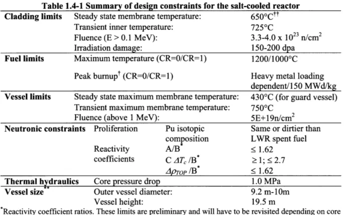
code for the materials employed. The salt reactor also uses the same metallic fuel as similar fast reactors, with the same temperature and burnup limits. In addition to materials constraints, there are reactor physics constraints relating to proliferation resistance and passive safety performance. These were found to be adequately met by reactor physics analyses and are not addressed in this report. Finally, there are a couple soft constraints which have a bearing on cost: the pressure drop across the core and the maximum vessel size. For pressure drop, a value of IMPa is used because it is comparable to that of existing fast reactors [IAEA, 2006], while for vessel size the dimensions of the lead-cooled FCR reactor & S-PRISM vessels are used for guidance. These constraints can be exceeded through the use of larger pumps or a larger vessel, although doing so would increase the capital cost of the salt system. A summary of the constraints adopted for this thesis is given in Table 1.4-1. More details regarding the development of constraints for FCR reactor systems are available in the NERI project quarterly reports.

(20)

Table 1.4-1 Summary of design constraints for the salt-cooled reactor Cladding limits Steady state membrane temperature: 650Ctt

Transient inner temperature: 7250C

Fluence (E > 0.1 MeV): 3.3-4.0 x 1023 n/cm2 Irradiation damage: 150-200 dpa

Fuel limits Maximum temperature (CR=0/CR= 1) 1200/10000_C

Peak burnupt (CR=0/CR=1) Heavy metal loading dependent/150 MWd/kg

Vessel limits Steady state maximum membrane temperature: 4300_{C (for guard vessel)}

Transient maximum membrane temperature: 7500C Fluence (above 1 MeV): 5E+19n/cm2

Neutronic constraints Proliferation Pu isotopic Same or dirtier than composition LWR spent fuel Reactivity A/B 1.62

coefficients C AT, /B* 2 1; <2.7 AdpToP /B* <_ 1.62

Thermal hydraulics Core pressure drop 1.0 MPa

Vessel size Outer vessel diameter: 9.2 m-10m

Vessel height: 19.5 m

*Reactivity coefficient ratios. These limits are preliminary and will have to be revisited depending on core temperatures

**S-PRISM (a non-pressurized vessel) dimensions taken as guidance

tAlloy-type fuel, taking into account cladding stress for given cladding dimensions and temperature limits, based on analyses in Hejzlar et al. [2004]

ttFor the CR=0 core, which has a content of Pu larger than 20wt%, a smaller limit than 6500_{C may be}

required, driven by fuel cladding chemical interaction (FCCI) issues since Pu may form an eutectic with iron resulting in cladding thinning. A large amount of Zr in the fertile free fuel will mitigate FCCI and the exact limit is currently uncertain. Also, a zirconium liner can be developed to prevent this eutectic

formation. The 6500C limit is consistent with the achievable category of materials, which were selected

for the analyses in the project and assume successful completion of ongoing R&D on materials development.

(21)

2. Methodology

2.1 Description of the subchannel model

A spreadsheet model mirroring the function of the SUBCHAN code [Todreas & Hejzlar, 2006b] was developed to quickly analyze different core geometries, operating conditions, and coolant salts. The SUBCHAN code was developed to design the lead-cooled FCR reactor; it analyses a core by dividing it into a number of non-communicating subchannels. Examples of the different types of subchannels in a square-lattice assembly are shown in Figure 2.1-1. Based on user-inputted core geometry, coolant inlet flow rate and temperature, and core power distribution, SUBCHAN calculates the core pressure drop, coolant outlet temperature, as well as maximum cladding and fuel temperatures.

--

t

1

P

-L

4

(22)

The spread sheet model developed similarly divides the triangular-array, wire-wrapped salt assemblies into non-communicating subchannels. "Non-communicating" means the assumption is made that there is no heat or mass transfer between the different subchannels. This

assumption is inaccurate for the salt core, because the presence of wire-wrap spacers leads to a great deal of mixing throughout each assembly. However, this assumption is conservative because mixing flattens the coolant temperature profile in each assembly, reducing the maximum

fuel and cladding temperatures, so a subchannel analysis is useful for providing quick and meaningful results. Each subchannel is divided into a number of axial meshes (one each for the reflector and shield regions below the core, 11 for the active core, and one for the gas plenums above the core). The channel geometries are specified, allowing the subchannel flow area (A) to be calculated. The peaking factor and axial flux shape of the subchannel are also specified, so the heat input to each subchannel mesh (Qi) can be computed. Given coolant inlet velocity (vo) and enthalpy (ho), conservation of energy (Equation 2.1-1) and mass (Equation 2.1-2) can be used to determine coolant velocity and enthalpy in subsequent axial nodes.

h

= h_, +

Q /

(2.1-1)

iPi = VoPo = m / A (2.1-2)

The subscript i designates the axial node number, and pi is the coolant density at node i, which along with coolant temperature, heat capacity, and thermal conductivity can be calculated from the coolant enthalpy hi.

With the coolant properties and flow velocity, correlations can be used to determine the friction factor and heat transfer coefficient for each subchannel mesh. For friction factor the Cheng-Todreas [1986] correlation is used, which was developed to deal specifically with wire-wrap

(23)

flow bundles. Very little work has been done on heat transfer in wire wrap bundles, especially for high Prandtl number fluids such as liquid salts. This is because the coolant commonly used in wire-wrapped bundles is liquid sodium, which has a low Prandtl number and yields very low film temperature rises, making the convective heat transfer coefficient less important. One study was performed by Fenech [1985] on wire-wrap heat transfer in water-cooled bundles, but his results were for a fixed geometry (P/D=1.05) and could not be directly applied. Therefore, an alternate approach was needed to model heat transfer in the liquid-salt cooled core.

The approach taken was to use the well known Gnielinski heat transfer correlation [1976], which applies to Re > 1000 for tube flow, and apply it to wire wrap flow. The Gnielinski correlation has the following form:

(Re-1000) Pr

Nu = Re>1000

1+ 127 _{1+ 12.7} _(Pr2/3 2 - 1)1) (1.82 log(Re) - 1.64)2 Re>1000 (2.1-3)

The Gnielinski correlation can be compared to the correlation developed by Fenech for a water cooled wire-wrap assembly (Eq. 2.1-4). This done by applying the Gnielinski correlation to the geometry tested by Fenech and setting the Prandtl number to 5.4, that of warm water. Results of the comparison are shown in Figure 2.1.-2.

Nu = h*DH - 1 0.0301 * Re 79

* Pr0.43 Re>2300

k Fhotspot (2.1-4)

h: heat transfer coefficient (W/m2_K)

DH: subchannel hydraulic diameter, including the wire (m)

k: coolant thermal conductivity (W/mK)

(24)

120 0I I I II I AI I I I 0 IA 20 --- - .--- - ... 0 2000 4000 6000 8000 10000 12000 14000 Reynolds number

Figure 2.1-2 Fenech and Gnielinski correlation comparison

Figure 2.1.-2 shows that the Gnielinski correlation yields smaller values for Nusselt number, with values about half those of the Fenech correlation near transition flow Reynolds numbers. This is likely evidence that there are heat transfer enhancement mechanisms caused by the wire-wrap geometry, such as enhanced flow turbulence. Such mechanisms would not be simple to model and would require additional experimental data to verify. Since the Gnielinski correlation

doesn't take these mechanisms into account, it should be considered a conservative estimate.

Also, it should be noted that the difference between the modified Gnielinski and Fenech correlations becomes more pronounced for Prandtl numbers in the liquid salt range (~30), with the Gnielinski correlation becoming even more conservative. Therefore, the heat transfer analysis in this report as a whole is very conservative, due to the use of both the non-communicating subchannel approximation and the Gnielinski correlation.

(25)

Given the friction factor at each node in a subchannel, the pressure loss across the entire subchannel is given by:

AP = . f i p.v + _ Pi-IVi21 )+-KL,i ip v (2.1-5)

S 2 1DH

2

Li: length of the ith mesh

DH: the subchannel's wetted hydraulic diameter (includes the wire perimeter) KL, : is any form loss (such as an orifice) associated with the ith mesh

The first term in the summation is the pressure loss due to friction, the second term is the pressure loss due to coolant acceleration (usually small), and the third term is the form loss.

Here the pressure change due to gravity has been neglected since it has relatively little effect on pumping power (there is a small natural circulation head present when the reactor is operating because of different density coolant in the chimney and downcomer). A form loss coefficient of

0.4 is introduced to the entrance and exit of the core bundle to represent flow contraction and expansion at these points. These form losses were introduced to mirror the original SUBCHAN input decks. While the value of 0.4 at the exit is smaller than the correct value of 1.0, the contribution of these form losses to the total core pressure drop is minimal so the actual values can be safely neglected.

Cladding temperatures are calculated by dividing the linear heat rate (Q i) at a mesh by the

thermal resistance (Ri) between the cladding and the coolant, and adding this temperature difference to the local coolant temperature:

(26)

1 In

Tcldi _cladicoolant,i _coolant2 / R ; + R + (2.1-6)

coh

i

2znkc

rco: cladding outer radius rc,: cladding inner radius

h,: local heat transfer coefficient (h, = k,*Nu/DH, where ki is the coolant thermal conductivity at

node i)

kc: cladding thermal conductivity

Here the temperature of the cladding's inner surface is used for comparison against the limit in

Table 1.4-1 since it is higher. Fuel temperatures are calculated in a similar way by adding terms

for the cladding inner oxide layer (roughly assumed to be 10 microns thick with a thermal

conductivity of 2W/mK), the lead-alloy fuel-cladding bond, and the fuel pin to the thermal

resistance. Note that SUBCHAN code uses node-averaged values for the linear heat rate, i.e. (Qi

+ Qi+1)/2 instead of Qi in Equation 2.1-6; this was changed for the spreadsheet model to better

match the calculations performed by RELAP. The method employed here yields maximum

cladding temperatures a few degrees higher than the SUBCHAN code.

Spreadsheet models were developed for interior, side, and corner subchannels of a hexagonal

assembly. The models can be used to calculate the coolant flow rates in each subchannel that

would produce a specified pressure loss. Coolant and cladding temperatures can also be

computed, which showed that interior channels generally have the highest cladding temperature.

Flow rate results for the subchannels can be summed to determine the total flow rate in an

assembly for a given pressure drop, which in turn allows the total flow rate in the core to be

(27)

assemblies) is neglected because it is assumed that these flow rates can be made arbitrarily small through orificing.

Benchmarking

The spreadsheet subchannel model is a recreation of the SUBCHAN code in a different format, and tests using lead reactor parameters showed that the two models' results agreed exactly. This is expected because the spreadsheet performs the same set of calculations that SUBCHAN does using the same fundamental equations. The only changes made to allow for salt reactor

modeling were the geometric parameters (square lattice to triangular), the correlations used, and the removal of node-averaged linear heat rates (see comments for Eq. 2.1-6). These changes were benchmarked by comparing the results to hand calculations (for the geometry changes) and the expected outputs for the correlations (from charts in the correlations' respective papers).

2.2 Orificing calculations

Without orificing, approximately the same coolant flow rate goes through each assembly. Orificing can be used to reduce coolant flow through the core, which is desirable because this raises the average outlet temperature, increasing plant efficiency. A reduced flow rate also reduces the pumping power required to move coolant through the core.

With the spreadsheet subchannel model, it is possible to quickly determine the minimum flow rate in an assembly, given its radial peaking factor and axial flux shape, which does not cause the

cladding temperature limit (6500C) to be exceeded. What results is an orificing map similar to that shown in Figure 2.2-2, corresponding to the assembly peaking factor map in Figure 2.2-1.

(28)

The numbers in the orificing map correspond to the relative flow rate in that assembly compared to the flow rate in the assembly with the maximum peaking factor (the hot assembly). Using the optimal orificing scheme shown in Figure 2.2-1, the flow rate in the core can be reduced about 23% from an unorificed core, a large improvement. However, the orificing scheme in Figure 2.2-2 uses a different orifice setting for nearly every assembly, and may be challenging to implement in practice. Another approach is to use the three-zone orificing scheme shown in Figure 2.2-3. This scheme minimizes the flow rate through the core using only three orifice

settings, producing a flow reduction of about 15%, yielding the majority of the benefit of the optimal scheme. Use of a three-zone orificing scheme raises the core outlet temperature from 5580_{C to 569}0_{C. The corresponding flow rate, 85% of the unorificed value, was subsequently}

assumed for calculating core performance parameters.

0 1 2 3 4 5 6 7 8 9 10 11 12 0.59 5 1.08 0.85 0.58 4 1.17 1.24 1.01 0.83 0.55 3 1.18 1.21 1.16 1.21 1.03 0.78 0.50 > 1.26 1.24 1.20 1.07 1.16 0.91 0.70 0.43 L 1.26 1.23 1.17 1.08 1.09 0.87 0.59 ) 1.25 1.14 1.13 0.97 1.00 0.75 0.47 L 1.26 1.23 1.17 1.08 1.09 0.87 0.60 2 1.26 1.24 1.20 1.07 1.16 0.91 0.70 0.43 3 1.18 1.21 1.16 1.21 1.03 0.78 0.50 1.17 1.24 1.02 0.83 0.55 5 1.08 0.85 0.58 S0.59

(29)

0 1 2 3 4 5 6 7 8 9 10 11 12 10.419 1.000 1.000 0.990 I0.922 0.951 I0.912 Figure 2.2-2 0.970 0.941 0.903 0.981 0.828 CR=1 0.922 0.980 0.970 0.883 0.912 0.818 0.951 0.774 0.628 orificing 0.951 0.941 0.912 0.873 0.827 0.903 0.783 0.611 0.411 0.912 0.903 0.818 0.827 0.729 0.837 0.678 0.570 0.388 0.981 0.951 0.903 0.837 0.828 0.765 0.783 0.678 0.645 0.756 0.545 0.628 0.611 0.570 0.505 0.419 0.329 0.411 0.388 0.351 0.300 0.645 0.427 0.505 0.300 0.351

flow rate map

0 1 2 3 4 5 6 7 8 9 10 11 12 0.427 0.427 0.427 0.427 0.427 0.427

0.427

0.27 .4277

Figure 2.2-3 CR=1 Three-zone orificing flow rate map

The values in Figures 2.2-1 through 2.2-3 are just for the core beginning-of-life power map; the power map changes somewhat over the life of the core. Similar orificing calculations can be performed for middle-of-life and end-of-life power maps, yielding two more flow rate maps similar to Figure 2.2-2. Another flow rate map can be constructed using the maximum values for each assembly position from the BOL, MOL, and EOL maps, which would represent the ideal

(30)

fixed orifices for the life of the core. At the time orificing calculations were performed for the salt reference cores, MOL and EOL data were not available, so their contribution to the overall orificing picture was not included. However, when performing the same study for the lead FCR reactor, it was found that because the radial flux shape changes little over the life of the core, this effect amounts to less than a 3% increase in coolant flow rate. Given the already large

uncertainties in heat transfer calculations for the salt reactor this small factor was neglected.

Subchannel and orificing calculations were also performed for the CR=O salt core, which found that despite needing a higher coolant flow rate through the hot assembly (due to higher peaking), the CR=O core is more amenable to orificing, allowing the total core flow rate to be lower than that of the CR=1 core. Since the FCR reactor is designed to operate with both cores

interchangeably, the higher CR=1 core flow rate was assumed for the CR=O core as well. Power peaking and flow maps for the CR=0O case are given in Figures 2.2-4 through 2.2-6.

0 1 2 3 4 5 6 7 8 9 10 11 12 0.90 1.35 1.17 0.89 1.15 1.13 1.06 1.14 0.86 1.12 0.93 0.93 1.11 1.03 1.09 0.80 0.90 0.92 1.14 1.13 0.89 1.00 1.03 0.72 1.11 1 0.92 0.93 1.12 1.07 1.20 0.93 0.91 1.13 0.92 0.90 1.31 1.09 0.78 1.11 0.92 0.93 1.12 1.08 1.20 0.93 0.90 0.92 1.14 1.14 0.89 1.00 1.03 0.72 1.13 0.93 0.93 1.12 1.03 1.09 0.80 1.15 1.13 1.06 1.14 0.86 1.35 1.17 0.89 S0.90

(31)

0 1 2 3 4 5 6 7 8 9 10 11 12 FO . 6217 0.824 0.613 0.590 0.544 1.000 0.807 0.748 0.841 0.815 ____ 6~ 4 I t I 0.798 0.645 0.645 0.790 0.725 0.773 0.621 0.637 0.815 0.807 0.613 0.701 0.725 10.484 0.790 0.637 0.645 0.798 0.757 0.866 0.645 0.629 0.807 0.637 0.621 0.964 0.773 0.529 0.637 0.645 0.798 0.765 0.63 0 64 I 0.815 0.815 0.613 0.701 0.866 0.725 0. 8 I 0 6

I0.807

0.645 0.645 0.798 0.725 0.773 SI * 4 I I 0.807 1.000 0.748 0.815 0.841 0.613 0.590 0.544 0.645 0.484 0.621

CR=0 orificing flow rate map

0 1 2 3 4 5 6 7 8 9 10 11 12 0.645 0.645 0.645 0.645 0.645 0.645 0.645 0.645 0.645 0.645 F 0.645 _i

Figure 2.2-6 CR=O Three-zone orificing flow rate map

2.3 Description of RELAP model

RELAP5-3D/ATHENA is a code developed at Idaho National Laboratory for the simulation of thermal hydraulic systems [RELAP, 2005], and is referred to interchangeably as "RELAP" in this thesis. A RELAP model was constructed of the salt reactor system, including the primary

S0.824

Figure 2.2-5

(32)

coolant loop, power conversion system, ultimate heat sink, and auxiliary heat removal systems. This model is able to simulate the salt reactor's behavior for different steady state configurations and transient scenarios. The RELAP model for the salt reactor was constructed based on the RELAP model for the similarly configured lead-cooled FCR reactor, which itself was based on an earlier lead-bismuth reactor model developed at INL. RELAP model development for the salt reactor was performed in several stages:

1. Properties of the selected coolant salt were implemented in RELAP

2. A separate core model was created based on results from the spreadsheet subchannel analysis to yield the correct core average and limiting behavior.

3. A model of the intermediate heat exchangers was created based on results from a previously developed heat exchanger spreadsheet model.

4. Core and IHX component models were benchmarked and incorporated into a complete system model including the power conversion system and auxiliary heat removal systems.

5. The power conversion system's precooler sizes were adjusted slightly to yield the

correct steady state system temperatures.

6. Lithium expansion module (LEM) and passive secondary auxiliary cooling system (PSACS) designs were finalized based on transient simulation results.

Salt implementation

The ternary chloride salt NaCl-KCl-MgCl2 (30%-20%-50%) was selected based on neutronic and subchannel analyses as described in the salt selection section of this thesis. It was necessary

(33)

to first implement the properties of the selected coolant salt into the RELAP5-3D executable before any of the salt systems could be modeled. This was done by Cliff Davis at Idaho National Laboratory and Matthew Memmott at MIT, based on the set of salt properties submitted to them for this thesis. In addition to the basic thermal hydraulic properties described in the salt

properties section (density, viscosity, thermal conductivity, and heat capacity), RELAP also requires values for salt isothermal compressibility, vapor pressure, vapor properties, surface tension, as well as triple point and critical point properties. Data for many of these properties do not exist, so values similar to properties of other liquid salts were used. Since the coolant in the

liquid-salt cooled reactor never approaches the saturation line or sonic velocities, the values of these properties have no effect on the results obtained. The salt property values implemented into RELAP are given in Tables 2.3-1 numbers 1 through 9 below. The symbols for the properties are the same as those used in the report "Implementation of Molten Salt Properties into RELAP5-3D/ATHENA" (INEEL/EXT-05-02658).

Tables 2.3-1 NaCl-KCl-MgCl 2 (30%-20%-50%) properties for RELAP

Table 1. Constants for liquid salt

Tmelt (K) 669.15 AD (kg/m -K) -0.778 BD (kg/m3) 2260 A, (1/Pa) 1.62E-10 BK (1/K) 0.0018 cp (J/kg-K) 1005.

Table 2. Parameters for vapor components

Component Mi (g/mol) Cpi (J/mol-K)

NaCl 58.443 37.921

KCl 74.551 38.061

(34)

Table 3. Constants for salt vapor

M (g/mole) 80.049

R (J/kg-K) 103.862

Cp (J/kg-K) 662.9

Table 4. Saturation line constants

Asat 8.806

Bsat (K) 10375

Table 5. Values for triple and critical points

To (K) 669.15

Po (Pa) 2.668E-5

Tcrit (K) 2615.1

Pcrit (Pa) 9.196E6

Table 6. Reference values for specific internal energy and specific entropy.

ufo (J/kg) 0.0 sfo (J/kg-K) 0.0 ugo (J/kg) 8.164E5 sgo (J/kg-K) 3201 ucrit (J/kg) 1.9042E6 scrit (J/kg-K) 1356

Table 7. Constants for transport properties of liquid.

A, (Pa-s)

1

5.18E-5

B (K) 3040

K (W/m-K) 0.39

Table 8. Constants for surface tension.

A_o(N/m-K) -4.31E-5

B, (N/m) 0.1131

Table 9. Parameters used for calculating the dynamic viscosity of the vapor components.

Component Mi (g/mol) i Tmelt (K) V e

(J/mole-K) (cm3/mole) (Ki (A)

NaCl 58.443 37.921 1073.8 35.68 2062 4.02

KCl 74.551 38.061 1044.0 46.38 2004 4.39

MgC1₂ 95.211 61.748 987.0 53.84 1895 4.61

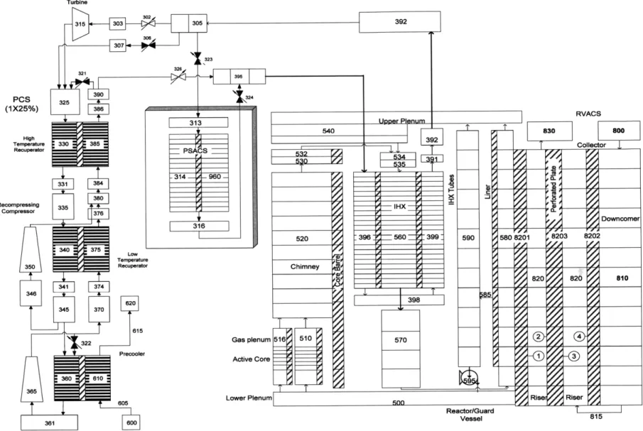
Overview ofRELAP nodalization

The nodalization diagram created for the lead-cooled FCR reactor [Todreas & Hejzlar, 2008b] is shown in Figure 2.3-1. The salt reactor model nodalization is identical in nearly every respect, aside from some differences explained in the subsection about virtual free levels. The volumes

(35)

numbered in the 500s correspond to the liquid salt primary system, the 100s, 200s, 300s, and 400s make up the four CO2 secondary trains, 600s to the ultimate heat sink water, 800s to the RVACS air, and 900s to the PSACS water tanks. Time-dependent volumes (effectively infinite mass sources/sinks) are set up to represent the boundary conditions for the open RVACS and ultimate cooling systems, as well as to represent a virtual "atmosphere" for the primary circuit.

(36)

Turbine PCS (1X25%) High Temperature Recuperator Recompressing Compressor Low Temperature Recuperator Gas plenum RVACS Active Core ' -605

605 Lower Plenum r Rise /A Riser

Reactor/Guard

Vessel 815

(37)

Beginning at the lower plenum below the core, volume 500, coolant moves through volumes 510 and 516 which represent the core. Volume 516 is the hot channel and volume 510 is the average channel; together they model both the overall performance of the core as well as its performance in the most limiting assemblies. Each core volume is divided into 23 axial nodes, one each for the reflector and shield below the core, 11 for the active core, and 10 for the gas plenums above the core. Above the core is volume 520, the chimney, which in the salt reactor is bottlenecked to allow more room for the intermediate heat exchangers. Volumes 530 through 540 are at the top of the reactor vessel and distribute coolant from the chimney to the annulus above the four intermediate heat exchangers, volume 560 through 563. The set of downcomers below the heat exchangers is volume 570, which connects to volume 580, the peripheral riser. The riser is connected to volume 590, the second set of downcomers, then the reactor coolant pump, volume

595, pumps coolant back into the lower plenum.

The remaining systems (RVACS air and power conversion system) are taken from the lead-cooled FCR reactor model and were not appreciably modified during this project, other than to

connect them appropriately to the liquid salt primary system. One exception is the design of the PSACS, which was changed in the course of transient analysis; these changes are described below in the PSACS modeling subsection and later in the transient analysis section.

RELAP core model

As described above, the salt core is divided into a hot channel and an average channel. Each channel is axially divided into 23 regions, one each for the blanket and reflector, 11 for the heated region of the core, and 10 for the gas plenum/LEM region above the core. Since the

(38)

interior subchannels of the hot assemblies have the highest cladding temperatures, the hot channel in the RELAP model is composed exclusively of interior subchannels, rather than of entire assemblies. This hot channel is equivalent to the heated interior subchannels of 12 assemblies, all using a hot subchannel peaking factor 2% greater than the highest assembly peaking factor, the same peaking factor used in the subchannel model.

A summary of the core RELAP implementation is given in Tables 2.3-1 and 2.3-2. The hot channel area is different for the two conversion ratios because the CR=1 core has more fuel rods and thus more heated channels per assembly. Because of higher peaking in the CR=0 core, the average channel is more strongly orificed, directing more flow through the hot channel. For the power multipliers, values are listed starting from the bottom of the core. Fuel conductivities for the salt reactor cores are given in Table 2.3-3.

Table 2.3-1 Orificing and flow split in the core

CR=1 CR=0

Highest assembly peaking factor 1.26 1.35

Number of assemblies 12 12

Channel area (m2

) (hot/average) 0.09391/4.48985 0.09224/4.49152 Orificing coefficients (hot/average) 0.0/13.610 0.0/23.116 Mass flow rate (kg/s) (hot/average) 771./ 32034. 833./ 31972.

Table 2.3-2 Internal power multipliers.

CR=1 CR=0

Relative Average Hot Relative Average Hot

0.706 0.06218 0.00199 0.601 0.05282 0.00182 0.886 0.07804 0.00250 0.823 0.07233 0.00249 1.057 0.09310 0.00299 1.014 0.08912 0.00306 1.187 0.10455 0.00335 1.158 0.10177 0.00350 1.261 0.11106 0.00356 1.247 0.10960 0.00377 1.276 0.11239 0.00360 1.277 0.11223 0.00386 1.229 0.10825 0.00347 1.246 0.10951 0.00376 1.124 0.09900 0.00317 1.157 0.10169 0.00350 0.966 0.08508 0.00273 1.016 0.08929 0.00307 0.766 0.06747 0.00216 0.832 0.07312 0.00251 0.543 0.04783 0.00153 0.629 0.05528 0.00190

(39)

Table 2.3-3 Fuel conductivities (W/mK) Temperature (K) CR= 0 CR= 1 293 3.75 8.22 373 4.60 9.00 873 10.95 15.26 1173 13.70 20.14 1873 22.80 34.81

A simplification is made for modeling wire-wrap pressure drop in the salt core by adapting RELAP's Colebrook & White correlation to match the results given by the Cheng-Todreas correlation. This was done by varying the value of the surface roughness parameter in the Colebrook & White correlation so that the total pressure drop across the hot channel matched that in the subchannel model. Compared to the Cheng-Todreas correlation, this adapted Colebrook & White correlation has a weaker dependence on Reynold's number; it tends to underpredict the friction factor for lower Reynolds numbers and overpredict it for higher Reynolds numbers. Over the range of Reynolds numbers for the reference core at steady state, the relative error is less than 5%, which is less than the uncertainty of each correlation. This simplification may affect the accuracy of modeling transient behavior, which involves low Reynolds numbers, but is needed because RELAP does not include an implementation of the Cheng-Todreas correlation.

To benchmark the RELAP core model, it was run at 2400 MWt and a total coolant flow rate of 3.28E4 kg/s, corresponding to the nominal steady state operating conditions. The pressure drop across the core and coolant and cladding temperatures were compared to the values obtained by the subchannel model. Results are given in Figures 2.3-2 and 2.3-3. As these figures show, there is extremely good agreement between the RELAP model developed and the subchannel model used to develop the core. The total pressure drop across the core matches within 2 kPa,

(40)

the matching coolant temperatures show the correct flow split has been achieved, and the peak cladding temperature matches within 1 'C.

1.4E+06 1.2E+06 1.0ES06 oubchan 1o 0> 0 0, 1 x RELAP O : O o 6.0E+05 4.0E+05 2.0E+05 0.0E+00 0 0.65 1.3 1.95 2.6 3.25 3.9 Axial position (m)

Figure 2.3-2 RELAP and subchannel model pressure drop comparison

700

650

o Subchan avcore coolant R

a Subchan hotchan coolant

S600 o Subchan max clad x RELAP avcore coolant

x RELAP hotchan coolant

x RELAP max clad a ,

550 -I- ® 500 'a 450 0 0.65 1.3 1.95 2.6 3.25 3.9 Axial position (m)

(41)

Lithium expansion module model

The hydrodynamic volumes and heat structures above the core corresponding to the gas plenums are structured to incorporate the presence of LEMs. They are divided into 10 axial nodes, each 0.13 meters long, to obtain a better estimate of time dependent heat transfer to the LEMs. A heat structure representing the LEM lithium reservoirs are present above the core average channel, alongside the heat structure for the gas plenums. These LEM heat structures consist of three radial nodes bounding two meshes: the first mesh extends from a radius of 0.0mm to 3.26mm and is composed of liquid lithium, and the second mesh extends from 3.26mm to 3.76mm and is composed of T-91 cladding material. Heat transfer in the liquid lithium is assumed to be due to conduction only, which is reasonable for liquid metals. Molten lithium properties are taken from Ohse, 1985. Heat transfer from the primary coolant to the LEMs is calculated using the same Gnielinski correlation used for the active core.

The average temperature of the liquid lithium at the centerline node of the LEM heat structure is calculated using RELAP control variables. This LEM reservoir temperature is converted to a reactivity insertion using a RELAP general table function, according to the

temperature-reactivity curves specified in the section on lithium expansion module design, and is added to the contributions from the other reactivity feedbacks. The reactivity contribution of LEMs is also given in the reactivity parameter implementation subsection of this section.

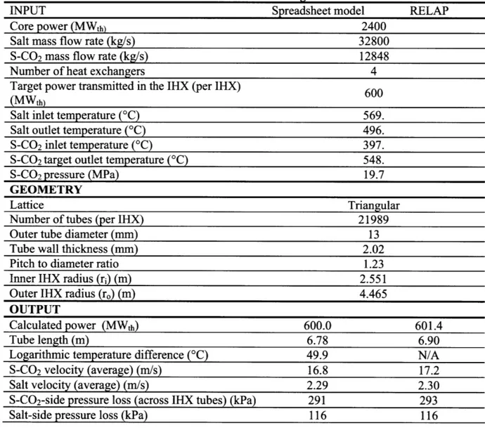
Intermediate heat exchanger model

The salt reactor intermediate heat exchangers were designed using the spreadsheet model developed by Anna Nikiforova to design the lead reactor IHXs, with the primary side heat transfer correlation changed to the Gnielinski correlation, which is appropriate for high Prandtl

(42)

number liquid salts. A comparison of RELAP model results with the spreadsheet results is given in Table 2.3-4. The two sets of results do not match exactly because RELAP uses a slightly different correlation (Colebrook-White with fitted roughness term instead of McAdams) for pressure losses than the spreadsheet model. Also, the RELAP model incorporates the power lost

through the RVACS and power gained from the reactor coolant pumps, meaning the RELAP heat exchangers do not reject exactly 600MW each. Nevertheless, results agree very well and validate the performance of the RELAP model.

Table 2.3-4 Comparison of spreadsheet and RELAP model results for the salt reactor intermediate heat exchangers

INPUT Spreadsheet model RELAP

Core power (MWth) 2400

Salt mass flow rate (kg/s) 32800

S-CO2 mass flow rate (kg/s) 12848

Number of heat exchangers 4

Target power transmitted in the IHX (per IHX) 600

(MWth)

Salt inlet temperature (oC) 569.

Salt outlet temperature (oC) 496.

S-CO2 inlet temperature (oC) 397.

S-CO2 target outlet temperature (°C) 548.

S-CO2 pressure (MPa) 19.7

GEOMETRY

Lattice Triangular

Number of tubes (per IHX) 21989

Outer tube diameter (mm) 13

Tube wall thickness (mm) 2.02

Pitch to diameter ratio 1.23

Inner IHX radius (ri) (m) 2.551

Outer IHX radius (ro) (m) 4.465

OUTPUT

Calculated power (MWth) 600.0 601.4

Tube length (m) 6.78 6.90

Logarithmic temperature difference (OC) 49.9 N/A

S-CO2 velocity (average) (m/s) 16.8 17.2

Salt velocity (average) (m/s) 2.29 2.30

S-CO2-side pressure loss (across IHX tubes) (kPa) 291 293

(43)

Virtual free level model

A limitation in the current RELAP5-3D version prevents the modeling of free levels for some coolants, including sodium and liquid salt. This limitation relates to partial pressure of coolant vapor in the gas-filled free space. Thus, the primary system model cannot include any air and must be completely filled with coolant. However, free levels are an integral part of the dual-free-level design, and free dual-free-level positions must be known to determine if there is any overflow or if any components become exposed to air. Furthermore, the free level position in the outer annulus determines the amount of heat removed by the RVACS, since heat transfer to the guard vessel is much higher below the free level than above it. To account for free level positions without being able to explicitly model them, "virtual free levels" were built into the salt reactor RELAP model.

To construct the virtual free level model, first, volumes where air would have been present in the reactor vessel are removed from the model (parts of volumes 540 and 580, as well as all of volume 599). This way, the virtual free level model can contain the same amount of coolant and have the same thermal inertia as the actual reactor system. What results are two "ceilings" close to where the free levels should be, one above the chimney and one along the periphery of vessel, where the second riser and downcomer are. This is depicted in Figure 2.3-4, with the dot-dash lines indicating the positions of the ceilings.

(44)

Time dependent volume I I I I--I I --- I

Figure 2.3-4 Vessel layout showing virtual free levels and time dependent volume

In order to allow for thermal expansion, a time-dependent volume (number 588) was connected to the top of peripheral riser; this functions similarly to a pressurizer by holding the pressure constant while allowing coolant to enter and exit. With this model, it is possible to calculate where the free level positions should be based on the pressures at the ceilings and total mass of coolant in the system. First, imagine that the "correct" free level positions exist at height ha and

(45)

hb above the ceilings, where the subscript a denotes the hot free level (chimney) and b denotes

the cold free level (periphery); these heights can also be negative. Then, the total mass of coolant in the system is given by:

Mtotal = Mmodel,i + Pa,iAaha,i + Pb,iAbhb,i = Mmodel + PaAaha + PbAbhb (2.3-1)

Here A is the area of the free level, p is the coolant density at the free level, and the subscript i

represents initial or nominal conditions. Mmodel is the total mass of coolant modeled by RELAP,

the actual total coolant mass Mtotal is equal to this mass plus the mass of the "virtual" coolant not

modeled (Recall that vessel volume is initially chosen so that Mtota Mmodel,i). This equation

takes into account the effect of thermal expansion; if the coolant heats up and expands, some of it

will be pushed into the time-dependent volume, reducing the mass of coolant in the model. For

the total coolant mass to remain constant, there must be more virtual coolant, i.e. the free levels

must rise. To determine the relative position of the free levels, one can use the fact that both free

levels are at the same atmospheric pressure:

Pa -p gh, = P - pghb Ptm (2.3-2)

Here Pa and Pb are the coolant pressures measured by RELAP at the "ceilings" of the model;

subtracting the hydrostatic pressure due to virtual coolant yields the pressure at the virtual free

levels. Together these two equations allow one to solve for the free level positions ha and hb,

since all other quantities can be derived from RELAP output.

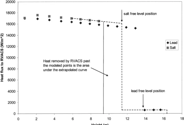
The final component of the virtual free level model is connecting the position of the peripheral

(46)

from the atmosphere above the coolant free level is much lower than from the coolant below the free level. This is done using a first-order approximation, depicted graphically in Figure 2.3-5.

The diamonds show RVACS heat flux as a function of height along the periphery in the lead-cooled FCR reactor model, which uses an explicitly modeled free level. One can see that the heat flux decreases linearly below the free level, then falls dramatically to an approximately

constant value above the free level, where heat transfer from the air inside the vessel to the guard vessel constitutes the primary thermal resistance. One can assume similar behavior exists for the

salt reactor - a linear decrease below the free level then a small and constant value above it. In the virtual free level salt reactor model, only heat fluxes below the ceiling are computed by

RELAP, however these heat flux values for the salt reactor can be extrapolated to the virtual free level position as shown by the dashed line in Figure 2.3-5. Above the free level the heat flux is assumed to have the same constant value as for the lead reactor, which is reasonable since the air in the salt and lead reactor vessels will be similar. The total heat removed by the RVACS is then the sum over the modeled heat fluxes and the extrapolated amount, which is the L-shaped area under the dashed curve in Figure 2.3-5. Control variables are used to perform the extrapolation

described and calculate the total amount of additional heat that should be removed by the RVACS. To actually remove the heat from the coolant in the virtual free level model, an artificial heat structure is set up at the top of the peripheral riser that rejects the amount of heat calculated by these control variables.

(47)

20000

18000 salt free level position

16000*

oi 14000

{E _Lead

12000 USalt

10000

-o Heat removed by RVACS past

the modeled points is the area

5 8000 _{under the extrapolated curve}

i 6000

4000- lead free level position

2000

1

L..---- -- •--l

0-I

0 2 4 6 8 10 12 14 16 18

Height (m)

Figure 2.3-5 RVACS heat flux as a function of position

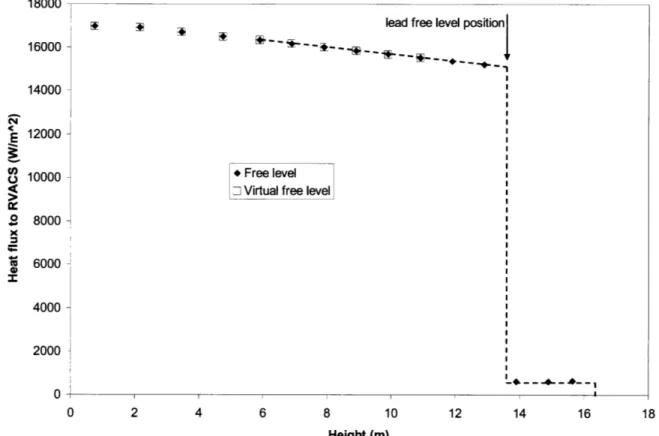
To benchmark the virtual free level model, it was implemented in the lead-cooled reactor RELAP model and results from this model were compared to those of the original model. The testing demonstrated that heat fluxes from the coolant to the RVACS were nearly identical for the virtual free level model and the original (explicit free level) model, (Figure 2.3-6) showing that the linear extrapolation method employed is accurate. While the virtual free level model possesses the same thermal inertia as the system being modeled, it does not account for the movement of coolant masses. For example, during a loss of flow accident the coolant level will fall in the chimney and rise in the periphery; in the virtual free level model this movement is tracked but no actual coolant migration occurs. Finally, there is a small error introduced by the movement of coolant into and out of the time dependent volume due to thermal expansion; this

(48)

amount is less than 5% for a bounding accident and therefore does not significantly impact results.

18000

1 W lead free level position

16000 --- - -

-14000

E 12000

S10000 Free level

7 Virtual free level

8000 W 6000 4000 2000 0 i 0 2 4 6 8 10 12 14 16 18 Height (m)

Figure 2.3-6 RVACS heat flux for explicit- and virtual-free-level models

PSA CS modeling

The Passive Secondary Auxiliary Cooling System (PSACS) is a novel decay heat removal

system designed for the lead-cooled flexible conversion ratio reactor [Todreas & Hejzlar, 2008b]. The PSACS consists of an passive auxiliary heat exchanger (PAHX) connected to each power conversion system train via valves, which can discharge heat into large water tanks during transients. Adjusting the design of the PAHX and size of the PSACS water tanks has a large

(49)

The original dimensions for the lead FCR reactor PSACS are given in Table 2.3-5. Because the salt PSACS designs were derived from this original lead design, the different iterations are named based on the relative power removed by the PSACS system and the capacity of the

PSACS water tanks. The different motivations for resizing the PSACS for the salt system are explained in the transient analysis section.

Table 2.3-5 Salt reactor PSACS design iterations*

Design iteration Original Previous Reference

lead design salt design salt design

Design designation 200% power, 100% power, 60% power,

1.0x tank size 1.1x tank size 0.75x tank size

Water Tank Height (m) 12.0 -13.2 -9.0

Diameter (m 6.0 -6.0 -6.0

Passive Number of tubes 700 -500 -350

Auxiliary Tube length (m) 4.0 -3.0 -2.4

Heat Inner diameter - 8.00E-03 8.00E-03 8.00E-03

Exchanger CO2 side (m)

(PAHX) Tube thickness 2.80E-03 2.80E-03 2.80E-03

(m)

Outer diameter - 1.36E-02 1.36E-02 1.36E-02

water side (m)

P/D ratio 3 3 3

*Parameters for the salt designs are estimates; see simplifications below

The original lead PSACS design was modeled explicitly in RELAP as hydrodynamic volumes and heat structures with the geometry given in Table 2.3-5. Two simplifications were used to model the subsequent PSACS designs. First, RELAP code runs stall when the PSACS tanks are nearing depletion; so it was necessary to introduce a PSACS trip (closure of the PSACS valves) shortly before this occurs in order for RELAP runs to proceed past this point. To simplify the modeling process, the PSACS tanks were made arbitrarily large in the model so the code would not stall, and the PSACS trip time was set to the desired time for the PSACS to run out of water.

(50)

The physical size of the PSACS tanks could then be calculated from the amount of energy removed by the PSACS system while it was operating.

The second simplification employed has to do with modeling of the PAHXs. Different sized PAHXs were modeled by first removing a train from the original PSACS design and then by adjusting the heat structure length parameter of the PAHX heat structures. Removing one of the two operating trains, rather than downsizing each train by 50%, was necessary because RELAP

encounters computation difficulties modeling individual low power PSACS trains. The resulting single train in the model functions equivalently to two half-sized PSACS trains. Changing the heat structure length in the PAHX heat structures is a convenient way of scaling the overall

PSACS power capacity. Decreasing the heat structure length parameter corresponds physically to either reducing the heat transfer area or increasing the thermal resistance of the PAHX tubes,

and has no effect on pressure losses in the system. In an actual system, downsizing of the PAHXs would be likely to occur via reducing the number and length of the PAHX tubes, which is reflected in Table 2.3-5. Since use of the above two simplifications allows one to avoid explicitly modeling both PSACS water tank and PAHX geometries, the values given for the salt designs in Table 2.3-5 are given as estimates.

2.4 Salt reactor reactivity feedback implementation

In addition to steady state simulations of reactor performance, RELAP5-3D is also able to perform transient simulations using inputted reactivity data. For the purposes of RELAP modeling, beginning of life (BOL) reactivity data are used because they are more challenging in terms of transient response. Reactivity calculations were performed by Eugene Shwageraus, a