HAL Id: hal-01226760
https://hal.inria.fr/hal-01226760v3
Submitted on 2 Aug 2016
HAL is a multi-disciplinary open access
archive for the deposit and dissemination of
sci-entific research documents, whether they are
pub-lished or not. The documents may come from
teaching and research institutions in France or
abroad, or from public or private research centers.
L’archive ouverte pluridisciplinaire HAL, est
destinée au dépôt et à la diffusion de documents
scientifiques de niveau recherche, publiés ou non,
émanant des établissements d’enseignement et de
recherche français ou étrangers, des laboratoires
publics ou privés.
Using counters for absence prediction in Esterel
Bernard Paul Serpette
To cite this version:
Bernard Paul Serpette. Using counters for absence prediction in Esterel. [Research Report] RR-8941,
INRIA Sophia Antipolis - Méditerranée. 2016, pp.18. �hal-01226760v3�
0249-6399 ISRN INRIA/RR--8941--FR+ENG
RESEARCH
REPORT
N° 8941
Août 2016absence prediction in
Esterel
Bernard P. Serpette
RESEARCH CENTRE
SOPHIA ANTIPOLIS – MÉDITERRANÉE
Bernard P. Serpette
Project-Team Indes
Research Report n° 8941 — Aoˆut 2016 — 18 pages
Abstract: Esterel is a synchronous programming language historically defined for system control, well suited to react in parallel to external sensors, intensively used in avionics. Recently, with the incoming of the orchestration language HipHop, a domain-specific language of the multi-tier language Hop, Esterel is used to manage Web requests. In this context, where orchestration programs are dynamically generated, long compilation preamble to computation must be avoided and a simple and fast interpreter is preferred. This paper presents such an interpreter. Esterel’s processes communicates through signals and one particularity of this language is its ability to instantaneously react to the absence of a signal. In this paper we present a static analysis which allows the interpreter to predict the absence of a signal.
Key-words: synchronous languages, instantaneous reaction to absence, interpretation, contin-uations, formal proof
Utilisation de compteurs pour la pr´
ediction de l’absence en
Esterel
R´esum´e : Esterel est un langage synchrone historiquement d´efini pour les syst`emes de contrˆole, parti-culi`erement adapt´e pour r´eagir en parall`ele `a des ´ev`enements externes, utilis´e intensivement dans l’avionique. R´ecemment, avec l’arriv´ee du langage d’orchestration HipHop, un sous-langage d´edi´e de Hop, l’approche Es-terel est utilis´ee pour synchroniser des requˆetes Web. Dans ce contexte, o`u les programmes d’orchestration sont g´en´er´es dynamiquement, les longs pr´eambules de compilation sont `a ´eviter et l’utilisation d’interpr`etes simples et rapides devient souhaitable. Cet article pr´esente un tel interpr`ete. Les processus Esterel commu-niquent au travers de signaux et l’une des particularit´es de ce langage est sa capacit´e de r´eagir instantan´ement `
a l’absence d’un signal. Dans cet article, nous pr´esentons une analyse statique qui permet `a l’interpr`ete de pr´edire l’absence d’un signal.
Mots-cl´es : langages synchrones, r´eaction imm´ediate `a l’absence, interpr´etation, continuation, preuve formelle
1
Introduction
We informally present the Esterel programming lan-guage focusing on the notion of process. An Esterel program is made of several processes, each of them executing statements. The processes communicate via signals. A process can raise a signal S with the statement ”emit S”. Once emitted, a signal is visible by all the processes. Signals can be tested with the statement ”present S then P1 else P2 end”. If the
signal S is already emitted, the evaluation continues with P1. We will detail this statement latter in this
section. A process can emit a signal but cannot reset it, as if it was never been emitted. The only way to reset a signal is to erase all signals at the same time defining a notion of instant. All processes must coop-erate to reach the end of one instant. Individually, a process may decide to finish its instant by executing the statement ”pause”, and it is when all processes have executed a pause or have finished their execu-tion that the current instant is globally closed.
Processes are generated via a statement ”P1kP2”.
At runtime two processes are created, one executing P1, the other executing P2, the main process waiting
for the completion of its two sub-processes before con-tinuing its own execution. The execution of P1 and
P2may take several instants. The two sub-processes
must join on completion before resuming the execu-tion of their creator.
Coming back to the ”present” statement, if one process have to evaluate a statement ”present S then P1else P2end”, the signal S may
be in an undefined state : not yet emitted but a con-current process having the opportunity to emit it. In this case, the current process will wait until the sta-tus of the signal is defined. A signal is present once an ”emit ” is evaluated. Conversely, a signal is ab-sent if and only if it is not emitted in the instant. So, to predict the absence of a signal in a middle of an instant, we have to look in the future to prove that no process will emit it. In this work, to detect the absence of a signal, we maintain a prediction of how many times a signal may be emitted by all processes until the end of the current instant. The prediction is correct if, when the count of a signal reaches zero, then the signal cannot be emitted during the instant.
The prediction is over-estimated. If for a signal the prediction gives a value of n, this means that, for the rest of the instant, the signal can be emitted at most n times. For a ”present” statement, both the ”then”and the ”else” part of the statement are con-sidered as reachable when predicting. Dynamically, when one branch of control will be taken, the poten-tially emitted signals of the other branch is erased from the prediction.
Let’s consider a simple example (”P1;P2” is the
sequence of the two statements P1and P2) :
(P; emit S)
|| present S then emit Y else emit N end If the statement P is a ”pause”, then ”emit S” will be done in the next instant and the count associated to S is zero; thus, the signal can be considered as absent and the signal N is emit-ted. If the statement P is ”nothing” (a state-ment that does nothing, runs in no time without emitting any signal), the count associated to S is one and the signals S and Y will be emitted. Fi-nally, consider the case where the statement P is ”present I then pause else nothing end”; stati-cally we cannot know if ”emit S” will be executed in the current instant or in the next instant; in this case the prediction for S is one, but dynamically, if the signal I becomes present, the count for S is decre-mented by one, reaching the value 0, and the signal S can safely be considered as absent.
In this paper we define a static analysis that creates these predictions and attaches them to programs. We also describe how an interpreter uses this information to predict the absence of signals. Finally, we prove that signals predicted absent are not emitted during the instant.
The rest of the paper is organised as follows. Sec-tion 2 finishes to introduce informally the semantics of Esterel. Section 3 defines the static analysis which associates to the nodes of the abstract syntax the pre-diction of how many times each signal can be emit-ted. Section 4 defines the interpretation of the dec-orated nodes and how the predictions are used and dynamically updated. In this section, we also discuss on continuations which implies trampolines
techno-Using counters for absence prediction in Esterel 4
nothing N op N op
pause P ause P ause+(σ)
emit S Emit(S) Emit(S)
P1;P2 Seq(P1, P2) Seq(P1, P2)
P1kP2 P ar(P1, P2) P ar+(P1, P2, σ)
present S then P1 else P2end If (S, P1, P2) If+(S, P1, σ1, P2, σ2)
loop P end Loop(P ) Loop+(P, σ)
trap T in P end T rap(T, P ) T rap+(T, P, σ)
exit T Exit(T ) Exit(T )
signal S in P end Signal(S, P ) Signal+(S, P, n) Figure 1: Syntax, AST and decorated AST of core Esterel
logy, show the synchronisation reclaimed by the par-allelism operator, and present some implementations of the waiting processes. In Section 5 we formally describe the analysis and the evaluator expressed in the Coq1 system. With this formal specification, we
prove the correctness of the analysis : if a signal is considered absent by the evaluator at one instant, then this signal will be not emitted during this in-stant. In Section 6 we briefly discuss related work before concluding.
2
Syntax and informal
seman-tics
The syntax of core Esterel is described in the first column of Figure 1. The six first statements were presented in the introduction. Esterel has only one basic notion of recursion which is the infinite loop : ”loop P end” is the infinite repetition of the state-ment P . The statestate-ment ”trap T in P end” allows the control to exit from a loop, it defines an escape point named T during the execution of P . The ex-ecution of P is aborted with a statement ”exit T ”. Evaluating an ”exit T ” cannot run directly to its binder and has to join on each parallel computation for possible deeper exits. Let’s take the example : trap T in
trap U in
1In this paper, all underlined bold words can be found in
Wikipedia.
(... exit U ...) || Q
end end
When the left process reaches the ”exit U”, it has to wait the completion of Q. The right process may evaluate an ”exit T” and thus overtake the pending ”exit U”.
For example, the couple ”trap in end”/”exit ” can be used to wait until a signal S is emitted : trap T in
loop
present S then exit T else pause end end end
The statement ”signal S in P end” defines a local signal named S during the execution of P . In the first part of the paper we will assume a full renaming of local signals. A program like :
emit S || signal S in P end || signal S in Q end will be rewritten as : emit S || signal S1 in P1 end || signal S2 in Q2 end
with P1 (resp. Q2) being the statement P (resp. Q) where all free occurrences of S are replaced by S1 (resp. S2). Note that, even renamed with a fresh sig-nal name, a local sigsig-nal declaration cannot be shifted
up to the top of the program due to the schizophrenic pattern, like in the following program :
loop
signal S in present S
then emit Y else emit N end; pause;
emit S end end
The local signal definition of S prevents to see the signal as present. Without the local definition, the signal, except for the first instant, will be always present. We will come back to the schizophrenic pat-tern in the next section.
3
Emit prediction
We will define a static analysis that associates to each statement the signals that can be emitted during the evaluation of this statement until the next instant, i.e. until reaching a pause or the end of the com-putation. As a simple example, for the statement emit A; emit B; emit A; pause; ..., we will as-sociate the fact that A will be emitted 2 times and B once. These values are named predictions and noted σ = {A → 2, B → 1}, where σ ia a predic-tion funcpredic-tion from signal names to integers. If • is a function on integers, we note σ1• σ2 the function
λs.σ1(s) • σ2(s)2.
In the previous example, the prediction is ex-act, but there are cases where we cannot compute exact predictions. For example in the statement ”present S then emit A else emit B end”, we cannot predict statically if either A or B will be emit-ted. We thus compute an over-estimation by consid-ering that both A and B can be emitted. In other words, for a present statement, the prediction is the sum of the predictions of its two branches. At run-time, when the state of the signal S is clearly present
2We use the λ-calculus notation for anonymous function :
λx.B is the function with a formal parameter x and computing B when called.
analyze(P, τ, σ)= match P with4
10 N op ⇒ σ, N op 20 P ause ⇒ ∅, P ause+(σ) 30 Emit(S) ⇒ (σ + {S → 1}), Emit(S) 40 Seq(P 1, P2) ⇒ σ1, Seq(P1+, P + 2 ) 41 where σ 1, P1+= analyze(P1, τ, σ2) 42 where σ 2, P2+= analyze(P2, τ, σ) 50 P ar(P 1, P2) ⇒ (σ1+ σ2), P ar+(P1+, P + 2 , σ) 51 where σ 1, P1+= analyze(P1, τ, σ) 52 and σ 2, P2+= analyze(P2, τ, σ) 60 If (S, P 1, P2) ⇒ (σ1+ σ2), If+(S, P1+, σ1, P2+, σ2) 61 where σ 1, P1+= analyze(P1, τ, σ) 62 and σ 2, P2+= analyze(P2, τ, σ) 70 Loop(P ) ⇒ σ 2, Loop+(P2+, (σ2− σ1)) 71 where σ 2, P2+= analyze(P, τ, σ1) 72 where σ 1, P1+= analyze(P, τ, ∅) 80 T rap(T, P )σ ⇒ σ 1, T rap+(T, P+, σ) 81 where σ 1, P+= analyze(P, τ [T → σ], σ) 90 Exit(T ) ⇒ τ (T ), Exit(T ) 100 Signal(S, P ) ⇒ σ 1, Signal+(S, P+, σ1(S)) 100 where σ 1, P+= analyze(P, τ, σ[S → 0])
Figure 2: The prediction function
or absent, the prediction of the branch that is not evaluated has to be decremented.
The main property of these predictions is that, even over-estimated, if a prediction assigns 0 to a signal, this signal is assured to be absent for the ana-lysed instant.
The analysis decorates an Abstract Syntax Tree (AST). Figure 1 gives the correspondence between the syntax of core Esterel, the corresponding AST constructors and the decorated constructors. Note that we annotate only statements that need specific prediction adjustments at runtime.
The relation between the AST nodes and the dec-orated ones is defined in Figure 2. The function analyze(P, τ, σ) takes as arguments a node P , an environment τ mapping trap names to predictions, and the prediction σ for the continuation of P . The continuation of P is ”what remains to compute af-ter the evaluation of P ”. For a main program M , the analysis will be launched with analyze(M, ⊥τ, ∅),
Using counters for absence prediction in Esterel 6
where ∅ is the function that maps every signal name to zero, and ⊥τ, is the empty environment. The
func-tion analyze computes both the predicfunc-tion before P and P+ which is the annotated version of P .
The prediction for N op is trivial. The prediction for P ause restarts the analysis, with an empty tion ∅, for the instant before the P ause. The predic-tion of the continuapredic-tion of the P ause is saved in order to reset the prediction at the next instant. The rule for Emit(S) increments by one the count for S. The rule for Seq(P1, P2) is evaluated from right to left,
and the result of P2in re-injected for P1. The rules for
P ar(P1, P2) and If (S, P1, P2) are similar since they
both sum the predictions of P1and P2; the difference
is that If saves these predictions in order to subtract one of them at runtime, while P ar saves the predic-tion of its continuapredic-tion; indeed, since at most one of P1or P2will execute this continuation, this
continu-ation’s prediction must be decremented at least once, twice when P1or P2raises an exception. The rule for
Loop(P ) is more complex. Note that the prediction σ of the loop’s continuation is useless since this con-tinuation will never be activated. First, we have to analyse P with an empty prediction ∅; the result σ1
is what we wait for the prediction of the continuation of P , thus we restart the analysis with this σ1
pre-diction. If all paths traversing P cross a P ause3, the
final result σ2 is equal to σ1 and everything is said :
no readjustment has to be done before reentering at the begin of the loop. Otherwise, if it exists at least one path traversing P without reaching a syntactic P ause, then σ2 may differ from σ1. Let’s consider
the simple example :
loop
pause || emit S end
The branch executing the emit S doesn’t contain a pause but has to wait the other branch of the par-allel; therefore, there is an implicit pause here. If we apply the rule of Loop given in Figure 2, the value
3This is generally the case and we can start the analysis
from this barrier of pauses to compute σ1. In most cases,
loop’s bodies have to be analysed only once.
of σ1 for S is 1, and is 2 for σ2. If we explicitly add
a pause at the end of the second process, then both σ1 and σ2 have 1 for S. In all cases, a second tree
traversal is needed to save correct predictions in the statements.
In case of instantaneous path (not crossing a pause) in a loop, σ1 may be different to σ2, but σ2 ≥ σ1,
thus (σ2 − σ1) is a valid positive prediction to be
added dynamically, at runtime, at the end of the loop body. This prediction readjustment is particularly non intuitive, hence we have decided to make a formal proof of the correctness of the analysis (see Section 5)
For the couple trap/exit, the prediction of the continuation of the trap is pushed on the environment and will be used by inner exits. This prediction is also saved in the AST node in order to make runtime adjustment as in the example presented in Section 2. For local signals, we assume that there is no conflict between signal names, therefore we have only to save in the AST the prediction of the signal in order to set dynamically the counter before executing the body P . Due to the double evaluation of loops, the signal has to be reset before analysing the body. If it were not done, the following example, would compute a wrong value of 2 for the local signal S :
loop
signal S in pause || emit S end end
This is known as the ”reincarnation” or the ”schizophrenia” problem ([2] chap 12), it is significant only under the assumption that signals are mapped on wires of digital circuit and where the reactive ma-chine cannot reset a signal during an instant. A cure of this problem can be found in [7], but, as we will see in the next section, an interpreter can easily reset the status of a signal and no duplication of code is needed.
4
Evaluation
We have three main implementation decisions to take : first, we have to decide the style of evalua-tion, either by term rewriting (operational semantics) or by functional evaluation (denotational semantics). We choose the second style by describing the evalua-tion with a (may be recursive) funcevalua-tion with explicit continuations (Continuation Passing Style). Contin-uations are adequate structures to denote processes and can have fast implementations. Next, we have to decide how to synchronise processes, i.e. how two processes launched in parallel, cooperate together to activate their common continuation. Finally, we have to decide how the set of processes is implemented, and more precisely how are managed the processes waiting for a signal status (present or absent).
4.1
CPS evaluation
All the running processes share a common informa-tion containing the state of signals. These shared values are stored in a structured data represent-ing a configuration; we will take the variable µ for denoting these configurations. From a configura-tion µ and a signal S we can check that the sig-nal is already emitted with the call getEmit(µ, S) and get the current count of emit prediction with getCount(µ, S). We can change these two values with a call to ChangeSignal(µ, S, emitted, n), where emitted is a boolean stating if the signal is currently emitted and n, its prediction counter.
The evaluation function given in Figure 3 accepts four parameters : P is the statement to be evaluated, γ is the stack of parallel and trap statements sur-rounding P , this stack is needed for the synchronisa-tion and to store the continuasynchronisa-tion of a trap, µ is the global configuration containing the processes and all concerning signal states, and finally κ is the current continuation which is a function receiving a configu-ration as argument. For a main program M , we first run the static analysis with analyze(M, ⊥τ, ∅) and,
as a result, we get an annotated statement M0 and a prediction σ for the first instant. We create a first configuration µ with this prediction and we launch the evaluation with eval(M0, nil, µ, λµ.µ).
eval(P, γ, µ, κ)= match P with4
10 N op ⇒ κ(µ)
20 P ause+(σ) ⇒ doP ause(µ, γ, σ, {κ})
Emit(S) ⇒
30 κ(changeSignal(µ, S, true, getCount(µ, S) −
1)) 40 Seq(P 1, P2) ⇒ eval(P1, γ, µ, λµ.eval(P2, γ, µ, κ)) P ar+(P 1, P2, σ) ⇒ 50 let γ = P slot(σ, κ) :: γ in 51 let κ = λµ.doJ oin(µ, γ) in 52 let µ = addW ork(µ, λµ.eval(P
2, γ, µ, κ)) in
52 eval(P
1, γ, µ, κ)
If+(S, P1, σ1, P2, σ2) ⇒
60 match getEmit(µ, S), getCount(µ, S) with 61 true, ⇒ eval(P 1, γ, sigM inus(µ, σ2), κ) 62 false, 0 ⇒ eval(P 2, γ, sigM inus(µ, σ1), κ) 63 , ⇒ stuck(S, µ, λµ.eval(P, γ, µ, κ)) Loop+(P, σ) ⇒
70 let t = getT ime(µ) in 71 let κ = λµ.if c = getT ime(µ)
72 then Error
73 else eval(Loop+(P, σ), γ, sigAdd(µ, σ), κ) 74 in eval(P, γ, µ, κ)
80 T rap+(T, P, σ) ⇒ eval(P, T slot(σ, κ, T ) :: γ, µ, κ) 90 Exit(T ) ⇒ doExit(µ, γ, T )
Signal+(S, P, n) ⇒
100 eval(P, γ, changeSignal(µ, S, f alse, n), κ)
Using counters for absence prediction in Esterel 8
The evaluation function makes a case analysis on the statement it has to evaluate. For the case of nothing, nothing have to be done, so the continua-tion is applied to the current configuracontinua-tion.
For a pause we have to do a synchronisation with the surrounding parallel statements. For this, we call a dedicated function doP ause that will traverse the stack γ, the third argument σ is the prediction of emits for the current continuation. This prediction will be part of the global prediction when starting the next instant.
In case of an emit we change the state of the cor-responding signal to be emitted. It is not necessary to decrement the global counter associated to S, but doing this decrement we can insure that when the counter reach a zero value, then no more emission of this signal can be done and therefore, in case of valued signals, all values are assigned to the signal.
Evaluating a sequence of statements in CPS is folk-lore; this is the main way of pushing a continuation. Evaluating the sequence of statements P1and P2with
a continuation κ needs to evaluate P1with the
contin-uation of evaluating P2with the original continuation
κ.
The case of parallel statements is a more difficult. First, we push a new slot onto the stack saving the current continuation ant its prediction. These infor-mations will be used when the parallel execution of P1and P2 will try to synchronise. Then, we create a
continuation which, when activated, will perform the synchronisation. After that, we create a new process whose behaviour is to evaluate P2 in the new stack
and with the join continuation. Finally, we continue by evaluating the left branch P1. Note that a process
is represented simply by a continuation and is added to configurations by the function addW ork.
The test of the presence of a signal is the point where we use the global prediction. First, we test if the signal is already emitted; if so, we can directly evaluate the then branch with the same continua-tion. Since the other branch is not-taken we have to decrement the global prediction by the prediction for the not taken branch. sigM inus(µ, σ) creates a configuration similar to µ but with a global predic-tion decremented point-wise by σ. If the signal is not already emitted, we test its count. If this count has
reached the value 0, it means that the signal cannot be emitted anymore for the current instant; thus, the signal is considered as absent and the else part is evaluated. When the signal is not emitted and its counter is strictly positive, then we cannot decide ei-ther if the signal will be emitted or, if it must be considered as absent. In this case, the process must wait until the status of the signal is defined. We will discuss several implementation of the stuck function in a next subsection.
For the loop statement, we have to evaluate the body in a dedicated continuation. First, this contin-uation has to check that the body is not instanta-neously traversed in one single instant; for this we assume that the evaluation increments a logical clock every instant, the function getT ime returns the cur-rent clock value. Checking instantaneous loop is done by capturing the current clock value at the beginning of the loop and checking that the clock value is differ-ent at the end of the body. Once this check is done, we have to restart the entire loop while increasing the prediction by the amount computed by the static analysis.
For a trap statement, the evaluator has simply to evaluate the body by pushing a new slot onto the stack, saving the current continuation and its predic-tion. These saved values will be used by the synchro-nisation explained in a next subsection.
As for pause, an exit statement calls a dedicated function doExit explained in a next subsection.
For a local signal declaration, we evaluate the body with a configuration where the signal is reset, i.e. the signal is declared as not emitted and its count is forced in the configuration to be the one computed by the static analysis; these two modifications are done by the function changeSignal. It is this ability to change the status of a signal, in the middle of an instant, which discards the schizophrenia problem. Moreover, the full renaming of local signals avoids to have to save and restore the counter of the signal at the entry and the exit of local definitions : the renaming insures that there is no other signal with the same name.
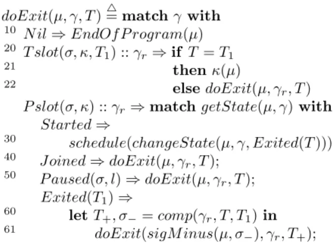
doExit(µ, γ, T )= match γ with4 10 N il ⇒ EndOf P rogram(µ) 20 T slot(σ, κ, T 1) :: γr⇒ if T = T1 21 then κ(µ) 22 else doExit(µ, γ r, T )
P slot(σ, κ) :: γr⇒ match getState(µ, γ) with
Started ⇒ 30 schedule(changeState(µ, γ, Exited(T ))) 40 J oined ⇒ doExit(µ, γ r, T ); 50 P aused(σ, l) ⇒ doExit(µ, γ r, T ); Exited(T1) ⇒ 60 let T +, σ−= comp(γr, T, T1) in 61 doExit(sigM inus(µ, σ −), γr, T+);
Figure 4: Synchronization with an exit
4.2
Synchronization
The three functions used in Figure 3, which do a pro-cess synchronisation, namely doExit, doP ause and doJ oin, receive as parameters a configuration and a stack. They perform a case analysis on the stack which can be empty or has on its top a slot left ei-ther by a tag or by a parallel. For a parallel slot, exactly two processes can make a synchronisation for this stack. The first incoming process will leave a trace on the stack, the last will make the final deci-sion. For reading and writing this trace we use the couple of functions getState and ChangeState. The initial state of a parallel slot is assumed to be Started (implicit in the slot creation P slot). Therefore, for these three functions, defined in figures 4, 5 and 6, finding a P slot on top of the stack with a Started state (line 30 for all functions) will change this state to a dedicated one and stop the process : the func-tion schedule takes a configurafunc-tion as argument and restarts one suspended process.
As expressed in Figure 4, an Exit on an empty stack is dynamically checked even if it is refused at compile time. An Exit(T ) without an encompassing T rap(T, . . .) is considered as aborting the whole com-putation according to the proofs of the next section. The objective of an Exit is to reach its correspond-ing T rap in the stack. There is one main case where unwinding the stack must be stopped : it occurs when
doP ause(µ, γ, σ, l)= match γ with4
10 N il ⇒ EndOf Instant(µ, σ, l) 20 T slot(σ, κ, T ) :: γ
r⇒ doP ause(µ, γr, σ, l)
P slot(σ, κ) :: γr⇒ match getState(µ, γ) with
Started ⇒
30 schedule(changeState(µ, γ, P aused(σ, l))) 40 J oined ⇒ doP ause(µ, γ
r, σ, l) 50 P aused(σ0, l0) ⇒ doP ause(µ
1, γr, σ + σ0, l • l0)
51 where µ
1= changeState(µ, γ, Started) 60 Exited(T ) ⇒ doExit(µ, γ
r, T );
Figure 5: Synchronization with a pause
a concurrent process wants also to exit (line 60 in fig 4), like in this pattern program :
trap T in trap T1 in (exit T kexit T1) end end
The process executing ”exit T ” and the one ex-ecuting ”exit T1” have the same stack, namely
P slot(σ1, κ1) :: T slot(σ2, κ2, T1) :: T slot(σ3, κ3, T ) ::
N il. The function comp returns the deepest tag name in the stack and the prediction associated to the low-est tag name. For the previous example, comp re-turns T and σ2. Since the exit of the lowest tag (T1)
is not effective, we have to decrement its associated prediction (σ2 or σ− in Figure 4, line 61)
The doP ause function (Figure 5) collects all the processes executing a pause. At a leaf of the tree of processes, when a process reaches a pause (fig 3, line 20), the function doP ause is called with the con-tinuation of the pause and the prediction for this process for the next instant. During the bottom-up traversal of the tree of processes (fig 5 line 50), the processes are appended in a list while the predictions are summed. One step of accumulation can be re-flected by the transformation :
pause;P1kpause;P2⇒ pause;(P1kP2)
At line 50, the two sets of processes l and l0 are still active (will continue to run in the next instant), therefore the P slot on top of the stack is still alive and thus must be reset with a Started trace (line 51) for the next instant. When the collection of con-tinuations ends at the root of the tree of processes (line 10), there is no more active process and we have reached the end of instant, i.e. all processes have
Using counters for absence prediction in Esterel 10
reached a pause. A new configuration can be made by incrementing the local time, setting the active pro-cesses with l and reseting the global prediction with σ. Note that when a process restarts, it retrieves automatically the stack it had when it was paused. This feature is due to the fact that stacks are closed under continuations. For example in fig 3 line 40, when evaluating the sequence P1;P2in a stack γ, the
evaluation of P2 will be evaluated in the same stack.
The T slots on the stack are only there to be caught by a corresponding Exit; therefore both doP ause and doJ oin (fig 6) will pop it by doing a recursion on the rest of the stack (line 20 on fig 5 and 6). This can be understood by the transformations :
trap T in pause;P end ⇒ pause;trap T in P end
and
trap T in N op end ⇒ N op.
One interesting situation is when one branch of a parallel is paused and the other is finished, as in the pattern :
pause;P knothing
One can consider that the parallelism must vanish and the previous statement reduced to ”pause;P ”. But the continuation of the paused process has closed the stack with the P slot on its top. It will be difficult and costly to remove this P slot in the interleaving of continuations. We will consider a lighter reduction of the previous statement with : ”pause;(P knothing)”. The P slot will stay on the stack but its state will never be changed in further instants and will remain as J oined. Note that this J oined state is forced when the paused process ar-rives first (fig 6 line 51) and otherwise is not changed (fig 5 line 40).
Recall (fig 2) that the prediction of the continu-ation of a parallel execution is injected in the two branches of the parallel statement. If these two branches terminate normally (i.e. doesn’t issue an exit) the prediction of the continuation is counted twice. Therefore, the first branch that completes its execution has to decrease the global prediction. This is done in the doJ oin function when a finished pro-cess arrives first at a Pslot (fig 6 line 30)
Finally, the ultimate goal of the synchronisation is reached in fig 6 line 40 when two processes have
doJ oin(µ, γ)= match γ with4
10 N il ⇒ EndOf P rogram(µ) 20 T slot(σ, κ, T ) :: γ
r⇒ doJ oin(µ, γr)
P slot(σ, κ) :: γr⇒ match getState(µ, γ) with 30 Started ⇒ schedule(sigM inus(µ
1, σ))
31 where µ
1= changeState(µ, γ, J oined) 40 J oined ⇒ κ(µ)
50 P aused(σ, l) ⇒ doP ause(σ
1, γr, σ, l)
51 where σ
1= sigM inus(µ1, σ)
51 where µ
1= changeState(µ, γ, J oined) 60 Exited(T ) ⇒ doExit(sigM inus(µ, σ), γ
r, T );
Figure 6: Synchronization with a join
completed the two branches of a parallel and when the continuation saved in the slot can be activated.
4.3
Waiting strategies
When a process reaches a ”present S” statement where the signal is not emitted and doesn’t have a count to 0, it has to wait (fig 3, line 63) via the stuck function. A first definition of this function could be simply :
stuck(S, µ, κ)= schedule(addW ork(µ, κ))4
It looks like a busy-waiting implementation. It seems better, and it is our current implementation, to have a specific set of waiting processes attached to signals. The stuck function simply adds the continua-tion to this set and proceeds with an other process via the schedule function. These waiting processes will be awaken as soon as the signal will be emitted, or when the counter of the signal becomes 0. This adds a test each time we emit a signal (fig 3 line 30) and an other test each time we decrement the count of a signal (inside of the sigM inus function). In return, however, the set of processes managed by the figuration, updated via the addW ork function, con-tains only active continuations. Therefore when the schedule function is called with a configuration con-taining an empty set of active process, we can infer a cyclic dependency between the waiting processes, and raise an error in this circumstance. For example, the following program, which only emit a signal in
the continuation of its presence test, will raise such an error :
present S then emit S else emit S end Some semantics of Esterel accept this program by considering the signal emitted a priori and by proving that considering the signal absent brings a contradic-tion. For this kind of program we assume that the user will rewrite the program by pulling up the emit before the test.
Coming back to the first definition of the stuck function, even if the waiting process is inserted again in the pool of processes, it may/must be the respon-sibility of the scheduler (i.e. the schedule function) to not pick up a new process arbitrarily. For example we can have two versions of the function addW ork. The first version, used at process creation (fig 3 line 52), will add the process on the left of the pool of processes, as if this pool had a LIFO-stack struc-ture. The second version, used in the stuck function, will add the process in the right of the pool as it had a FIFO-queue structure. The scheduler will use the pool as a stack when choosing a new candidate. This strategy doesn’t add extra tests in emit or in sigM inus, but a waiting process can still be asked to compute. Consider the following pattern of program :
present S1 then emit OK end
. . . kpresent Si+1 then emit Si end
. . . kemit Sn
of the form P1k . . . kPn+1. After the first round all the
processes but Pn+1are waiting for presence/absence
of a signal and the last process Pn+1has emitted the
signal Sn. At this point, the running list is P1. . . Pn
and only Pn can react to the emission of Sn.
There-fore this program will run in time proportional of n2 whereas using the commutativity of the
paral-lelism, the program Pn+1k . . . kP1will run in a linear
time. Moreover, with this implementation of waiting processes, it is not straightforward to decide when a cyclic dependency occurs.
4.4
Trampolines
Once written in CPS style, all significant calls of the evaluator are done in tail position. We can check in the figures 3 to 6 that the calls to eval, doExit, doP ause, doJ oin, schedule and all applications of
continuation are in tail positions. Even the func-tion EndOf Instant can be written with a tail call to schedule, with the appropriate new configuration as argument. Therefore, the execution of all programs can be done with a fixed bound of system stack.
It may appear that the implementation language, in which the evaluator is written, consume some stack space even for tail calls. In this case a trampoline technique must be used. It consists to return an ob-ject representing a function call instead of applying it. This object can be simply a thunk, a.k.a a function without argument. As an example, one can decide to clean the system stack each time a nothing is evalu-ated. Even if is not the better place to do it, we can change the line 10 in Figure 3 by λ .κ(µ), this frozen computation is directly returned to the first call of the evaluator. The main function calls the evalua-tor with the main statement and, while the answer is not the one given by EndOf P rogram, the frozen computation is restarted.
One can argue that adding a trampoline and find-ing places where to return thunks are implementation decisions and do not change the observation we can have on the computation : AST nodes are evaluated in the same order. But this equivalence helps to put in evidence some connections between different kinds of semantics. Without trampoline, the eval function defines a big step semantics of Esterel. If we return to the trampoline only inside the EndOf Instant func-tion, the eval function does the computation for one instant and is ready to be linked to standard opera-tional semantics. If we return to the trampoline ev-ery function call (except for functions like sigM inus, changeState,. . . ) we have switched to a small step semantics and the eval function, which is no more recursive, can be seen as defining a deterministic re-lation between configurations.
Since we have also specified this model of Esterel’s computation with the system Coq and knowing that it is not natural to define not well founded recursion, i.e. without a proof or termination, it was a chance to have this opportunity to switch to the equivalent small-step definition.
Using counters for absence prediction in Esterel 12
5
Coq specification
From the previous presentation, we have introduced several simplifications in order to prove the correct-ness of the specification in Coq. (1) we have aug-mented the semantics with some traces in order to express the correctness. (2) we have specialised the general type of continuations (function from configu-ration to answer) to a dedicated inductive type enu-merating the different kinds of continuations used by the semantics. This transformation is known as defunctionalization and described in [6] (3) we have unified the two passes prediction/evaluation by a single one where the evaluation recomputes, when needed, the prediction : a global prediction is no more used. (4) we have switched to a small step semantics where a step of computation is done by a (not re-cursive) function and the synchronisation is achieve by an inductive definition corresponding to a relation between configurations4. Finally we have proved the
correctness of the specification in this simplified def-inition.
5.1
Domains
The traces that executions may leave are of three kinds :
Inductive event : Set := | Emitted (s:name) | Present (s:name) | Absent (s:name).
At the end of an instant, a signal may be Emitted, considered as Present or considered as Absent. The correctness proof will insure that these three predi-cates are consistent, which mean essentially, that a message considered absent, with a counter valued to zero, must not be emitted . The evaluator will be tuned to generate events to a trace added to config-urations.
A configuration is a tuple containing the number of instants currently performed (getTime), the multi-set of processes (getWork) where a process is simply
4Since this relation doesn’t introduce difficulties in the
proofs, we will not describe it here.
a continuation (a multi-set is needed since two pro-cesses may have the same continuation as in P kP ), the function remembering the emitted signals for the current instant (getEmit), the current trace of events (getTrace). The last slot of configurations (getMax) is used to generate fresh variables.
Record config := Config { getTime : nat;
getWork : (list cont); getEmit : (name -> bool); getTrace : (list event) getMax : name;
}.
Then, for each explicit continuation expressed in Figure 3 (lines 40, 51, 52 and 71), for each direct recursive call to the evaluator in the same figure (lines 40, 53, 61, 62, 74, 80 and 100) and for each call to a synchronisation function (lines 20, 51 and 90) we create a dedicated inductive data structure.
Inductive cont : Set :=
| KStep (s:ast) (stk:(list slot)) (k:cont) | KLoop (s:ast) (stk:(list slot)) (t:nat) | KExit (stk:(list slot)) (t:name)
| KPause (stk:(list slot)) (l:(list cont)) | KJoin (stk:(list slot)).
The domain of slots is also an inductive type re-flecting the P slot and T slot expressed in the previous sections.
5.2
Specification
The main function of the specification is described in Figure 7 and is strongly related to the eval function given in Figure 3 receiving the same kind of param-eters. Let’s consider a configuration µ+ whose slot
getW ork is a list containing a continuation κ+of the
form KStep(P, γ, κ). Let’s consider the configuration µ identical to µ+ except for the slot getW ork where
the continuation κ+ is removed. In this state, the function step given in Figure 7 will be called with the arguments step(P, γ, µ, κ). Note that the con-figuration µ+ is rebuild line 61. The behaviour of step(P, γ, µ, κ) is to compute a new continuation κ1
step(P, γ, µ, κ)4= match P with 10 N op ⇒↓κ µ 20 P ause ⇒↓KP ause(γ,(κ::nil)) µ 30 Emit(S) ⇒↓κ addEvent(Emitted(S),changeSignal(µ,S,true)) 40 Seq(P 1, P2) ⇒↓ KStep(P1,γ,KStep(P2,γ,κ)) µ 50 P ar(P 1, P2) ⇒↓ KStep(P1,γ1,KJ oin(γ1))
addW ork(KStep(P2,γ1,KJ oin(γ1)),µ)
51 where γ
1= P slot(κ) :: γ 60 If (S, P
1, P2) ⇒
61 let µ+= addW ork(KStep(P, γ, κ), µ) in 62 match getEmit(µ, S), getKCount(µ+, S) with 63 true, ⇒↓KStep(P1,γ,κ)
addEvent(P resent(S),µ) 64 false, 0 ⇒↓KStep(P2,γ,κ)
addEvent(Absent(S),µ)
65 , ⇒ AStuck(µ)
70 Loop(P ) ⇒↓KStep(P,γ,KLoop(P,γ,getT ime(µ))) µ
80 T rap(T, P ) ⇒↓KStep(P,(T slot(κ,T )::γ),κ) µ 90 Exit(T ) ⇒↓KExit(γ,T ) µ 100 Signal(S, P ) ⇒↓KStep(rename(P,S,S1),γ,κ) µ1 101 where S 1, µ1= newSignal(µ)
Figure 7: simple evaluation
&S (κ) 4 = match κ with 10 KStep(P, γ, κ) ⇒S Π &S(κ) ⇓S(γ) P 20 KLoop(P, γ, time) ⇒S Π 0 ⇓S(γ)Loop(P ) 30 KExit(γ, T ) ⇒ cassq(T, ⇓ S (γ)) 40 KP ause(γ, l) ⇒ 0
50 KJ oin(γ) ⇒ getJ oinCounter(γ, S)
Figure 8: continuations to counters
corresponding to the rest of the computation after one step of evaluation of P in a stack γ and a contin-uation κ; step also generates a new configuration µ1
based on µ. Once κ1 and µ1 are build, the
continua-tion is added in the working list of µ1 and this final
configuration is returned; this is depicted by ↓κ1
µ1.
We have added insertion of events (lines 30, 63 and 64). Note lines 100 and 101, that we do not consider a complete renaming of signals. Thus, local signals are managed with fresh variables dynamically generated. The major difference, between the interpreter de-picted in fig 3 and the one implemented in Coq, is that a global prediction is no more considered and thus the functions sigM inus and sigAdd (lines 61, 62 and 73 of Figure 3) are no more used. Each process, and each continuation, is individually responsible of its prediction. If, for a given signal S, we consider a function &S (κ) from continuation to integer,
com-puting the counter for S for this continuation, then for a configuration the global counter is the sum of the continuation based counters for the continuations found in the working list :
getKCount(µ, S)4=P
κ∈getW ork(µ)&S(κ)
The correspondence between continuations and predictions is given in Figure 8. The crucial case if for a KStep(P, γ, κ) continuation, which need to be related to analyze(P, τ, σ) of Figure 2. Here γ is a list of slots (P slot or T slot) while τ is a mapping from tag names to predictions. It is easy to extract only T slot out of γ and, for each of them, to extract a counter via the continuation (using & ()) found in the T slot; this stack projection is done with the
Using counters for absence prediction in Esterel 14
function ⇓S (γ). The counter for a KJ oin(γ)
con-tinuation is computed with the concon-tinuation found in the first P slot in γ, or returns 0 if no P slot is found in γ.
Since for a continuation κ we need the counter for a specific signal S (&S (κ)), we have to specialise
the function analyze(P, τ, σ) for this signal. ΠS
a ρ P
computes the counter for S for the evaluation of P knowing that a is its counter for the continuation of P , ρ is a mapping from tag names to counters (imple-mented as list of associations for simplicity). There-fore, following Figure 2, we define ΠS
a
ρ P in Figure
9.
In this specification, we do not consider a com-plete renaming of the signals. It was simpler for the proofs not to characterise renamed programs. To avoid name conflicts, in Figure 7 line 100, each time a local signal definition is reached, a fresh signal name is generated. For the prediction (Figure 9 line 100), it is not trivial to going throw a local signal definition with the same name. In this case, the count of the continuation (i.e. a) seems correct but it would not consider the exceptions done by the body of the local definition. To be correct, this body must be analysed and the effect done on the local signal (i.e. ΠS
0 nil P )
must be discarded from the result. The key point is the nil parameter which avoid to consider the access to S outside of P via an exit.
5.3
Correctness
We have to prove that the events added by the evalu-ator are coherent, that is, a signal considered present will be emitted in the same instant, and conversely a signal considered as absent will not be emitted in the same instant. A configuration is well formed (W F (µ)) if it is reachable from an initial configu-ration build with a main statement.
Theorem 1 (correctness). : ∀µ, S, W F (µ) ⇒ [P resent(S) ∈ getT race(µ)
⇒ Emitted(S) ∈ getT race(µ)] ∧ [Absent(S) ∈ getT race(µ)
⇒ Emitted(S) 6∈ getT race(µ)]
S Π a ρP 4 = match P with 10 N op ⇒ a 20 P ause ⇒ 0 30 Emit(S 1) ⇒ if S1= S then a + 1 else a 40 Seq(P 1, P2) ⇒ s Π S Π a ρP2 ρ P1 50 P ar(P 1, P2) ⇒ s Π a ρP1+ S Π a ρ P2 60 If (A, P 1, P2) ⇒ s Π a ρP1+ S Π a ρ P2 70 Loop(P ) ⇒ΠS S Π 0 ρP ρ P 80 T rap(T, P ) ⇒S Π a (T ,a)::ρP 90 Exit(T ) ⇒ cassq(T, ρ) 100 Signal(S 1, P ) ⇒ S Π a ρP − ((S1= S) ? S Π 0 nilP : 0)
Figure 9: simple prediction of a signal
Proof. The first part is proved with the lemma getEmit(µ, S) = true ⇒ Emitted(S) ∈ getT race(µ) which is not difficult since the Emitted event is added in the same step where the status of the signal is changed (line 20 of Figure 7). The second part uses a proof by contradiction using the following lemma.
Lemma 1 (positive). A positive count is incompati-ble with an absent event :
∀µ, S, W F (µ) ⇒
getKCount(µ, S) > 0 ⇒ Absent(S) 6∈ getT race(µ). Proof. By induction on the step, induced by the W F definition, and by case analysis of the config-uration for a computational step. All cases, except loop, are not difficult since getKCount is generally decreasing with time. The end of an instant is trivial as the traces are reset. The major difficulty is for a loop which needs to prove that ΠS
0 ρ Loop(P ) ≥ S Π 0 ρ
Seq(P, Loop(P )) which is done by contradiction us-ing the followus-ing lemma.
Lemma 2 (null count conservation by loops). ∀P, ρ, S,
S Π S Π 0 ρP ρ P = 0 ⇒ S Π S Π S Π 0 ρ P ρ P ρ P = 0
Proof. This lemma cannot be proved directly by induction on P . We have to switch to a set of more general lemmas which have to be proved simultane-ously and which describe the variation ofΠs
a
ρ P on ρ
and a. Knowing thatΠs
a ρP = s Π 0 ρP + a ∗ k for some k,
we can apply this equality twice to prove our lemma.
Lemma 3 (Derivative of prediction). ∀P, ρ, a, s, Πs a ρP = s Π 0 ρP + a ∗ ∆F(P ) ∧ ∀P, ρ, a, s, Πs a (T ,c)::ρP = s Π a del(T ,ρ)P + c ∗ ∆E(P, T )
Proof. By induction on P . The function del removes all instances of the tag T in the list ρ. Note that an exit T without a surrounding ”trap T in end” is here considered as jumping to the end of the program. Even if this behaviour doesn’t appear at runtime, for the proof we consider that, at line 90 of Figure 9, the default value of cassq is 0. The function ∆F computes the number of control
paths that go through its argument in the same in-stant (i.e. without crossing a pause), while ∆E
com-putes the number of times that the evaluation of its first argument may exit with the tag given as second argument.
Here are the definitions of these two functions that are mutually recursive :
∆F(P ) 4 = match P with 10 N op ⇒ 1 20 P ause ⇒ 0 30 Emit(sig) ⇒ 1 40 Seq(P 1, P2) ⇒ ∆F(P1) ∗ ∆F(P2) 50 P ar(P 1, P2) ⇒ ∆F(P1) + ∆F(P2) 60 If (A, P 1, P2) ⇒ ∆F(P1) + ∆F(P2) 70 Loop(P ) ⇒ 0 80 T rap(T, P ) ⇒ ∆ F(P ) + ∆E(P, T ) 90 Exit(T ) ⇒ 0 100 Signal(sig, P ) ⇒ ∆ F(P ) ∆E(P, tag) 4 = match P with 10 N op ⇒ 0 20 P ause ⇒ 0 30 Emit(sig) ⇒ 0 40 Seq(P 1, P2) ⇒ ∆E(P1, T ) + ∆F(P1) ∗ ∆E(P2, T ) 50 P ar(P 1, P2) ⇒ ∆E(P1, tag) + ∆E(P2, tag) 60 If (A, P 1, P2) ⇒ ∆E(P1, tag) + ∆E(P2, tag) 70 Loop(P ) ⇒ (∆ F(P ) + 1) ∗ ∆E(P, tag) 80 T rap(T, P ) ⇒ (tag = T )?0 : ∆ E(P, tag) 90 Exit(T ) ⇒ (tag = T )?1 : 0 100 Signal(sig, P ) ⇒ ∆ E(P, tag)
6
Related work and
implemen-tations
In this section we consider the prediction analysis and the evaluator traditionnaly used in the synchronous language approach (subsection 6.1) and then we will give some details of the implementation (subsection 6.2).
6.1
Position
Positioning Esterel in the synchronous model is largely discussed in Attar’s thesis [1]. The closest area to Esterel is the reactive approach where the ab-sence of signals is not predicted but simultaneously established when no process can make a step of calcu-lus and the end of the instant is imposed. In this ap-proach there is always a delay of one instant between the evaluation of a test and of its else branch (when taken). The implementation of this reactive approach is really simpler since predictions are not needed. If we consider an implementation where waiting pro-cesses are attached to signals (see the discussion in 4.3), the case where the scheduler is called with an empty set of active processes is no more a cyclic de-pendency but simply the end of the instant. In this case, all the waiting processes come back in an active state knowing that the specific signal was absent in the previous instant. This approach is very attrac-tive, but there are still some programs that need to react without delay to absence. Think, for example, when one want to simulate a digital clocked circuit with each wire having its own signal. The presence of the signal acts as the hight level value in the wire,
Using counters for absence prediction in Esterel 16
the absence for the low level value. For example a negation for a wire in to a wire out is simply :
present in then nop else emit out end
Reacting instantaneously to the absence allows to maintain a direct relation between the clock of the circuit and the instants.
Using continuations for implementing/specifying synchronous languages is not widely adopted. The semantics is generally described by a structured op-erational semantics with term rewriting. The first use of continuations and of big step description seems to be attributed to L. Mandel [5] for the ReactiveML language. O. Tardieu and L. Mandel have also a, not (yet) published, interpreter, based on continuations, for a core of Esterel where the main ideas of our paper can be found. Instead of computing counters, list of lists of ”accessible” emitters are extracted from the source. The contribution of our paper is to do this extraction at compile time.
In [4], F. Boussinot extracts, through potential functions definitions, a hierarchy of semantics with refinement of absence detection. It seems that our interpreter falls in the ”v3” category.
6.2
Implementation
All the sources can be downloaded from ftp:ftp-sop.inria.fr/indes/rp/EsterelCounter.tar. The source code of the Coq specification is the file correct.v file. This file contains about 1500 lines with around 25% of definitions and 75% of proofs. The Scheme source code corresponding to the definitions found in Section 3 and Section 4 can be found in the file esterelSpec.scm and contains about 270 lines of code.
One remarkable characteristic of Esterel is the abil-ity to compile a program into a digital circuit. This implies that all objects can be allocated statically. This is the reason why predictions can be computed statically, but in fact everything can be preallocated before running the evaluation : the stack, the contin-uations, the signals, the waiting list associated to sig-nals, the running set of processes can actually be al-located statically. So we have implemented an inter-preter able to run using a fixed size of memory. The Scheme code of this implementation can be found in
the file esterelStatic.scm and contains about 830 line of code. Even if it is faster, this code is less readable than the previous version.
As stated in the beginning of the paper, Esterel is now candidate as an orchestration language with the implementation of HipHop [3] which is a layer of the Hop multi-tier language. We have also imple-mented a core of HipHop. The source code can be found in the file hiphop.scm which contains about 1600 lines of Scheme code. This code demonstrates that the extensions of HipHop can be handled with an implementation with counters, even with dynamic processes creation. The extensions proposed are :
1. Values. We have switched from statements to expressions, an expression returns a value. Any Scheme value can be introduced, as a constant, with the quote special form.
2. Valued signals. The emit special form accept an extra argument which is a value associated to the signal. The special form present is now the general Scheme test if. The presence/absence of a signal is tested with the special form now which return the true boolean (#t) when the sig-nal is present, false otherwise. All the values emitted by a signal can be founded with the spe-cial form val. The counters associated to signals are used to insure that all the values of a signal are already emitted. When a signal is not emit-ted and have a counter to 0, then it is known to be absent, but also when a signal is emitted and have a counter to 0 then we known that no more value can be emitted.
3. local variables. We have introduced local vari-ables declared with the let special form. The space need for these variables are preallocated and stored in the global memory.
4. Scheme access. All variables that cannot be re-solved as a local one are considered as a Scheme global variable. All Scheme value accessible through a global variable can be accessed in-side the reactive machine. This remains true for all global Scheme functions (+, string-ref, map. . . ). We have also introduced a node dedi-cated to call a Scheme function. An expression
like (+ 1 2) is valid in the reactive machine, also the more interesting expression (apply + (val sig)) which return the sum of all values emitted for the signal sig. The reactive ma-chine is not accessible to Scheme, thus the eval-uation of a Scheme code is instantaneous and cannot change the status of a signal. Evaluat-ing the arguments of a function can take several instants, for example, knowing that the pause special form return the logical time of the re-active machine, the expression (list (pause) ’quick (pause)) takes 3 instants and returns (1 quick 2)
5. Dynamic process creation. We have im-plemented the HipHop’s special form (mappar (lambda (x) P[x]) Vals) where, for each value x of the list computed by Vals, a pro-cess P, dependant of x, is created. All these processes P[x] run in parallel, may be within different instants, and join all together before the mappar returns all the computed values. The difficulty is to compute the counters for such expression. Consider for example the ex-pression (par (val s) (mappar (lambda (x) (emit s x)) (iota 5))). How the first pro-cess computing (val s) will know that all val-ues are emitted, as it depends on the length of the list computed by (iota 5)? Nevertheless, we can compute a common prediction σ for each process. In order to insure that at least one process is taken in account, the prediction σ is taken for the whole mappar expression, as if the computed list has a length of one. Dynamically, when the length n of the list is known, we read-just the global prediction with (n − 1) ∗ σ.
6. Dynamic process creation (cont). In the previous mappar special form, all the processes start in the same instant. We have implemented a more general special form (control Binds Body) where Binds is a list of bindings of the form (name (lambda (x) P[x])) where an ex-pression dependant of a variable x is associated to a name. Body may contains an expression of the form (detach (name Value)). Informally,
control acts as a pool of processes, initially con-taining only one process computing Body. Each time an expression (detach (name E)) is exe-cuted, a new process evaluating P[E] is added to the pool of processes. All the processes do a global synchronisation and all the computed val-ues are returned by the control special form. A prediction can be precomputed for each expres-sion in the Binds of the control. Then each time a detach is reached by the static analysis, the precomputed prediction is added.
7
Conclusion
We have presented a static analysis to let helps the interpreter of Esterel programs to decide the instan-taneous absence of a signal . The correctness of the analysis was formally proved. The analysis has been easily extended for a more functional language in-cluding dynamic process creation.
8
Acknowledgement
I would like to thank F. Boussinot for corrections and comments made on this report.
References
[1] Pejman Attar. Towards a Safe and Secure Syn-chronous Language. PhD thesis, Universit´e de Nice, 2013.
[2] G. Berry. The Constructive Semantics of Pure Esterel Draft Version 3. 2002.
[3] G´erard Berry, Cyprien Nicolas, and Manuel Ser-rano. Hiphop: a synchronous reactive extension for hop. In Proceedings of the 1st ACM SIG-PLAN international workshop on Programming language and systems technologies for internet clients, PLASTIC ’11, pages 49–56, New York, NY, USA, 2011. ACM.
Using counters for absence prediction in Esterel 18
[4] Fr´ed´eric Boussinot. SugarCubes Implementation of Causality. Technical Report RR-3487, INRIA, September 1998.
[5] Louis Mandel. Conception, S´emantique et Im-plantation de ReactiveML : un langage `a la ML pour la programmation r´eactive. PhD thesis, Uni-versit´e Paris 6, 2006.
[6] John C. Reynolds. Definitional interpreters for higher-order programming languages. In Reprinted from the proceedings of the 25th ACM National Conference, pages 717–740. ACM, 1972. [7] Olivier Tardieu and Robert de Simone. Curing schizophrenia by program rewriting in esterel. In MEMOCODE, pages 39–48. IEEE, 2004.
2004 route des Lucioles - BP 93 06902 Sophia Antipolis Cedex
BP 105 - 78153 Le Chesnay Cedex inria.fr