HAL Id: insu-02452723
https://hal-insu.archives-ouvertes.fr/insu-02452723
Submitted on 23 Jan 2020HAL is a multi-disciplinary open access archive for the deposit and dissemination of sci-entific research documents, whether they are pub-lished or not. The documents may come from teaching and research institutions in France or abroad, or from public or private research centers.
L’archive ouverte pluridisciplinaire HAL, est destinée au dépôt et à la diffusion de documents scientifiques de niveau recherche, publiés ou non, émanant des établissements d’enseignement et de recherche français ou étrangers, des laboratoires publics ou privés.
On viscoelastic regularisation of strain-softening rocks
and soils
René de Borst, Thibault Duretz
To cite this version:
René de Borst, Thibault Duretz. On viscoelastic regularisation of strain-softening rocks and soils. International Journal for Numerical and Analytical Methods in Geomechanics, Wiley, 2020, 44 (6), pp.890-903. �10.1002/nag.3046�. �insu-02452723�
DOI: xxx/xxxx
ARTICLE TYPE
On viscoplastic regularisation of strain-softening rocks and soils
René de Borst*
1| Thibault Duretz
21Department of Civil and Structural
Engineering, University of Sheffield, Sheffield, UK
2Univ Rennes, CNRS, Géosciences Rennes
UMR 6118, F-35000 Rennes, France
Correspondence
*René de Borst, Department of Civil and Structural Engineering, University of Sheffield, Sheffield S1 3JD, UK. Email: [email protected]
Funding information
Horizon 2020 European Research Council Grant 664734 "PoroFrac"
Summary
Constitutive models for rocks and soils typically incorporate some form of strain softening. Moreover, many plasticity models for frictional materials use a non-associated flow rule. Strain softening and non-non-associated flow rules can cause loss of well-posedness of the initial-value problem, which can lead to a severe mesh depen-dence in simulations and poor convergence of the iterative solution procedure. The inclusion of viscosity, which is a common property of materials, seems a natural way to restore well-posedness, but the mathematical properties of a rate-dependent model, and therefore the effectiveness with respect to the removal of mesh depen-dence, can depend strongly on how the viscous element is incorporated. Herein, we show that rate-dependent models which are commonly applied to problems in the Earth’s lithosphere, such as plate tectonics, is very different from the approach typically adopted for more shallow geotechnical engineering problems. We analyse the properties of these models under dynamic loadings, using dispersion analyses and one-dimensional finite difference analyses, and complement them with two-dimensional simulations of a typical strain localisation problem under quasi-static loading conditions. Finally, we point out that a combined model, which features two viscous elements, may be the best way forward for modelling time-dependent failure processes in the deeper layers of the Earth, since it enables modelling of the creep characteristics typical of long-term behaviour, but also regularises the initial/boundary-value problem.
KEYWORDS:
viscoplasticity, strain softening, regularisation, failure, non-associated flow
1
INTRODUCTION
Strain localisation occurs in all geological materials, for a wide range of length scales, varying from faults which are hundreds of kilometers long1,2, to decimeter-size laboratory samples3,4,5, and has been documented for a wide variety of materials, including
metals and marble, as early as 19316. Strain localisation refers to the phenomenon of the concentration of strains in narrow zones
when the applied load exceeds a certain threshold level. It not only manifests itself at a broad range of length scales, but also the temporal scales can differ widely. While for most buildings time-dependent deformations and the ensuing damage occur at the scale of several decades, geological processes within the lithosphere e.g., rock faults and shear zones, can stretch over millions of years.
Strain localisation poses a challenge to one of the cornerstones of classical continuum mechanics, namely the assumption that the mechanical and physical behaviour in a point is representative for a small, but finite volume surrounding it. This assumption,
while mostly correct, and ubiquitous in geomechanics and geophysics, fails for highly localised deformations, like fault move-ment or shear bands. A salient characteristic of the ensuing continuum is that it is devoid of an internal length scale, leading to the prediction of zero-width localisation bands.
In fact, much of the observed structural softening when testing, for instance, laboratory-sized specimens under smooth, well-controlled boundary conditions, is due to inhomogeneous deformations, in particular strain localisation, that develop in the specimen at failure4,5. The challenge is therefore to separate the observed structural softening into a contribution due to strain
localisation and another by the ’true’ material behaviour. The scale of this difficulty is illustrated by the simple example of non-associated plasticity. Even without the explicit introduction of strain softening at material level, i.e. for hardening or ideal plasticity, numerical simulations can show structural softening7,8,9,10,11.
In practice, the introduction of non-associated flow or strain softening at a material level is unavoidable when carrying out simulations based on the concept of a continuum. However, unless a continuum (plasticity) model which features strain soft-ening, or non-associated flow, is equipped with an internal length scale and can thus predict a finitely-sized localisation zone, it will lose ellipticity under (quasi)static loading conditions, and hyperbolicity under dynamic loading conditions, rendering the initial/boundary-value problem ill-posed. This observation is the underlying reason of the reported mesh sensitivity and the often erratic and unsatisfactory convergence behaviour of the equilibrium-searching iterative procedure12,13, which can be
aggravated upon mesh refinement14. A number of approaches have been proposed to repair this deficiency15, including Cosserat
plasticity16,17,18, non-local plasticity19,20,21and gradient plasticity22,23,24.
For a number of geomechanical applications, in particular those which involve very long-term processes in the Earth’s crust, the consideration of a deformation-limiting viscosity represents an alternative to non-local models. It is emphasised though, that not all rate-dependent rheologies solve the issue of mesh dependence, and that a pure series arrangement of the rheological elements25,26,27, which is typically used for modelling the Earth’s mantle or lithosphere, see Figure 1(a) for instance, does not
introduce a length scale and therefore does not remove the mesh dependence. By contrast, a plasticity model which relies on the introduction of a rate-limiting viscosity in a parallel arrangement with a plastic slider28,29, Figure 1(b), does introduce a length
scale and can therefore provide mesh-independent numerical solutions29,30.
The aim of this contribution is to elucidate that different elasto-visco-plastic rheologies lead to continuum descriptions which have very different mathematical properties. After a succinct recapitulation for a rate-independent elasto-plastic model, we derive the governing differential equation for each of the rate-dependent approaches in a one-dimensional context. We apply a dispersion analysis and verify this analysis with a finite difference computation. These analytical and numerical findings give insight in the possible dispersive properties of the wave propagation and the presence, or not, of an internal length scale, which is a condition for obtaining shear bands with a finite width. The analyses are augmented by two-dimensional finite difference analyses of shear band localisation under quasi-static loading conditions, and confirm the statements regarding mesh dependence for the two rate-dependent models. They also show an improved convergence behaviour of the (non-linear) iterative procedure for a well-posed problem. To point out a possible way forward in modelling time-dependent localised deformations in the deeper layers of the Earth’s crust, we have also examined a model which involves two viscous elements. Such a rheology can capture the viscous creeping mode as well as brittle yielding of deforming rocks.
2
DISPERSION ANALYSIS AND INTERNAL LENGTH SCALE
2.1
Rate-independent elasto-plasticity
We consider a one-dimensional bar with a uniform cross-section 𝐴 and a constant mass density 𝜌. Assuming small deformation gradients the balance of momentum is given by
𝜕𝜎 𝜕𝑥 = 𝜌
𝜕2𝑢
𝜕𝑡2 (1)
while the kinematic relation reads
𝜀= 𝜕𝑢
𝜕𝑥 (2)
with 𝜎 the axial stress and 𝑢 the axial displacement. As usual, 𝑥 and 𝑡 denote the spatial coordinate and time, respectively. As an introductory step, we consider a rate-independent elasto-plastic solid, so that after the onset of plastic yielding, i.e. when 𝜎 = 𝜎y, with 𝜎ythe yield strength, the strain 𝜀 can be partitioned into an elastic component and a plastic component, as follows:
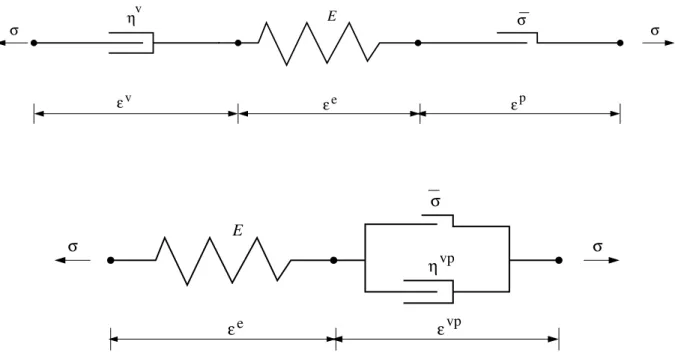
σ ε E e ε σ ε ηv v p σ ε E e σ η εvp vp σ σ
FIGURE 1 Rheological models: (a) Top: visco-elasto-plasticity; (b) Bottom: elasto-viscoplasticity
The stress is related to the elastic strain following Hooke’s relation, i.e.
𝜎= 𝐸𝜀e (4)
with 𝐸 the time and spatially independent Young’s modulus. In a one-dimensional context and for monotonic loading, the plastic strain rate can be derived by dividing the stress rate by the plastic hardening modulus ℎ:
̇𝜀p= ̇𝜎
ℎ (5)
Combining Eqs (3)–(5) leads to:
̇𝜎 = 𝐸ℎ
𝐸+ ℎ ̇𝜀 (6)
and combination with the momentum balance, Eq. (1) results in:
𝜌 (𝐸+ ℎ 𝐸 )𝜕2𝑢 𝜕𝑡2 = ℎ 𝜕2𝑢 𝜕𝑥2 (7)
Next, we assume a harmonic wave,
𝑢(𝑥, 𝑡) = 𝐴𝑒i(𝑘𝑥−𝜔𝑡) (8)
with 𝑘 the wave number counting the number of wave lengths𝓁 in the bar over 2𝜋, i.e. 𝑘 = 2𝜋∕𝓁, and 𝜔 the angular frequency.We substitute this expression into Eq. (7) to give:
𝜔= 𝑘 √
𝐸ℎ
𝜌(𝐸 + ℎ) (9)
or, using the definition for the phase velocity
𝑐𝑓 = 𝜔
𝑘 =
√
𝐸ℎ
𝜌(𝐸 + ℎ) (10)
A special case is the elastic bar velocity, which is obtained for a purely elastic material, i.e. ℎ → ∞, so that 𝑐𝑓 →
√
𝐸∕𝜌. The more important observation is that when ℎ < 0, the phase velocity becomes imaginary, implying non-real wave speeds and a wave propagation problem which is no longer hyperbolic, but elliptic, cf. Eq. (10)
2.2
Visco-elasto-plasticity
For sufficiently long time scales, all materials exhibit observable time-dependent deformations. For soft clays this holds for time scales that equal the life time of structures, while for hard rocks viscous behaviour shows up at geological time scales. For the
latter type of applications it has therefore become customary to include a viscous component in the description of rocks for their modelling at geological time scales25,26. The series arrangement of Eq. (3) is thus extended to include a viscous component:
̇𝜀v= 𝜎
𝜂v (11)
with 𝜂vthe viscosity of the material, such that:
𝜀= 𝜀e+ 𝜀p+ 𝜀v (12)
Using Eqs (4), (5), and (11) the strain rate reads:
̇𝜀= 𝐸+ ℎ
𝐸ℎ ̇𝜎+
𝜎
𝜂v (13)
Rearranging, differentiating with respect to 𝑥 and using the kinematic relation (2) gives:
𝜕2𝜎 𝜕𝑥𝜕𝑡 = 𝐸ℎ 𝐸+ ℎ ( 𝜕3𝑢 𝜕𝑥2𝜕𝑡 − 1 𝜂v 𝜕𝜎 𝜕𝑥 ) (14) Using the balance of momentum, Eq. (1) and integrating with respect to 𝑡 gives:
𝜕𝜎 𝜕𝑥 = 𝐸ℎ 𝐸+ ℎ ( 𝜕2𝑢 𝜕𝑥2 − 𝜌 𝜂v 𝜕𝑢 𝜕𝑡 ) (15) while using the balance of momentum again results in:
𝜌( 𝐸 𝐸+ ℎ )𝜕2𝑢 𝜕𝑡2 − ℎ 𝜕2𝑢 𝜕𝑥2 + 𝜌ℎ 𝜂v 𝜕𝑢 𝜕𝑡 = 0 (16)
Evidently, in the rate-independent limit, i.e. when 𝜂v→∞ the last term cancels and we retrieve the governing equation for an elasto-plastic solid, Eq. (7).
When comparing Eqs (7) and (16) it is clear that the viscous term in the rheological model has resulted in the addition of a first-order term in the governing equation. Since the character of a partial differential equation is determined by the higher-order terms31, no change is induced by this first-order term and it cannot be expected that the addition of the damper in the rheological
model will affect the change in character from hyperbolic to elliptic upon the introduction of strain softening (ℎ < 0). To further investigate this, we substitute a single, linear harmonic wave, Eq. (8), into Eq. (16). This results in:
−𝜌(𝐸 + ℎ)𝜔2+ 𝐸ℎ𝑘2−𝜌𝐸ℎ
𝜂v 𝜔i = 0 (17)
No solution is possible when the wave number 𝑘 is assumed to be real. Hence, we assume 𝑘 = 𝑘𝑟+ 𝛼i to be complex, which corresponds to the propagation of an exponentially attenuated harmonic wave:
𝑢(𝑥, 𝑡) = 𝐴𝑒−𝛼𝑥𝑒i(𝑘𝑟𝑥−𝜔𝑡) (18)
Substitution of the complex expression for 𝑘 into Eq. (17) and separating the resulting equation into real and imaginary parts gives:
−𝜌(𝐸 + ℎ) 𝜔2+ 𝐸ℎ(𝑘2𝑟 − 𝛼2) = 0 (19a)
𝑘𝑟𝛼−
𝜌𝜔
2𝜂v = 0 (19b)
Multiplying the first identity with 𝑘2𝑟and substituting the second identity allow to solve for 𝑘2𝑟:
𝑘2𝑟 = 𝜌𝜔 2(𝐸 + ℎ) 2𝐸ℎ ⎛ ⎜ ⎜ ⎝ 1 + √ 1 + 1 (𝜂v𝜔)2 ( 𝐸ℎ 𝐸+ ℎ )2⎞ ⎟ ⎟ ⎠ (20)
From the latter identity we directly obtain the phase velocity:
𝑐𝑓 = 𝜔 𝑘𝑟 = √ √ √ √ √ √ 2𝐸ℎ 𝜌(𝐸 + ℎ)⋅ 1 1 + √ 1 + 1 (𝜂v𝜔)2 (𝐸ℎ 𝐸+ℎ )2 (21)
In the absence of plastic straining, or when ℎ is positive, Eq. (21) shows that waves travel at a lower speed due to the presence of a damper because then 1
(𝜂v𝜔)2
(𝐸ℎ
𝐸+ℎ
)2
>0. Moreover, wave propagation is dispersive, since according to Eq. (21), the phase velocity 𝑐𝑓 is a function of 𝜔. Nevertheless, for strain softening, i.e. when ℎ < 0, the phase velocity still becomes imaginary.
The latter property is in line with the fact that there is no internal length scale in the visco-elastic-plastic model. Indeed, from the second identity of Eq. (19) we deduce that
𝛼= 𝜔 𝑘𝑟 ⋅ 𝜌 2𝜂v = 𝑐𝑓 𝜌 2𝜂v (22)
or, using Eq. (21)
𝛼= 𝜌 2𝜂v √ √ √ √ √ √ 2𝐸ℎ 𝜌(𝐸 + ℎ) ⋅ 1 1 + √ 1 + 1 (𝜂v𝜔)2 ( 𝐸ℎ 𝐸+ℎ )2 (23)
For the short-wave limit we thus have:
lim 𝜔→∞𝛼= √ 𝜌 2𝜂v √ 𝐸ℎ 𝐸+ ℎ (24)
which is imaginary for softening, thus precluding the presence of a real-valued internal length scale. The observation that this continuum model exhibits dispersive wave propagation, but does not have a real, non-zero internal length scale, and will therefore localise in a band of zero thickness at the onset of strain softening has been found before for a fluid-saturated porous medium32.
2.3
Elasto-viscoplasticity
An alternative rheological arrangement is to put a damper parallel to the plastic dissipative element, as shown in Figure 1(b). This type of arrangement is more common in engineering applications, and can for instance model the increase in strength at higher loading rates29. We depart from a decomposition of the strain into an elastic and a viscoplastic contribution, as follows:
𝜀= 𝜀e+ 𝜀vp (25)
The elastic strain is assumed to be related to the stress as in Eq. (4), and for the dashpot - plastic slider element we have:
𝜎= 𝜎𝑦+ ℎ𝜀vp+ 𝜂vṗ𝜀vp (26)
with 𝜎𝑦 the stress at the onset of plasticity, ℎ a constant hardening/softening modulus, and 𝜂vpis the viscosity of the dashpot.
Substitution of Eqs (2) and (4) into this identity, differentiating with respect to 𝑥 and using the momentum balance, Eq. (1), gives: 𝜌𝜕 2𝑢 𝜕𝑡2 = ℎ ( 𝜕2𝑢 𝜕𝑥2 − 1 𝐸 𝜕𝜎 𝜕𝑥 ) + 𝜂vp ( 𝜕3𝑢 𝜕𝑥2𝜕𝑡 − 1 𝐸 𝜕2𝜎 𝜕𝑥𝜕𝑡 ) (27) Using again the momentum balance and rearranging yields:
𝜂vp ( 𝜌 𝐸 𝜕3𝑢 𝜕𝑡3 − 𝜕3𝑢 𝜕𝑥2𝜕𝑡 ) + 𝜌𝐸+ ℎ 𝐸 𝜕2𝑢 𝜕𝑡2 − ℎ 𝜕2𝑢 𝜕𝑥2 = 0 (28)
This partial differential equation has third-order terms which determine its character. It has real characteristics, which enable the propagation of waves, and can therefore represent propagating waves, also when ℎ < 0.
The behaviour can be clarified further when carrying out a dispersion analysis as for the elasto-visco-plastic rheology29. We
again assume a harmonic wave which is attenuated exponentially when propagating through a one-dimensional bar, Eq. (18), substitute this expression into the governing partial differential equation (28), and separate real and imaginary parts. This leads to: 𝐸ℎ(𝑘2𝑟− 𝛼2) + 2𝜂vp𝜔𝐸𝑘𝑟𝛼− 𝜌(𝐸 + ℎ)𝜔2= 0 (29a) −𝜂vp𝜔𝐸(𝑘2𝑟 − 𝛼2) + 2𝐸ℎ𝑘𝑟𝛼+ 𝜌𝜂vp𝜔3 = 0 (29b) Summing up gives 𝑘𝑟𝛼= 𝜂 vp𝜔 2(ℎ2+ (𝜂vp)2𝜔2)𝜌𝜔 2 (30)
while substituting this identity into Eq. (29)𝑏, multiplying by 𝑘2𝑟, rearranging and finally solving for 𝑘2𝑟 yields:
𝑘2𝑟 = 𝜌𝜔 2 2𝐸 ⎛ ⎜ ⎜ ⎜ ⎝ (𝜂vp)2𝜔2+ ℎ2+ 𝐸ℎ +√((𝜂vp)2𝜔2+ ℎ2+ 𝐸ℎ)2+ (𝜂vp𝜔𝐸)2 (𝜂vp)2𝜔2+ ℎ2 ⎞ ⎟ ⎟ ⎟ ⎠ (31)
The phase velocity is thus obtained as: 𝑐𝑓 = 𝜔 𝑘𝑟 = √ √ √ √ √2𝐸𝜌 ⋅ (𝜂vp)2𝜔2+ ℎ2 (𝜂vp)2𝜔2+ ℎ2+ 𝐸ℎ +√((𝜂vp)2𝜔2+ ℎ2+ 𝐸ℎ)2+ (𝜂vp𝜔𝐸)2 (32)
which is clearly dispersive, and remains real for strain softening (ℎ < 0). Moreover, from Eq. (30) we obtain for the attenuation factor
𝛼= 𝑐𝑓 𝜌𝜂
vp𝜔2
2(ℎ2+ (𝜂vp)2𝜔2) (33)
One observes from Eq. (32) that
lim
𝜔→∞𝑐𝑓 = 𝑐𝑒=
√
𝐸
𝜌 (34)
the linear-elastic bar velocity, and since
lim 𝜔→∞ 𝜌𝜂vp𝜔2 2(ℎ2+ (𝜂vp)2𝜔2) = 𝜌 2𝜂vp (35) we obtain lim 𝜔→∞𝛼=𝓁 −1 (36)
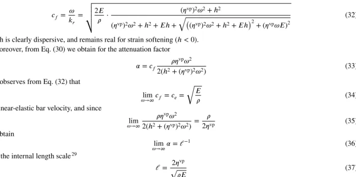
with the internal length scale29
𝓁 = 2𝜂
vp
√
𝜌𝐸
(37) Clearly, a visco-elasto-plastic model reacts very differently from an elasto-viscoplastic model, since unlike the latter, the former model is not equipped with an internal length scale. Importantly, the phase velocity in an visco-elasto-plastic continuum model becomes imaginary as soon as the hardening modulus turns negative, like in a standard elasto-plastic model, which is not the case for an elasto-viscoplastic model, where the wave speeds remain real.
σ ε E e ε σ η εvp vp σ ηv v
FIGURE 2 Visco-elasto-viscoplastic rheology
2.4
Visco-elastic-viscoplasticity
The deficiency of the elasto-viscoplastic model to properly describe long-term deformations at low to moderate stress levels by viscous creep can be repaired by added a damper in series to the spring and the viscoplastic element, Figure 2. The strain is now decomposed as:
𝜀= 𝜀v+ 𝜀e+ 𝜀vp (38)
where the stress in the viscoplastic element reads:
𝜎= 𝜎𝑦+ ℎ𝜀vp+ 𝜂vṗ𝜀vp (39)
while the stress in the spring and the other dashpot are given by Eqs (4) and (11), respectively. Differentiating with respect to the spatial coordinate and to time, using the momentum balance, Eq. (1), and the strain decomposition, Eq. (38), and substituting the constitutive equations, Eqs (4) and (11) yields:
𝜌𝜕 3𝑢 𝜕𝑡3 = ℎ ( 𝜕3𝑢 𝜕𝑥2𝜕𝑡− 1 𝐸 𝜕2𝜎 𝜕𝑥𝜕𝑡− 1 𝜂v 𝜕𝜎 𝜕𝑥 ) + 𝜂vp ( 𝜕4𝑢 𝜕𝑥2𝜕𝑡2 − 1 𝐸 𝜕3𝜎 𝜕𝑥𝜕𝑡2 − 1 𝜂v 𝜕2𝜎 𝜕𝑥𝜕𝑡 ) (40)
Again using the balance of momentum, integrating with respect to 𝑡 and rearranging yields the governing equation for the visco-elastic-viscoplastic model: 𝜂vp ( 𝜌 𝐸 𝜕3𝑢 𝜕𝑡3 − 𝜕3𝑢 𝜕𝑥2𝜕𝑡 ) + 𝜌 ( 𝐸+ ℎ 𝐸 + 𝜂vp 𝜂v ) 𝜕2𝑢 𝜕𝑡2 − ℎ 𝜕2𝑢 𝜕𝑥2 + 𝜌ℎ 𝜂v 𝜕𝑢 𝜕𝑡 = 0 (41)
When 𝜂v →∞, i.e. when the dashpot in series becomes fully rigid, the elasto-viscoplastic model is retrieved, Eq. (28). On the
other hand, when 𝜂vp →0, the visco-elasto-plastic model is obtained as a limiting case, Eq. (16). This again shows that having the dashpots in series or in parallel gives rise to a fundamentally different behaviour.
The analysis of dispersive waves in a visco-viscoplastic solid pretty much runs along the lines of that for an elastic-viscoplastic solid. We assume a single harmonic wave, which is damped exponentially upon propagation through the bar, Eq. (18), and substitute this expression into the governing partial differential equation, Eq. (41). Separating into real and imaginary parts now gives:
𝐸ℎ(𝑘2𝑟− 𝛼2) + 2𝜂vp𝜔𝐸𝑘𝑟𝛼− ( 𝜌(𝐸 + ℎ) +𝐸𝜌𝜂 vp 𝜂v ) 𝜔2= 0 (42a) −𝜂vp𝜔𝐸(𝑘2𝑟− 𝛼2) + 2𝐸ℎ𝑘𝑟𝛼+ 𝜌𝜂vp𝜔3− 𝜌𝐸ℎ 𝜂v 𝜔= 0 (42b)
Adding both expressions gives after reworking:
𝑘𝑟𝛼= 𝜂
vp𝜔
2(ℎ2+ (𝜂vp)2𝜔2)𝜌𝜔 2+ 𝜌𝜔
2𝜂v (43)
which reduces to Eqs (19)𝑏and (30) for 𝜂vp →0 and 𝜂v→∞, respectively. Substitution of this identity into Eq. (42)𝑏, multiplying
by 𝑘2
𝑟, and solving for 𝑘2𝑟 yields the dispersion relation, which can subsequently be used to derive the expression for the phase
velocity: 𝑐𝑓 = 𝜔 𝑘𝑟 = √ √ √ √ √ √ 2𝐸 𝜌 ⋅ (𝜂vp)2𝜔2+ ℎ2 (𝜂vp)2𝜔2+ ℎ2+ 𝐸ℎ + √ ( (𝜂vp)2𝜔2+ ℎ2+ 𝐸ℎ)2+ 𝐸2(𝜂vp𝜔+(𝜂vp)2𝜔2+ℎ2 𝜂v𝜔 )2 (44)
which remains real and positive when 𝜂vp ≠ 0 and reduces to the expressions for the wave velocities in the limiting cases of a visco-elasto-plastic solid, Eq. (21), and of an elasto-viscoplastic solid, Eq. (32), for 𝜂vp →0 and 𝜂v →∞, respectively. In the
short-wave limit, expression (44) turns into the elastic bar velocity: lim𝜔→∞𝑐𝑓 = 𝑐𝑒.
Similar to the elasto-viscoplastic solid, we can also here derive an internal length scale by considering the short wave-length limit. To this end, we rewrite Eq. (43) as:
𝛼= 𝑐𝑓 ( 𝜂vp𝜌𝜔2 2(ℎ2+ (𝜂vp)2𝜔2)+ 𝜌 2𝜂v ) (45) Defining lim𝜔→∞𝛼= 1
𝓁, with𝓁 the internal length scale, and considering that lim𝜔→∞𝑐𝑓 = 𝑐𝑒, the following expression can be
derived: 𝓁 = 2𝜂 vp𝜂v √ 𝜌𝐸(𝜂vp+ 𝜂v) (46) Clearly, for 𝜂v → ∞,𝓁 reduces to the expression obtained for an elasto-viscoplastic solid, Eq. (37), while for 𝜂vp → 0, a
vanishing length scale results, as expected.
3
ONE-DIMENSIONAL SIMULATIONS UNDER IMPACT LOADING
We now complement the theoretical findings of the preceding section with numerical simulations of a one-dimensional bar, which is subjected to an impact load at the left-hand side and fixed at the right-hand side. In this configuration a wave will start propagating from the left to the right in the bar and will double in intensity upon reflection.
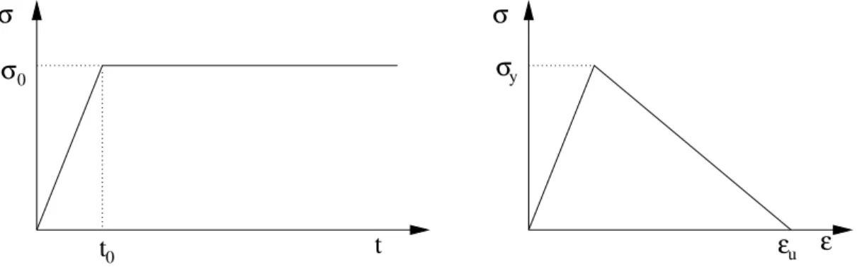
The load is applied during a rise time 𝑡0 = 0.05⋅ 10−3 s until a stress level 𝜎
0 = 19.9 Pa, which is marginally below the
compressive strength 𝜎y = 20 Pa, see also Figure 3. After reaching the compressive peak strength 𝜎, the strength linearly decreases to zero at an ultimate strain 𝜀u = 0.1. In all dynamic calculations the Young’s modulus is taken as 𝐸 = 20, 000 Pa and the mass density as 𝜌 = 1, 250 kg∕m3, resulting in an elastic bar velocity 𝑐
𝑒= 4 m∕s.
A fully explicit finite difference scheme has been used for the computations in order to avoid, or at least minimise numerical dispersion. The bar has a length 𝐿 = 1 m and is divided into 100 elements, unless mentioned otherwise. This leads to a critical
σ
σ
ε
ε
σ
t
0 uσ
yt
0FIGURE 3 Applied load as a function of time (left) and stress-strain diagram (right) for the simulations of wave propagation in a one-dimensional bar.
time step Δ𝑡crit= 0.01∕4 = 2.5⋅ 10−3s according to the Courant-Friedrichs-Lewy (CFL) criterion, which has been used in the
calculations for the elasto-viscoplastic model. Figure 5 confirms that in this case there is no dispersion during propagation of the elastic wave from the left-hand side until reflection at the right-hand side of the bar. For the calculation with a viscoelastic element, it appeared necessary to take a time step sligtly smaller, at Δ𝑡crit= 2.4975⋅ 10−3s to avoid numerical instabilities. This
is probably due to the introduction of viscosity during the propagation of the elastic wave. In fact, a marginally larger critical time step had been expected, since the viscoelastic wave propagates slower than the elastic wave, cf. Eq. (10) vs Eq. (21).
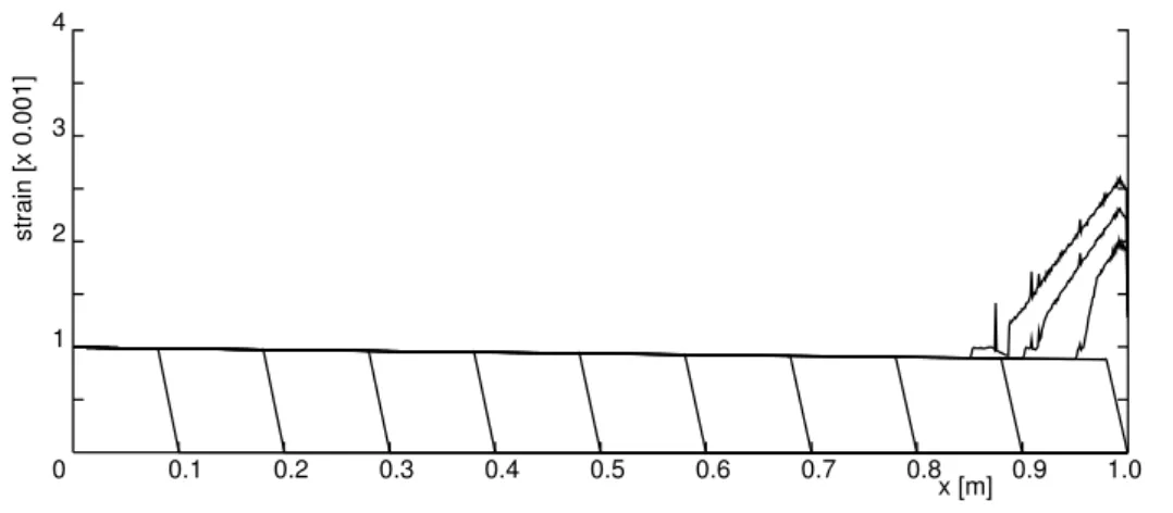
0 0.1 0.2 0.3 0.4 0.5 0.6 0.7 0.8 0.9 1.0 x [m] 1 2 3 4 strain [x 0.001]
FIGURE 4 Propagation and reflection of a wave modelled using the visco-elastic-plastic rheological model. The strain profile has been plotted after every 10 time steps.
The strain profiles which result from the computation for the visco-elasto-plastic model with a viscosity 𝜂v = 20, 000 Pa⋅ s have been plotted in Figure 4 at intervals of 10 time steps. It is observed that during propagation from the left-hand side of the bar to the right-hand side, the wave is attenuated, as predicted by Eq. (23). The lack of regularisation clearly shows up when the wave is reflected at the right-hand boundary, since the strain softening induced by the doubling of the stress intensity leads to deformation trapping in a single cell, with strains which theoretically become unbounded, but are controlled by the grid spacing in numerical simulations. For visibility purposes the Dirac-like strain has been chopped off at approximately half of the computed value in Figure 4.
Figure 5 shows that the response is fundamentally different for the elasto-viscoplastic model (𝜂vp = 103 Pa⋅ s). First, there
is no attenuation of the wave during propagation from the left to the right-hand side and numerical dispersion is absent since the critical time step could be chosen according to the CFL criterion. More importantly, upon reflection, the deformation is not
0 0.1 0.2 0.3 0.4 0.5 0.6 0.7 0.8 0.9 1.0 x [m] 1 2 3 4 strain [x 0.001]
FIGURE 5 Propagation and reflection of a wave modelled using the elasto-viscoplastic rheological model. The strain profile has been plotted after every 10 time steps before relection and for every 5 time steps afterwards.
trapped in a single cell as a wave starts to propagate to the left after reflection. Also, mesh refinement studies show a proper convergence behaviour29. The somewhat non-smooth strain profile of the travelling wave is mainly due to the relatively coarse
discretisation and disappears upon refinement of the discretisation.
0 0.1 0.2 0.3 0.4 0.5 0.6 0.7 0.8 0.9 1.0 x [m] 1 2 3 4 strain [x 0.001]
FIGURE 6 Propagation and reflection of a wave modelled using the visco-elastic-viscoplastic rheological model. The strain profile has been plotted after every 100 time steps before reflection and every 50 time steps after reflection.
The finite difference analysis has been repeated for the visco-elastic-viscoplastic model using the same material data. To mitigate the non-smooth strain profiles a finer discretisation has been used with 1000 cells and a concomitant time step Δ𝑡crit= 2.4975⋅ 10−4 s. The results are given in Figure 6 and, as expected, first show a wave which is attenuated when it propagates
from the left to the right, and, upon reflection, exhibit a propagating wave to the left with a real wave speed.
4
2D SIMULATIONS UNDER QUASI-STATIC LOADING CONDITIONS
To complement the one-dimensional simulations we now discuss a two-dimensional case which involves strain localisation13. Different from the previous studies the loading conditions are now quasi-static.
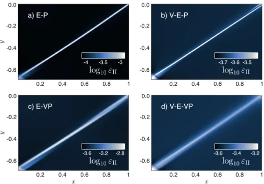
FIGURE 7 Spatial distribution of the second invariant of the accumulated strain after reaching a bulk strain of 3.0 × 10⁻⁴: (a)
Result obtained with an elasto-plastic model (E-P); (b) Result from a visco-elasto-plastic model (V-E-P); (c) Result obtained using an elasto-viscoplastic rheology (E-VP); (d) Results for a visco-elasto-viscoplastic rheology (V-E-VP)
.
We recognise that for quasi-static loading conditions a dispersion analysis cannot be carried out, and that therefore an internal length scale cannot, to the authors’ knowledge, be determined. In fact, the regularising effect of the viscosity, also when the damper is put in parallel to the plastic slider, will be weaker than under dynamic loadings, and will gradually disappear when the viscosity tends to zero. However, inclusion of a damper in parallel to the plastic dissipative element seems to lead to a diffusion-type equation, which is not the case for the elasto-plastic and visco-elasto-plastic models, and is probably the reason that for (visco)-elasto-viscoplastic models convergence to shear bands with a finite thickness is obtained. Nevertheless, numerical simulations seem to be the most rigorous way to assess whether convergence occurs upon mesh refinement, and therefore, whether the initial/boundary-value problem remains well-posed.
A rectangular domain of 1.0 m × 0.7 m is subjected to a kinematic boundary condition which induces a state of pure shear. The same number of nodes have been used in both spatial dimensions. Displacements increments Δ𝑢𝑥= −𝑥Δ𝜀, Δ𝑢𝑦= 𝑦Δ𝜀 are
imposed on the bottom and on the right-hand side of the domain, while the top and the left-hand boundaries are slip-free. The applied strain increment equals Δ𝜀 = 5.0 × 10⁻⁶. The initial stresses and strains have been set equal to zero. A circular inclusion with a radius 5 × 10⁻²m is located at the left-bottom corner. This imperfection is characterised by a 75% reduction of the shear
modulus.
An isotropic ideal-plasticity model has been used with a Drucker-Prager yield contour,
𝑓 =√𝐽2+ 𝑝 sin 𝜙 − 𝑐 cos 𝜙 (47)
and a non-associated flow rule such that the plastic potential function is given by:
𝑔=√𝐽2+ 𝑝 sin 𝜓 (48)
In Eqs (47) and (48) 𝑝 and 𝐽2are the first stress invariant and the second deviatoric stress invariant, respectively, while 𝜙 and 𝑐 measure the internal friction and the cohesion of the material, respectively. The factor 𝜓 sets the dilatancy of the material, i.e. the ratio between the plastic volumetric strain and the plastic deviatoric strain. The integration of the differential stress-strain rela-tion has been done using an implicit return mapping algorithm, while an algorithmic tangent operator obtained by consistently
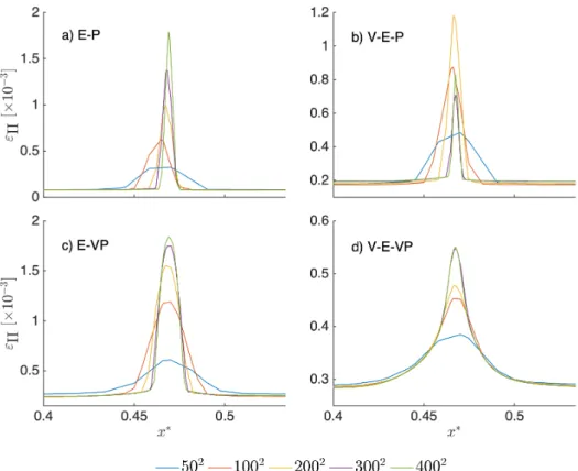
FIGURE 8 Strain profiles in terms of the second invariant of the accumulated strain (𝜀𝐼 𝐼) along a line normal to the shear band
for different discretisations: (a) Results for the elasto-plastic model; (b) Results for the elasto-visco-plastic model; (c) Results for the elasto-viscoplastic model; (d) Results for the elasto-viscoplastic model
.
linearising the integrated stress-strain relation has been utilised in a Newton-Raphson iterative procedure for obtaining equilib-rium. The numerical simulations have been carried out using the open source MATLAB code M2Di_EP33, which is based on
the M2Di routines34(https://bitbucket.org/lraess/m2di/src/master/).
In the calculations, the shear modulus 𝐺 has been set equal to 1 Pa and the bulk modulus 𝐾 = 2 Pa. A cohesion 𝑐 = 1.75×10⁻⁴Pa, an angle of internal friction 𝜙 = 30oand a dilancy angle 𝜓 = 10ohave been used as parameters for the plastic part. For the elasto-visco-plastic model the viscosity 𝜂v= 2.5×10⁵Pa⋅ s while for the elasto-viscoplastic model 𝜂vp= 2.5×10²Pa⋅ s.
The time step has been taken as Δ𝑡 = 104s, which yields a background strain rate ̇𝜀 =Δ𝜀
Δ𝑡 = 5.0 × 10 −9s−1.
It is noted that the non-associated flow rule utilised here causes a material instability and is the source of the loss of ellipticity and ensuing mesh dependence encountered in the calculations of the models with the elasto-plastic and visco-elasto-plastic rheologies10,14,35. In fact, it depends on the difference between the friction angle 𝜙 and the dilatancy angle 𝜓 , how severe the
consequences of this instability will be. Calculations have shown that when changing 𝜓 to 5o, respectively to 0othe regularising properties of the elasto-viscoplastic and visco-elasto-viscoplastic models were preserved13. On the other hand, for larger values
of 𝜓 shear banding could no longer be identified clearly.
For the elasto-plastic (E-P) and elasto-visco-plastic (E-V-P) models a shear localisation is computed with a width of approx-imately a single band of cells or elements. In these cases the numerical simulations fully depends on the discretisation. This phenomenon is commonly observed in calculations where loss of ellipticity occurs at a generic stage of the loading process. The strain localisation is visualised in Figures 7(a) and 7(b), where a mesh of 200 × 200 cells has been used. This is different for the elasto-viscoplastic and visco-elasto-viscoplastic models. Figures 7(c) and 7(d) show that shear localisation then spreads over several cells.
The differences between the different models can be brought out more clearly by presenting results for different levels of mesh refinement and plotting the strains along a line that is normal to the shear band. This has been done in Figure 8, which shows the second invariant of the strains along this line for all four models. Upon mesh refinement, the Dirac distribution-like character of the strain along this line is evident for the elasto-plastic and elasto-visco-plastic models. On the other hand,
convergence to a smooth, Gaussian-like strain distribution with a constant, finite width results from the computations with the elasto-viscoplastic and visco-elasto-viscoplastic models, although in the first case an even finer mesh would be necessary to attain full convergence. This indicates that the initial/boundary-value problem is now well-posed, and consequently, that results converge to a non-singular solution upon mesh refinement.
5
CONCLUDING REMARKS
We have discussed the consequences of placing a dashpot either in series or in parallel to a plastic dissipative element. It turns out that when the plastic slider is equipped with strain softening behaviour, a parallel arrangement is essential, since the alternative of a series arrangement will lead to a vanishing internal length scale with the concomitant consequences of localisation into a zero band width upon failure and imaginary wave speeds under dynamic loading conditions in the plastified, softening zone. This has been proven analytically using dispersion analyses of wave propagation and has been further corroborated with simulations of dynamic loadings, which show a strain singularity in the form of a Dirac function upon failure, indicating a local loss of hyperbolicity of the governing equations. This implies that well-posedness of the initial-value problem ceases to hold.
A crucial requirement for localisation to occur in a band of finite width is the existence of a non-vanishing internal length scale in the continuum. We have rigorously shown that this is the case for the elasto-viscoplastic and visco-elastic-viscoplastic models under dynamic loading conditions, and have derived explicit expressions for 1D boundary value problems. While the 2D numerical simulations in this paper and elsewhere13indicate that a non-vanishing length scale also exist under quasi-static loading conditions, under proviso of course that the viscosity of the element parallel to the slider is non-zero, a formal proof does not seem to exist. In particular, it is unlikely that the derived expressions for the internal length scale extend to multidimensional boundary value problems under quasi-static loading conditions.
The above observations have consequences for the modelling of soils, and particularly rocks at geological time scales. Models in which a plastic slider is put in series with a dashpot are commonly used in computational models of the lithosphere, as they are necessary to capture essential features at short timescales36,37,38as well as strain localisation at long timescales25,39,40,41. At the same time, such models can be mathematically deficient, as we have shown, and may not yield reliable numerical predic-tions for faulting, folding, or necking phenomena in the plastic realm. In combination with strain softening or a non-associated flow, numerical solutions are inherently mesh sensitive and often fails to reach mechanical equilibrium12. These drawbacks are
independent of the employed discretisation and occur either using finite difference, finite element, or meshless methods.14,42. A promising way forward is to combine visco-elasto-plastic and elasto-viscoplastic rheological models. We have shown that a rheology which has a dashpot in series to the plastic slider as well as a dashpot in parallel to the plastic slider enjoys the benefits of both modelling approaches. It is equipped with an internal length scale, which prevents localisation into a band of zero width, and possesses real wave speeds also in the softening regime. At the same time it is in principle capable of properly capturing the time-dependent behaviour of rocks, both for shorter timescales and for longer timescales.
An open issue is how to determine the viscosities of the dashpots. Probably, the dashpot in series can be calibrated in the usual way from creep experiments43. For the dashpot which is in parallel to the plastic slider may be extracted from deformation
experiments44, or used as a user-defined regularisation parameter for strain localisation. In the latter case a calibration using numerical experiments may be necessary.
Finally, we recognise that the linear dashpots used in the present study are oversimplified and that more advanced theories such as power-law creep, exponential creep and temperature or strain-dependent creep would better capture the long-term rhe-ological behaviour of rocks45. However, this does not affect our conclusion that in order to have predictive simulations which are independent of the discretisation, rheologies which have a dashpot-like element in series with a plastic dissipative element, must be augmented with a dashpot-like element with is put in parallel to the plastic slider.
Acknowledgement
References
1. McKenzie DP. Plate tectonics of the Mediterranean region. Nature 1970; 226: 239–243. 2. Anderson DL. The San Andreas fault. Scientific American 1971; 225: 52–71.
3. Paterson MS. Experimental deformation and faulting in Wombeyan mable. GSA Bulletin 1958; 69: 465-476.
4. Desrues J, Chambon R, Mokni M, Mazerolle F. Void ratio evolution inside shear bands in triaxial sand specimens studied by computed tomography. Géotechnique 1996; 46: 529–546.
5. Desrues J, Viggiani G. Strain localization in sand: an overview of the experimental results obtained in Grenoble using stereophotogrammetry. International Journal for Numerical and Analytical Methods in Geomechanics 2004; 28: 279–321. 6. Nadai A. Plasticity. New York and London: McGraw-Hill . 1931.
7. Vermeer PA, de Borst R. Non-associated plasticity for soils, concrete and rock. Heron 1984; 29(3): 3–64.
8. de Borst R. Bifurcations in finite element models with a non-associated flow law. International Journal for Numerical and
Analytical Methods in Geomechanics1988; 12: 99–116.
9. Le Pourhiet L. Strain localization due to structural softening during pressure sensitive rate independent yielding. Bulletin
de la Société géologique de France2013; 184: 357-371.
10. Sabet SA, de Borst R. Structural softening, mesh dependence, and regularisation in non-associated plastic flow. International
Journal for Numerical and Analytical Methods in Geomechanics2019; 43: 2170–2183.
11. Yamato P, Duretz T, Angiboust S. Brittle/ductile deformation of eclogites: Insights from numerical models. Geochemistry,
Geophysics, Geosystems2019; 20: 3116–3133.
12. Spiegelman M, May DA, Wilson CR. On the solvability of incompressible Stokes with viscoplastic rheologies in geodynamics. Geochemistry, Geophysics, Geosystems 2016; 17: 2213–2238.
13. Duretz T, de Borst R, Le Pourhiet L. On finite thickness of shear bands in frictional viscoplasticity, and implications for lithosphere dynamics. Geochemistry, Geophysics, Geosystems 2019(2019GC008531).
14. de Borst R, Crisfield MA, Remmers JJC, Verhoosel CV. Non-Linear Finite Element Analysis of Solids and Structures. Chichester: Wiley. second ed. 2012.
15. de Borst R, Sluys LJ, Mühlhaus HB, Pamin J. Fundamental issues in finite element analysis of localisation of deformation.
Engineering Computations1993; 10: 99–122.
16. Mühlhaus HB, Vardoulakis I. The thickness of shear bands in granular materials. Géotechnique 1987; 37: 271-283. 17. de Borst R, Sluys LJ. Localisation in a Cosserat continuum under static and dynamic loading conditions. Computer Methods
in Applied Mechanics and Engineering1991; 90: 805–827.
18. Stefanou I, Sulem J, Rattez H. Cosserat approach to localization in geomaterials. In: Voyiadjis GZ. , ed. Handbook of
Nonlocal Continuum Mechanics for Materials and StructuresBerlin: Springer. 2019 (pp. 1–25).
19. Bažant ZP, Lin FB. Non-local yield limit degradation. International Journal for Numerical Methods in Engineering 1988; 26: 1805–1823.
20. Strömberg L, Ristinmaa M. FE-formulation of a nonlocal plasticity theory. Computer Methods in Applied Mechanics and
Engineering1996; 136: 127–144.
21. Bažant ZP, Jirasek M. Nonlocal integral formulations of plasticity and damage: Survey of progress. Journal of Engineering
22. de Borst R, Mühlhaus HB. Gradient-dependent plasticity: Formulation and algorithmic aspects. International Journal for
Numerical Methods in Engineering1992; 35: 521-539.
23. Kolo I, de Borst R. An isogeometric analysis approach to gradient-dependent plasticity. International Journal for Numerical
Methods in Engineering2018; 113: 296–310.
24. Kolo I, de Borst R. Dispersion and isogeometric analyses of second-order and fourth-order implicit gradient-enhanced plasticity models. International Journal for Numerical Methods in Engineering 2018; 114: 431–453.
25. Gerya TV, Yuen DA. Robust characteristics method for modelling multiphase visco-elasto-plastic thermo-mechanical problems. Physics of the Earth and Planetary Interiors 2007; 163: 83–105.
26. Lemiale V, Mühlhaus HB, Moresi L, Stafford J. Shear banding analysis of plastic models formulated for incompressible viscous flows. Physics of the Earth and Planetary Interiors 2008; 171: 177-186.
27. Kaus BJP. Factors that control the angle of shear bands in geodynamic numerical models of brittle deformation.
Tectonophysics2010; 484: 36–47.
28. Perzyna P. Fundamental problems in viscoplasticity. In: Cherny GG., ed. Recent Advances in Applied Mechanics. 9. New York: Academic Press. 1966 (pp. 243–377).
29. Sluys LJ, de Borst R. Wave propagation and localization in a rate-dependent cracked medium – model formulation and one-dimensional examples. International Journal of Solids and Structures 1992; 29: 2945–2958.
30. Wang WM, Sluys LJ, de Borst R. Interaction between material length scale and imperfection size for localisation phenomena in viscoplastic media. European Journal of Mechanics. A, Solids 1996; 15: 447–464.
31. Courant R, Hilbert D. Methoden der Mathematischen Physik. II. Berlin: Verlag Julius Springer . 1937.
32. Abellan MA, de Borst R. Wave propagation and localisation in a softening two-phase medium. Computer Methods in Applied
Mechanics and Engineering2006; 195: 5011–5019.
33. Duretz T, Souche A, de Borst R, Le Pourhiet L. The benefits of using a consistent tangent operator for viscoelastoplastic computations in geodynamics. Geochemistry, Geophysics, Geosystems 2018; 19: 4904–4924.
34. Räss L, Duretz T, Podladchikov YY, Schmalholz SM. M2Di: Concise and efficient MATLAB 2-D Stokes solvers using the Finite Difference Method. Geochemistry, Geophysics, Geosystems 2017; 18: 755-768.
35. Rudnicki JW, Rice JR. Conditions for the localization of deformation in pressure sensitive dilatant materials. Journal of the
Mechanics and Physics of Solids1975; 23: 371–394.
36. Deng J, Gurnis M, Kanamori H, Hauksson E. Viscoelastic flow in the lower crust after the 1992 Landers, California, Earthquake. Science 1998; 282: 1689–1692.
37. Heimpel M. Earthquake scaling: the effect of a viscoelastic asthenosphere. Geophysical Journal International 2006; 166: 170-178.
38. Wang K. Elastic and viscoelastic models of crustal deformation in subduction earthquake cycles. In: Dixon T, Moore JC., eds. The Seismogenic Zone of Subduction Thrust FaultsNew York: Columbia University Press. 2007 (pp. 540–575). 39. Moresi L, Dufour F, Mühlhaus HB. Mantle convection modeling with viscoelastic/brittle lithosphere: Numerical
method-ology and plate tectonic modeling. Pure and Applied Geophysics 2002; 159: 2335–2356.
40. Popov AA, Sobolev SV. SLIM3D: A tool for three-dimensional thermomechanical modeling of lithospheric deformation with elasto-visco-plastic rheology. Physics of the Earth and Planetary Interiors 2008; 171: 55–75.
41. Buiter SJH, Schreurs G, Albertz M, et al. Benchmarking numerical models of brittle thrust wedges. Journal of Structural
42. Askes H, Pamin J, de Borst R. Dispersion analysis and element-free Galerkin solutions of second and fourth-order gradient-enhanced damage models. International Journal for Numerical Methods in Engineering 2000; 49: 811–823.
43. Weertman J, Weertman JR. High temperature creep of rock and mantle viscosity. Annual Review of Earth and Planetary
Sciences1975; 3: 293-315.
44. Cristescu N. Elastic/viscoplastic constitutive equations for rock. International Journal of Rock Mechanics and Mining
Sciences & Geomechanical Abstracts1987; 24: 271 –282.
45. Karato S. Deformation of Earth Materials: An Introduction to the Rheology of Solid Earth. Cambridge: Cambridge University Press . 2008.