HAL Id: hal-03080901
https://hal.archives-ouvertes.fr/hal-03080901
Submitted on 17 Dec 2020HAL is a multi-disciplinary open access
archive for the deposit and dissemination of sci-entific research documents, whether they are pub-lished or not. The documents may come from teaching and research institutions in France or abroad, or from public or private research centers.
L’archive ouverte pluridisciplinaire HAL, est destinée au dépôt et à la diffusion de documents scientifiques de niveau recherche, publiés ou non, émanant des établissements d’enseignement et de recherche français ou étrangers, des laboratoires publics ou privés.
observations and surface processes
Severine Rosat, N Gillet, Jean-Paul Boy, A Couhert, M Dumberry
To cite this version:
Severine Rosat, N Gillet, Jean-Paul Boy, A Couhert, M Dumberry. Interannual variations of de-gree 2 from geodetic observations and surface processes. Geophysical Journal International, Oxford University Press (OUP), 2020, �10.1093/gji/ggaa590�. �hal-03080901�
Interannual variations of degree 2 from geodetic
observations and surface processes
S. Rosat
1,∗, N. Gillet
2, J.-P. Boy
1, A. Couhert
3, M. Dumberry
41Universit´e de Strasbourg, CNRS, EOST, IPGS UMR 7516, F-67000 Strasbourg, France
2Univ. Grenoble Alpes, Univ. Savoie Mont Blanc, CNRS, IRD, IFSTTAR, ISTerre, F-38000 Grenoble, France 3Centre National d’Etudes Spatiales, 18 avenue Edouard Belin, 31401 Toulouse, France
4Department of Physics, University of Alberta, Edmonton T6G 2E1, Canada
*Email: [email protected]
SUMMARY
Geodetic observations from space continuously record surface deformation and global mass redistribution with an increasing accuracy. In parallel, surficial processes (oceanic, atmospheric, and hydrological loading) are more and more precisely modeled. We pro-pose a confrontation of the geodetic Global Positioning System (GPS) and gravity-field satellite laser ranging (SLR) observations at decadal and interannual time scales, in terms of resolution, correlation and comparison with surficial loading models. We focus on the largest global scale signals of degree 2. At interannual periods, surface deforma-tions retrieved from GPS time-series do not exceed 0.8 mm. Our analysis does not reveal the presence of a dominant signal at a specific period, except perhaps for a signal of approximately 3 yr likely connected to the loading response to El Ni˜no / Southern Os-cillations. Contrary to the results of previous studies, we do not find in GPS time-series a clear 6-yr oscillation associated with a degree-2 order-2 pattern. Interannual variations in the degree-2 Stokes coefficients of the gravity field do not exceed 2 × 10⁻¹¹. We do not detect a dominant gravity signal at one specific period but instead a broad spectrum of frequencies. The comparison between the degree 2 deformations built from GPS
time-series with a prediction from SLR derived gravity variations reveals some correlations, though their differences remain important. This highlights the present day limitations of these techniques in their ability to characterize global scale interannual variations. Hydrological loading models show some correlations with both GPS and SLR signals, but we cannot firmly establish that continental hydrology is dominantly responsible for the observed variations. Given the current limits in the resolution of both gravity and surface deformation and in the modelling of surface processes, we conclude that it will be a challenge to retrieve a geodetic signal of sub-decadal period originating in the Earth’s core.
Key words: Satellite geodesy – Satellite gravity – Loading of the Earth – Global change from geodesy – core – Time-series analysis
1 INTRODUCTION
Surface deformations are continuously recorded from space by Global Navigation Satellite System (GNSS) fleet of satellites with steadily improving accuracy. Vertical and horizontal displacements recorded at ground stations are from a variety of sources and occur over a vast range of spatial and temporal scales. This includes for instance the post-glacial rebound, tidal deformations, surficial loading from fluid layers, co- and postseismic as well as volcanic deformations. The temporal scales involved range from seconds to years, and the spatial scales from millimeters to continental dimension. Variations in the Earth’s gravity field are also monitored with an increasing accuracy by space geodetic measurements. This includes the Gravity Recovery and Climate Experiment (GRACE), satellite laser ranging (SLR), and Earth rotation (see e.g. Chen et al. 2016).
At seasonal and shorter time-scales, the largest global deformations are produced by tidal forces and loading from surficial layers (atmosphere, oceans and continental hydrology). The connection between hydrological processes and gravity field measurements has been widely investigated since the launch of GRACE satellite mission between August 2002 and June 2017 and by the GRACE Follow-On satellite mission starting June 2018 (see e.g. Tapley
et al. 2004, 2019). The contribution of seasonal (annual and semi-annual) surface mass redistribution has also proved to be a dominant part of the signal in the observed Global Positioning System (GPS) vertical displacements (e.g. van Dam et al. 2001; Dong et al. 2002; Memin et al. 2020). Seasonal mass redistributions were also studied by joint analyses of GPS and GRACE or SLR observations showing consistent results (Collilieux et al. 2007; Fu et al. 2012; Zou et al. 2015) and in agreement with loading models (Nahmani et al. 2012; Chanard et al. 2018), although systematic differences appear to be present (Kusche & Schrama 2005). Although the focus has been on annual and sub-annual timescales, GPS observations go back for two decades (Bock & Melgar 2016; Larson 2019), and satellite measurement of gravity for three decades (Bloßfeld et al. 2018). Longer timescale changes can be investigated. Changes in Earth’s dynamic oblateness have been inspected (e.g. Cox & Chao 2002; Nerem & Wahr 2011; Cheng et al. 2013; Loomis et al. 2019), but also variations in the Earth’s figure axis in their connection to polar motion (e.g. Chen & Wilson 2005; Cheng et al. 2011; Adhikari & Ivins 2016). These studies are more focused on trends: they showed that changes in degree-2 gravity field are dominantly driven by surface processes.
Interannual variations have received less attention, although a few recent studies have identified specific GPS and gravity signals of harmonic degree 2 at a period close to 6 yr. First, both Ding & Chao (2018) and Watkins et al. (2018) have highlighted the presence of a 5.9-yr signal in GPS observations. More specifically, the signal identified in Ding & Chao (2018) corresponds to a 1.7 mm amplitude degree-2 order-2 pattern in vertical displacement, travelling westward and completing a half-rotation (and a full periodic cycle at a given point on the surface) in 5.9 years. A connected westward travelling signal in the degree-2 order-2 pattern of the gravity field was isolated from SLR gravity measurements (Chao & Yu 2020). Furthermore, Chen et al. (2019) detected interannual oscillations in polar motion which are connected to the degree-2 order-1 components of the gravity field.
In each of these studies, the origin of the identified signals was suggested to be from dynamical processes in the Earth’s core. The rationale for this stems from an observed 5.9 yr variation of the length-of-day (LOD) (Abarca del Rio et al. 2000; Chen et al. 2005;
Holme & De Viron 2013; Chao et al. 2014) which has been shown to be caused by an angular momentum exchange between the core and the mantle (Gillet et al. 2010, 2019). Processes in the Earth’s core, the logic goes, are then possibly responsible for the observed changes in vertical displacement, gravity and polar motion at the same period.
Gravity changes and vertical displacements at the Earth’s surface can result from differ-ent core processes. First, core flows generate lateral pressure variations at the core-mantle boundary (CMB). To maintain mechanical equilibrium, these CMB pressure changes induce global elastic deformations, including at the surface, and the mass displacements associated with these lead to an alteration of the gravity field (Fang et al. 1996; Greff-Lefftz et al. 2004; Dumberry & Bloxham 2004). Second, density heterogeneities involved in convective core motions also lead to changes in the global gravity field and to elastic deformations (Dumberry 2010). Third, an axial or equatorial rotation of the solid inner core, because of its ellipsoidal shape and the density contrast at the inner core boundary, produces changes in the degree-2 gravity field (Dumberry & Bloxham 2004; Chao 2017).
Flows near the top of the core can be partly reconstructed by inversion from the observed temporal changes of the Earth’s magnetic field. Decadal and subdecadal changes in LOD offer an additional constraint on the reconstructed flows. If indeed GPS and gravity observations contain signals of core origin, these would provide further constraints on flows and dynamical processes within the Earth’s core. However, before such a conclusion can be reached, it is important first to validate that the geodetic signals are sufficiently robust. In addition, it is also important to ensure that surface processes are not responsible for these signals. It is only once all surface processes are correctly accounted for that an inference on the deep Earth’s dynamics can be carried out.
The objectives of this paper are to present an up-to-date description of the degree-2 changes in GPS and gravity field observations from SLR, and a comparison with geophysical models of surface loading, focusing on interannual periods. We want to asses to what degree the current models of surface processes are capable to explain the planetary scale interannual
variations recorded in GPS and SLR observations. In light of the earlier studies mentioned above, we place a particular emphasis on signals with a period close to 6 yr.
We first present the results of the analysis of nearly 20 years of GPS displacement time-series. A confrontation with non-tidal atmospheric, oceanic and hydrological loading products is presented. Three decades of gravity variations, in the form of variations in the Stokes coefficients from SLR, complete the analysis. We then focus on the degree-2 vertical displacements around 6 yr from GPS and SLR observations and from hydrological loading. Finally, we discuss the consistency between the different approaches, and the possibility of retrieving in geodetic observations signals associated with deep Earth’s processes at decadal and interannual time scales.
2 GEODETIC OBSERVATIONS AND PRE-PROCESSING
2.1 GNSS vertical displacements
We have considered two datasets of GPS time-series, one from the JPL (Jet Propulsion Laboratory, California Institute of Technology) and one from the international GNSS service (IGS).
The JPL solution is produced using the GipsyX software in a Precise Point Positioning mode (Heflin et al. 2020). All individual solutions are aligned with the IGS14 terrestrial reference frame. Time-series were corrected for the seasonal (annual and semi-annual) terms and the solid and ocean tidal signals. We consider the residual time-series which have been corrected for offsets and outliers as described in Heflin et al. (2020). From the selection of the longest timeseries with common time-windows, we finally keep 83 time-records of duration 19.8 years (Feb. 1999 - Dec. 2018) with a geographical distribution shown in Fig. 1a.
The IGS solution is based on the reprocessing of daily GNSS (GPS and eventually GLONASS) solutions (including station position, LOD and Polar Motion) from 8 different analysis centers for the Repro2 campaign. Position time-series were analyzed station by sta-tion to identify discontinuities, velocity changes and post-seismic deformasta-tions (modelled by exponential and/or logarithmic functions). These daily solutions were then all corrected
(a) JPL (b) IGS
(c) MERRA2 loading (d) GLDAS2 loading
(e) ATMMO loading (f) ATMIB-ECCO2 loading
Figure 1. Map of GPS stations used for (a) 83 JPL solutions and (b) 63 IGS solutions corrected for non-tidal atmospheric and oceanic loading using ATMMO model. Surface loading amplitudes at the stations are respectively plotted for (c) MERRA2, (d) GLDAS2 hydrological and (e) ATMMO and (f) ATMIB+ECCO2 non-tidal atmospheric and oceanic models. The color-scaled dots represent the maximum spectral amplitude at each station in the 4-7 yr period range. Please note the different color scales with a maximum of 4 mm for GPS solutions, 2 mm for hydrological loading and 1 mm for non-tidal atmospheric and oceanic loading.
simultaneously for their mean positions and for annual and semi-annual sinusoids. All in-dividual solutions are aligned with the Igb08 terrestrial reference frame, using the classical translation and rotation based on a set of core stations, and have a different weight based on their variance. Details of the processing are described in Rebischung et al. (2016). From the selection of the longest timeseries with common time-windows, we finally keep 63 stations with time duration of 18.6 years (March 1996 - Oct. 2014). The network is shown in Fig. 1b. In both datasets, polar motions, tides and ocean loading effects were corrected follow-ing the IERS Conventions (2010). Additional corrections connected to surficial layers are described below. Receiver antenna phase centers, tropospheric and ionospheric corrections were also applied. The main difference between the two datasets consists in their treatment of spikes, offsets and earthquakes, and in the fact that the IGS solutions result from a com-bination of solutions from various GPS analysis centers (and are sometimes referred to as combined solutions).
2.2 Gravitational potential changes
The spherical harmonic coefficients of the Earth’s gravitational potential, the so-called Stokes coefficients, capture the global scale redistribution of mass and its associated deformation of the Earth. Degree-2 Stokes coefficients are better determined using SLR technique than GRACE measurements (e.g. Cheng & Ries 2017). We have considered two solutions for the degree-2 coefficients: a first computed at the French Centre National d’Etudes Spatiales (CNES) as in Couhert et al. (2020), and a second initially computed at the Space Research Institute (Institut f¨ur Weltraumforschung, IWF) of the Austrian Academy of Sciences (AAS) but now available from the Institute of Geodesy, Graz University of Technology (Maier et al. 2012). Acronyms of the models involved in the processing of these solutions are summarized in Table 1.
Table 1. List of products used in the present study to compute the Earth’s deformation and gravity changes induced by global mass variability in atmosphere, ocean and continental hydrology.
Acronym Full name Origin of global mass variability
ECMWF European Center for Medium-Range Weather Fore-casts
atmosphere
MPIOM Max-Planck Institute for Meteorology Ocean Model baroclinic ocean model forced by ECMWF atmospheric data AOD1B Atmosphere and Ocean De-Aliasing Level-1B ECMWF + MPIOM
TUGO-m Toulouse Unstructured Grid Ocean model 2D barotropic ocean model forced by ECMWF air pressure and winds ATMIB atmospheric loading with inverted-barometer ocean
re-sponse
ECMWF
ATMMO atmospheric loading with dynamic response of ocean ECMWF + TUGO-m
FES2014 Finite Element Solution ocean tides
GOT 4.7 Goddard/Grenoble Ocean Tide ocean tides
MERRA2 Modern Era-Retrospective Analysis continental hydrology GLDAS2 Global Land Data Assimilation System continental hydrology ECCO2 Estimating the Climate and the Circulation of the
Ocean
ocean circulation model
2.2.1 CNES SLR solution
The long-term behavior of the spherical harmonic coefficients of degree-2 can be recovered from the available time-series of laser tracking of geodetic satellites (in order of starting year of operation): Starlette (1975), LAGEOS-1 (LAser GEOdetic Satellite, 1976), Ajisai (1986), LAGEOS-2 (1992), Stella (1993), LARES (LAser RElativity Satellite, 2012). These satellites orbit tracking data were homogeneously processed using the CNES Precise Orbit Determination software ZOOM (Carrou 1986) over the 34-years period 1984-2018. The back-ground dynamic and measurement models employed in this analysis are consistent with the IERS Conventions (2010) and CNES release ”F” of Precise Orbit Ephemerides standard (for details, see Picot et al. 2018). In particular, the new conventional linear mean pole model
(called secular pole in the IERS Conventions updates) was used for the modeling of the solid Earth and ocean pole tides. Ocean tides were removed based on FES2014 (Lyard et al. 2006). Monthly orbit arcs were simultaneously analyzed for all six geodetic satellites and the gravity field coefficients were stacked in a combination process. Coordinates of stations are defined within the 2014 international SLR reference system.
Temporal variations in the Earth’s gravity field caused by global mass variability in the atmosphere and ocean are corrected using operational models for atmospheric and oceanic dynamics. The latest dealiasing Level-1B products (AOD1B-RL06, see Dobslaw et al. 2017) were used to remove such non-tidal atmospheric and oceanic contributions from SLR solu-tions.
For the Stokes coefficients of degree-2, order-1, the modeling and correction of the pole tide is primordial. We refer to Couhert et al. (2020) for a discussion on the influence of the orbit characteristics, SLR station ranging/position biases and satellite signature effects, measurement modeling errors (tropospheric corrections, non-tidal deformations) on the low-degree gravity field coefficients obtained from SLR and their relation with the Earth’s rota-tion axis.
Variations of the C20 gravity coefficient were not estimated in the CNES solution; this is
because of its correlation with the Once-Per-Revolution out-of-plane empirical accelerations adjusted here to accommodate modeling errors resonating with the orbital revolution of the satellites (Cheng & Ries 2017; Couhert et al. 2020).
2.2.2 IWF SLR solution
The monthly estimates of the Stokes coefficients computed at the IWF were obtained by analyzing the normal points of LAGEOS-1, LAGEOS-2, Etalon-1, Etalon-2, Blits, Ajisai, Stella, Starlette, Larets, and LARES satellites (Maier et al. 2012). Monthly data were pro-cessed in 7-day arcs (variable length of last arc). Coordinates of stations are defined within the 2008 international SLR reference system. The processing was also performed following the IERS Conventions (2010). Ocean tides were removed based on the GOT 4.7 empirical
model (Ray 1999). Atmospheric and oceanic dealiasing products (AOD1B-RL06) were also considered to remove non-tidal atmospheric and oceanic contributions. In the IWF solutions, ECMWF atmospheric data with an oceanic response based on the Max-Planck-Institute for Meteorology Ocean Model (MPIOM, see Jungclaus et al. 2013) were used. The time-window of the IWF SLR solution is 1992-2018.
The computation of IWF and CNES SLR solutions involves differences in processing strategies, namely in the time-interval considered, in the choice of ocean loading and mean pole model and in the international SLR reference system used. However, both SLR solu-tions have been corrected for non-tidal atmospheric and oceanic effects, albeit with different methodologies.
2.3 Surface fluid loading models
All the products mentioned in this section were provided by the EOST loading service (http://loading.u-strasbg.fr/). Both 3-D displacements at the GPS sites and Stokes coeffi-cients are available. Hence, they can be directly compared with GPS and SLR solutions. Acronyms of the loading models are summarized in Table 1.
2.3.1 Hydrological loading
Deformation models due to continental hydrology loading are computed as in Petrov & Boy (2004) and G´egout et al. (2010). Loading estimates (in millimeters) are provided in the Center-of-Figure reference frame. We have tested two different hydrological models: soil moisture, snow and canopy water from GLDAS/Noah v2.1 model (Rodell et al. 2004) with a 3-hour sampling period and a 0.25 degree resolution, available since 2000; soil moisture and snow from MERRA2 reanalysis (Modern Era-Retrospective Analysis, 1 hour sampling, 0.50x0.625 degree resolution, see Gelaro et al. 2017), available since 1980. In both models permanent ice-covered regions have been masked out.
Hydrological loading is not corrected for in either GPS or SLR solutions. Gravitational potential changes induced by hydrological mass redistribution and loading are represented by
Stokes coefficients that can be directly compared with SLR coefficients. Loading deformation time-series can be compared with GPS vertical displacements.
2.3.2 Non-tidal atmosphere and ocean contributions
Non-tidal atmosphere and ocean contributions to SLR are already corrected using the AOD1B products as described in Section 2.2. However, their contributions are not corrected for in the JPL and IGS GPS solutions.
Non-tidal ocean loading (mostly due to oceanic circulations) and atmospheric loading have a notable influence on GPS displacements (Memin et al. 2020). At the long periods of interest here, the available loading models often predict an effect smaller than hydrolog-ical loading (Fig. 1c, 1d, 1e and 1f). We have considered ECMWF assuming an inverted-barometer ocean response to pressure (ATMIB) but also assuming a dynamic ocean re-sponse to pressure and winds using TUGO-m (ATMMO). The TUGO model represents the barotropic ocean response to ECMWF surface pressure and wind forcing; although the model is run on a finite-element grid, we use an output at 3 hour and 0.25 degree temporal and spatial resolutions (Carr`ere & Lyard 2003). This loading product is available since 2002. We have also considered the ECMWF atmospheric model with inverted-barometer response of the oceans (ATMIB) associated with the ECCO2 ocean-circulation model (Wunsch et al. 2009), available since 2000. The ECCO2 circulation model, baroclinic, should better repre-sent the long-period ocean variability.
For both JPL or IGS solutions, we have corrected for the non-tidal atmosphere and ocean contributions using ATMMO products (using ATMIB with ECCO2 provides similar results).
Figure 2. Median of the Power Spectral Densities of the GPS time-series from JPL solutions at 83 stations with time duration 19.8 years and IGS solutions at 63 stations with time duration 18.6 years. Units are mm2/cpy where cpy is cycle per year.
3 RESULTS OF THE DATA ANALYSES
3.1 GPS vertical displacements 3.1.1 Comparisons of GPS noise levels
Precision of time-series in terms of noise levels is commonly determined using Power Spectral Densities (PSD). Consistent estimates of PSDs can be obtained using modified Welch peri-odograms (Welch 1967). We have computed the PSD noise levels at GPS stations and taken the median PSD levels for the IGS and JPL solutions. PSD noise levels for IGS solutions are globally larger than for JPL solutions for periods larger than 2 years (Fig. 2).
The PSDs plotted in Fig. 2 also show that the noise is changing with frequency. The slope change occurs around 5 yr for JPL solutions and around 7 yr for IGS solutions. Such chameleonic behaviour, as called by Santamar´ıa-G´omez & Ray (2020), is induced by the position offsets and their corrections that affect the noise characteristics of GPS time-series. This effect is characteristic of poorly constrained deformation signals towards long-period in GPS time-series.
3.1.2 Interannual spectral content for individual solutions
The amplitude spectra and time-series at individual GPS stations, together with that of their associated surficial loading (non-tidal atmospheric and oceanic, hydrologic and the sum of both), are shown in Appendix A. The individual spectra (Fig. A1 and Fig. A2) and the corresponding time-series (Fig. A3 and Fig. A4) show a large variety of behaviors. At many sites there is a good fit between surficial loading and GPS observations. However at some sites, large discrepancies can be observed in terms of amplitude and phase. Another important remark resulting from these individual plots is that hydrological loading domi-nates surficial loading at interannual and decadal time-scales over the non-tidal atmospheric and oceanic loading. The interannual amplitudes of these GPS residuals are summarized in Fig. 1 together with the interannual surface loading amplitudes.
In the following, we consider GPS vertical displacements corrected for the non-tidal atmospheric and oceanic loading using ATMMO products. We have performed two kinds of stacking on these residual time-series: an arithmetic mean of the Fourier transform amplitude spectra and an Optimal Sequence Estimate (OSE) as in Ding & Chao (2018) for extracting degree-2 spherical harmonic components (see Appendix B). We detail these analyses below.
3.1.3 Stacked amplitude spectra
In order to minimize the bias introduced by the choice of stations, and to estimate uncer-tainties on the averaged spectra, we select a random number of stations (a minimum of 15 stations with at least one station in the southern hemisphere) and compute the mean of the spectral amplitudes. We perform this computation 200 times, resulting in a distribution of 200 mean FFTs, from which we estimate the median and the standard deviation. We apply this bootstrap method on both JPL and IGS solutions, on the surficial loadings computed at the GPS stations as well as on the GPS vertical displacements corrected for non-tidal atmospheric and oceanic loading. The resulting median amplitude spectra are shown in Fig. 3.
amplitudes close to 1 mm. Note that these two peaks emerge more strongly in the IGS solutions, which typically have higher interannual energies than the JPL solutions as we already mentioned in section 3.1.1. The predicted interannual vertical displacement from the combination of all surface loading processes is approximately a factor 2 smaller than the observed GPS signal. The latter shows hints of perhaps containing the same two dominant periods of 3 and 6 yr, although the evidence is weak at best.
Surficial loading models do not fully explain interannual GPS observations illustrating the current limitation of these models. Likewise, the differences in the stacked spectra of the JPL and IGS solutions (Fig. 3) highlight that the quality of the interannual signal that one can hope to extract from GPS observations remains limited. Despite being a factor 2 smaller in amplitude, the general shape of the spectrum from surface loading, dominated by hydrology, shows similarity with the GPS spectrum. This may be indicative that the observed GPS signal is dominantly due to surface hydrology, although the difference in amplitude does not permit to confirm this more robustly at present.
For comparison, Watkins et al. (2018) obtained a ∼ 1 mm amplitude at 6 yr, but this peak was largely overwhelmed by surface loading according to their Fig. 1.
3.1.4 Degree-2 OSE
We now apply the OSE method on the randomly generated networks (see above), keeping the median over the obtained ensemble of 200 realizations. The OSE method is applied on the residual vertical displacements from both JPL and IGS solutions but also on hydrological loading time-series computed at JPL and IGS stations using the GLDAS2 model. The OSE method applied for the spherical harmonic degree-2 results in five sequences (for orders m = -2 to +2) that are projections of the signal on the fully normalized spherical harmonic basis. Spherical harmonic coefficients obtained from the OSE are converted into real displacement
Figure 3. Amplitude (in mm) of the median FFT obtained from the mean spectra of a random number of vertical GPS displacements since 2002 from (a) JPL residuals (2002-2018) and (b) IGS solutions (2002-2014). The dashed black lines indicate the uncertainties (standard deviation from the random selection of time-series). The amplitudes of the stacked spectra of hydrological and non-tidal atmospheric and oceanic loading displacements are also shown for different models. The frequency is given in cycle per year (cpy).
coefficients as A(t) = m=2 X m=0 Am2 Y2m(θ, φ) = m=2 X m=0
(uc2mcos(mφ) + us2msin(mφ)) P2m(cos θ) , (1)
where uc
nm = αmn<(Amn) and usnm = αmn=(Amn) (< and = denote the real and imaginary
parts), αmn = s 2n + 1 4π (n − m)! (n + m)! (2)
and Pnm are the 4π-normalized associated Legendre functions, θ is the colatitude and φ is
the longitude.
The time-variations and amplitude spectra of the degree-2 displacement coefficients are plotted on Fig. 4 for the JPL and IGS solutions, as well as for the hydrological GLDAS2 loading. All spherical harmonic coefficients feature a peak close to a period of 3 yr, as
Figure 4. Median time-series (left) and amplitude spectra (right) of the spherical harmonic co-efficients (from top to bottom) uc20, uc21, us21, uc22 and us22 resulting from the OSE applied on 200 random networks of stations of JPL and IGS time-series. GPS solutions were corrected for non-tidal atmospheric and oceanic loading using ATMMO products. The vertical dashed lines on the spectral plots indicate the location of the 5.9-yr and 3-yr periods. The results of the OSE applied on hydrological (GLDAS2) loading products at the JPL and IGS stations is also plotted between 2002 and 2017. The frequency is given in cycle per year (cpy).
identified on the mean FFTs of Fig. 3. This 3 yr signal likely represents the global elastic response associated with El Ni˜no / South Oscillation (ENSO) events (Meyssignac et al. 2013).
The 6-yr signal identified in the mean FFTs of Fig. 3 appears in the OSE stacking spectra of the degree-2 orders 0 and 1 coefficients, but not on the order-2 coefficients. A part of this signal can be explained by hydrological loading. Our results are in contrast with those of Ding & Chao (2018), who suggest a degree-2 order-2 signal with an amplitude of approximately 1 mm travelling westward with a 6-yr periodicity. Not only are the GPS amplitudes that we retrieve at 6 yr much weaker (∼ 0.1 mm), such a traveling wave would imply equal amplitudes for both uc22 and us22, which we do not observe.
It is well known in geodesy that the spherical harmonic coefficients of a global signal are contaminated by spectral aliasing due to the undersampling and network effects. Applying a spherical harmonic decomposition method such as the OSE is not sufficient to attenuate these effects. Our analysis of GPS solutions from two different processing centers leads us to conclude that no clear degree-2 order-2 planetary scale signal is emerging around 6 years.
3.2 SLR gravity variations
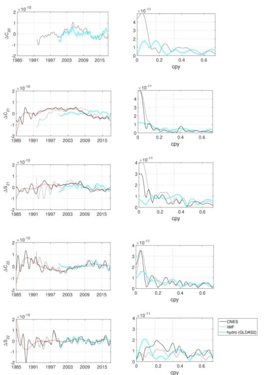
Fig. 5 shows the temporal variation of the Stokes coefficients of degree 2 from SLR obser-vations, along with their amplitude spectra, for both the CNES and IWF solutions. The time-series that are shown have been low-pass filtered with a cut-off period of 1.5 yr to remove the seasonal signals. To highlight longer term variations, we have also applied a low-pass filter with a cut-off period of 8 yr to the CNES solutions (red lines, on Fig. 5). The predicted contribution from hydrological loading products to these Stokes coefficients is also shown on Fig. 5.
3.2.1 Decadal fluctuations
SLR observations show decadal fluctuations (frequencies shorter than ∼ 0.1 cpy) of the order of 4 × 10⁻¹¹. There is a small difference for ∆S21 between CNES and IWF solutions,
probably due to the treatment of the pole tide. Hydrological mass redistribution is important at decadal periods, but current models suggest a limited amplitude of ≈ 2 × 10⁻¹¹, which is too small to explain SLR observations.
3.2.2 Interannual fluctuations
At interannual periods, the CNES and IWF solutions for the coefficients ∆C22 and ∆S22
are reasonably well correlated. Differences between the two SLR solutions are in part due to different processing strategies and differences in the time-window (1984-2017 for CNES vs 1992-2018 for IWF). The longer time period used in the CNES solution introduces nois-ier data, but the spectra in the interannual frequency band nevertheless remain relatively similar. The two different solutions for the coefficients ∆C21 and ∆S21 differ more from one
another – again perhaps as a result of the different treatment of the pole tide – but the amplitude of their fluctuations remain similar. Fluctuations on SLR solutions appear larger prior to ≈ 1996 although this is likely an artifact resulting from the poorer quality of the observations.
The prediction from surface loading contributions has a similar amplitude than the ob-served gravity change recorded by SLR. This is in contrast with the analysis of GPS observa-tions shown in Fig. 3 and 4. Fluctuaobserva-tions in hydrology appear to fit those observed in SLR. In fact, from about 2000 onward, interannual fluctuations in ∆S22, and to a lesser extent
in ∆C22, are reasonably well explained by the hydrological model. The hydrological loading
indicates that the variations are larger at a period around 3 yr. Meyssignac et al. (2013) related such variations on ∆S22to El Ni˜no / Southern Oscillation (ENSO), the Earth’s
dom-inant mode of climate variability on seasonal to interannual time scales. Large fluctuations around 3 yr were also observed in the analyzed GPS series (see Fig. 4).
No clear and distinct periodicity appears to dominate the interannual spectra of the degree-2 gravity field variations. Focusing on periods close to 6 yr, energy peaks are present in the spectra of both ∆S22 and ∆C22, for both the CNES and IWF solutions. Note that
Figure 5. SLR time-series (left) and amplitude spectra (right) corrected for AOD1B non-tidal atmospheric and oceanic effects for the CNES and IWF solutions (1992-2018) for Stokes coefficients (from top to bottom) C20, C21, S21, C22 and S22. The vertical dashed lines on the spectral plots
indicate the location of the 5.9-yr and 3-yr periods. Hydrological (GLDAS2) models are also plotted between 2000 and 2017. The long period trend of the CNES solutions is shown in red and obtained by applying a low-pass filter with a cut-off period 8 yr. The frequency is given in cycle per year (cpy).
the CNES solution. However, it is important to stress that the amplitude of this peak is not significantly higher than the amplitudes of other peaks in the interannual spectra of all coefficients of degree 2.
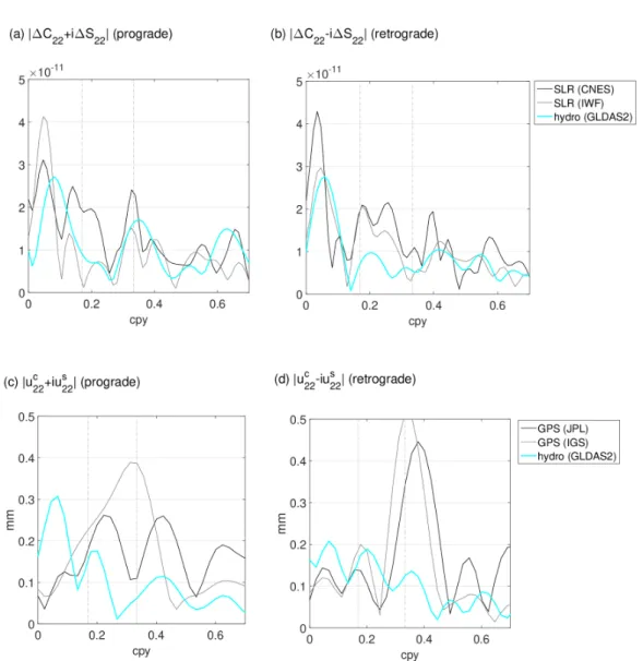
The study of Chao & Yu (2020) reported that the 6 yr variation in ∆C22 and ∆S22 was
further characterized by a coherent westward (retrograde) rotation with an amplitude of 2 × 10⁻¹¹. If this is correct, then the amplitudes of ∆C22and ∆S22 at 6 yr should be similar,
which is approximately the case for the IWF solution on which Chao & Yu (2020) based their analysis. However, it is not the case for the CNES solution, for which the energy peaks in ∆C22 and ∆S22 do not have the same amplitudes and have different offsets from a period
of 6 yr.
To further explore this, we have computed the time series of possible eastward and westward longitudinally propagating gravity signals of degree 2 and order 2. By writing ∆C22 ± i∆S22 = |∆C22+ i∆S22| exp[±iω0t] exp[2iφ], a westward (eastward) propagating
signal has a FFT spectrum with a resonance peak at −ω0 (ω0). By computing the FFT of
these prograde and retrograde signals, we can recover the presence and frequencies of longi-tudinally propagating waves. We perform the same experiment on the vertical displacements coefficients of degree 2 and order 2 and also compute the FFT of prograde (uc
22+ ius22) and
retrograde (uc22− ius
22) waves.
The amplitude spectra are plotted in Fig. 6. We recover a 6-yr retrograde motion of amplitude 2 × 10⁻¹¹ in both the IWF and CNES solutions, confirming the findings of Chao & Yu (2020). However, its amplitude is not significantly larger than that of other peaks in the interannual period range, for either westward or eastward propagating motions. This is especially the case for the CNES solution. A 6-yr retrograde wave is retrieved in both the IGS and JPL solutions of the vertical displacement. However, its amplitude (∼ 0.1-0.2 mm) is much smaller than the ∼ 1 mm amplitude suggested by Ding & Chao (2018). Moreover, this 6-yr signal is weaker than other possible traveling wave signals, notably a large 3-yr retrograde signal. This 3-yr signal is weak in hydrological loading model although it appears clearly in surficial loading models at individual stations spectra (see Fig. A1 and Fig. A2).
Figure 6. Amplitude Fourier spectra of (a) prograde and (b) retrograde degree-2 order-2 Stokes coefficients for the CNES (1992-2017) and IWF (1992-2018) solutions, and for the (c) and (d) GPS degree-2 solutions. The vertical dashed lines indicate the 5.9-yr and 3-yr periods. Hydrological (GLDAS2) model is also plotted. cpy means cycle per year. A 5 10−11 gravity change in (a) or (b) corresponds to a vertical displacement of ∼ 0.3 mm.
The 6-yr retrograde wave has a significant amplitude when GPS vertical displacements are not corrected for non-tidal atmospheric and oceanic loading (see Fig. A5).
3.3 Comparison between SLR and GPS for degree 2
If we assume that all gravity variations at spherical harmonic degree n are induced by changes in surface load density ∆σn(θ, φ), the latter is connected to the Stokes coefficients
by ∆σn(θ, φ) = aρ 3 2n + 1 1 + k0 n n X m=0 (∆CnmYnm,c(θ, φ) + ∆SnmYnm,s(θ, φ)) , (3)
where a = 6371.2 km is the Earth’s reference radius, ρ = 5515 kg m−3 is the Earth’s mean density and kn0 is a loading Love number. The surface load density is also connected to the vertical displacement of degree-n at the surface by
un = 3 ρ 1 2n + 1h 0 n∆σn, (4)
where h0nis a second loading Love number. The spherical harmonic coefficients of the vertical displacements are then directly related to the Stokes coefficients by
(ucnm, usnm) = Rnm ah0n 1 + k0 n (∆Cnm, ∆Snm) , (5) where Rnm = q
(2 − δm,0)(2n + 1)(n−m)!(n+m)! is the normalization factor commonly used in
geodesy with Stokes coefficients. We are chiefly interested in degree n = 2, and we used h02 = −1.00067429 and k20 = −0.30908948. As a reference, a 10−11 variation in Stokes coeffi-cients of degree 2 corresponds to a loading deformation of ≈ 0.1 mm.
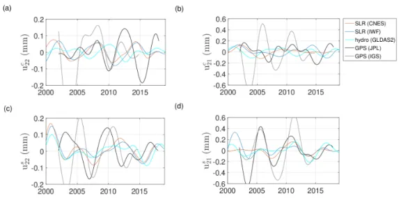
We compare in Fig. 7 the non-zonal degree-2 time-series extracted from GPS solutions, hydrological loading and vertical displacements predicted from SLR Stokes coefficients based on Equation (5). All time-series are band-pass filtered between 4 and 10 yr to focus on interannual periods. The maximum amplitudes at order m = 1 and m = 2 are approximately 0.5 and 0.2 mm, respectively. Note again that the amplitudes of the GPS time-series are typically larger than both the prediction from SLR and the hydrology loading model. Note also that the hydrology model appears to be better correlated with the prediction from SLR than with the observed surface displacements from GPS.
To explore this further, we have computed the correlations between these different time-series. Table 2 shows the correlations for order 1 and Table 3 for order 2. We first analyze the correlation between the different solutions and products for individual coefficients. We then consider cross-correlations and phase shifts between different coefficients.
GPS interannual signals from IGS and JPL solutions are well correlated for uc,s22 and us 21
(64, 67 and 75%), but less so for uc
Figure 7. Median degree-2 time-sequences obtained with the OSE stacking applied on a random distribution of 200 networks of GPS stations for the JPL and IGS solutions corrected for atmo-spheric and oceanic effects using ATMMO products. The observed degree-2 deformation from SLR for both IWF and CNES solutions are also plotted as well as the degree-2 GLDAS2 loading. Time series were band-pass filtered between 4 and 10 yr.
whole consistent with one another. The CNES and IWF solutions from SLR gravity data are also highly correlated (89% and 97% for order-2 and 68% and 77% for order-1), showing that the two different SLR solutions are also consistent with one another. The uc,s22 signal from both SLR solutions is largely correlated with the hydrology loading model (∼ 80%), although a little less so between uc
22 and the CNES solution (60%). The results of Tables 2
and 3 clearly highlight an important hydrological mass contribution to the gravity signal, likely in link with ENSO events for which the impact is mostly on ∆S22 (Meyssignac et al.
2013). The uc
22 signal from both IWF and CNES SLR solutions is correlated at ∼ 70% with uc22
with the JPL GPS solutions and at ∼ 65% with the IGS GPS solutions. The us
22 signal from
IWF SLR solution is more correlated with the GPS solutions (resp. 77 and 58% with JPL and IGS) than the CNES SLR solution (resp. 72 and 54%). A clear correlation (above 70%) shows up on us21 between GLDAS2 hydrological loading and SLR and GPS signals. This is also the case for uc
21, except for the GPS IGS solutions for which the correlation is smaller
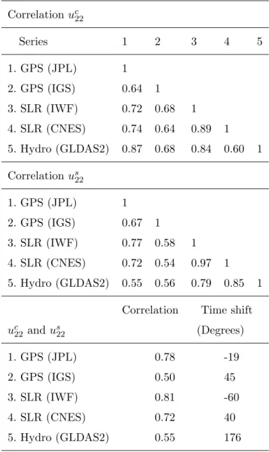
At order-2, the maximum correlation between uc
22 and us22 (∼ 80%) is found from GPS
(JPL solution) and SLR (IWF solution), but with different phase lags (resp. close to -20 and -60 degrees). SLR CNES solution also shows a correlation at most 72% (see Table 3) with a phase lag around -40◦. A strong correlation between uc
22 and us22 with a phase lag of 90
degrees would indicate westward propagating wave, as suggested by Ding & Chao (2018) and Chao & Yu (2020). Table 3 emphasises again that our results do not show strong evidence for such a behavior (see also Fig. 7).
We also witness large correlations between uc21 and us21, in particular for CNES SLR (78%) and to a lesser extent for other solutions, with phase shifts strongly varying from one analysis to the other.
A degree-2 signal coming from a global Earth’s interior process should be characterized by a correlation between GPS and SLR solutions. Our results show that this correlation remains limited, highlighting the present day limits in the resolution of the interannual degree-2 gravity variations and surface deformations. However, the stronger correlation be-tween gravity and hydrology tends to suggest that the degree-2 SLR time-series may be better resolved than the degree-2 GPS time-series. As we noted above, the similar ampli-tudes in the signals from SLR and hydrology models also support this view. The strong correlation between the gravity models and hydrology model and their similar amplitudes also suggest that the observed degree-2 interannual variations are dominantly a signature of surface processes.
We recall that GPS solutions (both JPL and IGS) as well as the IWF SLR solutions are corrected for solid Earth and oceanic pole tides using the same out-of-date mean pole model (from the IERS 2010 Conventions) and not the new conventional linear mean pole model (as in the IERS Conventions updates) used for the CNES SLR solution. The larger discrepancies between solutions of degree-2, order-1 gravity coefficients, is most likely due to this.
Table 2. Maxima of correlation of interannual degree-2 order-1 fluctuations observed from GPS and SLR for different solutions and hydrological loading from GLDAS2 model. Non-tidal atmospheric and oceanic loading have been corrected using ATMMO products for GPS.
Correlation uc21 Series 1 2 3 4 5 1. GPS (JPL) 1 2. GPS (IGS) 0.32 1 3. SLR (IWF) 0.54 0.52 1 4. SLR (CNES) 0.57 0.57 0.68 1 5. Hydro (GLDAS2) 0.66 0.57 0.62 0.75 1 Correlation us21 1. GPS (JPL) 1 2. GPS (IGS) 0.75 1 3. SLR (IWF) 0.61 0.57 1 4. SLR (CNES) 0.63 0.85 0.77 1 5. Hydro (GLDAS2) 0.74 0.79 0.72 0.72 1
Correlation Time shift
uc21 and us21 (Degrees) 1. GPS (JPL) 0.59 -19 2. GPS (IGS) 0.75 44 3. SLR (IWF) 0.55 90 4. SLR (CNES) 0.78 34 5. Hydro (GLDAS2) 0.64 114
4 DISCUSSION: DEGREE-2 GEODETIC OBSERVATIONS: ACCESS TO
EARTH’S INTERIOR PROCESSES?
We have shown that the observed interannual global scale deformation and gravity changes appear to be connected to changes in hydrology at the surface. However, large uncertainties in the observed SLR and GPS signals and in hydrology models prevents us from establishing their connection more strongly. Given this, could there be room for a signal from deeper origin in the observed gravity and surface deformations, for instance from pressure variations
Table 3. Maxima of correlation of interannual degree-2 order-2 fluctuations observed from GPS and SLR for different solutions and hydrological loading from GLDAS2 model. Non-tidal atmospheric and oceanic loading have been corrected using ATMMO products for GPS.
Correlation uc22 Series 1 2 3 4 5 1. GPS (JPL) 1 2. GPS (IGS) 0.64 1 3. SLR (IWF) 0.72 0.68 1 4. SLR (CNES) 0.74 0.64 0.89 1 5. Hydro (GLDAS2) 0.87 0.68 0.84 0.60 1 Correlation us22 1. GPS (JPL) 1 2. GPS (IGS) 0.67 1 3. SLR (IWF) 0.77 0.58 1 4. SLR (CNES) 0.72 0.54 0.97 1 5. Hydro (GLDAS2) 0.55 0.56 0.79 0.85 1
Correlation Time shift
uc22 and us22 (Degrees) 1. GPS (JPL) 0.78 -19 2. GPS (IGS) 0.50 45 3. SLR (IWF) 0.81 -60 4. SLR (CNES) 0.72 40 5. Hydro (GLDAS2) 0.55 176
at the CMB connected to changes in core flows? The degree-2 time-series of GPS and SLR observations can at least place upper bounds on such CMB pressure variations.
This idea was first attempted by Merriam (1988) and revisited by Dumberry & Bloxham (2004), Greff-Lefftz et al. (2004) and Dumberry (2010). Over the 34 years of SLR data, interannual fluctuations are smaller than 2 × 10⁻¹¹. At degree 2, a 10−11time-varying Stokes coefficient requires a CMB pressure change of ∼ 120 Pa (e.g. Dumberry 2010), which would induce a surface deformation of ∼ 0.5 mm. This is indeed comparable with the degree-2
interannual fluctuations observed in the GPS solutions (see Fig. 4 and Fig. 5). However, 120 Pa is a factor 20 to 40 larger than the dynamical pressure changes estimated from interannual core surface flow variations inferred from geomagnetic data (Gillet et al. 2020). Likewise, a 1.7 mm interannual surface deformation at degree-2, as put forward by Ding & Chao (2018), corresponds to a 3.5 × 10⁻¹¹ time-variation in Stokes coefficients and would require an even larger pressure change at the CMB of ∼ 400 Pa. It is thus likely that the difference between degree-2 deformations inferred independently from GPS and SLR data reflects the limit of resolution of these signals on the one hand, and of hydrology loading models on the other hand.
Hence, the 6-yr westward propagating signal of degree 2 identified in Ding & Chao (2018) (which we do not retrieve in our study) and its associated gravity signature as argued in Chao & Yu (2020) is most unlikely to be a signal of core origin. GPS observations at interannual time-scales are at the level of 1 mm at individual stations. This is similar to the 1.7 mm amplitude observed by Ding & Chao (2018), but as we have shown, we do not recover a clear westward propagating degree-2 signal as their study suggests.
Decadal fluctuations in SLR observations as shown in Fig. 5 have an amplitude of ∼ 4×10⁻¹¹ (Fig. 6) at a period ∼ 30 years. At such time-scales, oscillations of the inner
core (because of the density jump at the inner core boundary) may under some scenarios generate a signal of degree 2 order 2 with an amplitude of ∼ 1.5×10⁻¹¹ (Gillet et al. 2020). This is weaker, although not negligible compared with the observed signal from SLR.
5 CONCLUSION
We have shown the limits in the resolution of the large scale degree-2 interannual geodetic signals of surface deformations and gravity field observed by GPS and SLR techniques, re-spectively. We have also shown the limits in the geophysical models used in the processing of these signals. A more systematic study of the consistency between existing surface load-ing models, surface deformation solutions and GRACE/GRACE-FO gravity field solutions could be performed to complete our work. This would however not change our main
con-clusion or, in the worse case, it could reveal even larger inconsistencies. We conclude that at present day, the agreement between GPS and SLR techniques is not sufficiently good to fully characterize the interannual, global scale, vertical deformations of sub-millimetric amplitudes. Hydrological loading models currently available are also not accurate enough to fit geodetic observations and demonstrate their own limits.
We have confirmed the existence of a 6-yr oscillation in GPS solutions at some stations. However, their projection onto a spherical harmonic decomposition does not strongly support that this signal is associated with a degree-2 pattern. A 6-yr periodicity at degree 2, if at all present, is not more prominent in GPS time-series than degree-2 signals at other interannual periods. No clear degree-2 order-2 geographical signal emerges from the GPS time-series at interannual periods, except for some specific configurations of stations. When this is the case, hydrological loading models also tend to exhibit a similar pattern, though with smaller amplitude. A surficial origin for this apparent oscillation is hence to be favoured, with strong network effect. Current global hydrological models are incomplete. Climatological influences from polar ice areas induce interannual global mass redistributions (e.g. Antarctic ice sheet, Horwath et al. 2012; Memin et al. 2015) that should also be carefully investigated.
Strategies and models used in the processing of SLR and GPS solutions include some uncertainties that also limit possible geophysical interpretation at interannual and longer periods. We note that the SLR technique is less sensitive to network effects than a global inversion of stations positions as must be done in the GPS technique. Hence, global models of low-degree surface deformations may be better determined from SLR observations – together with a relation linking the displacements to the Stokes coefficients, as we have done here – than from GPS observations.
We have shown that at interannual and decadal time-scales continental hydrology has a notable influence on surface deformation and gravity field. Geodetic observations together with surficial layer loadings have been widely studied at seasonal time-scales (e.g. Memin et al. 2020). The work presented here is hence a rare analysis at longer periods where we show the influence of hydrological loading also at interannual and decadal time scales.
Based on the observed interannual variations in surface deformations which do not exceed 1 mm, and interannual variations in the Stokes coefficients of gravity which are limited to 2×10⁻¹¹, an upper bound for the interannual pressure change at the CMB that can induce such signals is approximately 100 Pa. Theoretical predictions of the interannual CMB pressure change of degree 2 is limited to approximately 5 Pa (Gillet et al. 2020). This further supports the view that the observed degree-2 interannual changes in surface deformations and gravity are caused by surface processes.
Interpreting GPS displacements and SLR gravity changes in terms of Earth’s deep inte-rior dynamics is challenging and requires that all other effects, including those surficial fluid layers, have been carefully removed. Current models are however not sufficiently accurate for that purpose. Improvements in surface layers modeling is of great importance in order to scrutinize smaller signals that could originate from the Earth’s core.
6 ACKNOWLEDGMENTS
We thank the reviewers H. Dobslaw, R. Gross and the editor R. Holme for their comments on our manuscript. We are grateful to Paul Rebischung for sharing the IGS Repro2 GNSS time-series and Kristel Chanard (IGN) for fruitful discussions on GNSS data analysis. S.R. also thanks Benjamin F. Chao and Hao Ding for useful clarifications and discussions about their work. S.R. acknowledges financial support by the French Centre National d’Etudes Spatiales (CNES) through the TOSCA program. N.G. was partially supported by the French Centre National d’Etudes Spatiales (CNES) for the study of Earth’s core dynamics in the context of the Swarm mission of ESA. M.D is supported by a Discovery grant from NSERC/CRSNG.
7 DATA AVAILABILITY
SLR solutions computed at the Space Research Institute (IWF) of the Austrian Academy of Sciences (AAS) were initially downloaded from http://geodesy.iwf.oeaw.ac.at/d slr monthly.html but are now computed at the Graz University of Technology and are available upon request by the author ([email protected]). CNES SLR solutions can be downloaded from
https://syrte.obspm. fr/∼bizouard/ipercc. IGS time-series are available from http://acc.igs.org/reprocess2.html. JPL residual time-series were downloaded from https://sideshow.jpl.nasa.gov/post/series.html.
Hydrological, non-tidal atmospheric and oceanic loading products are available at http://loading-u.strasbg.fr.
REFERENCES
Abarca del Rio, R., Gambis, D., & Salstein, D., 2000. Interannual signals in length of day and atmospheric angular momentum, in Annales Geophysicae, vol. 18, pp. 347–364, Springer. Adhikari, S. & Ivins, E. R., 2016. Climate-driven polar motion: 2003–2015, Science Advances,
2(4).
Bloßfeld, M., Rudenko, S., Kehm, A., Panafidina, N., M¨uller, H., Angermann, D., Hugentobler, U., & Seitz, M., 2018. Consistent estimation of geodetic parameters from SLR satellite constellation measurements, Journal of Geodesy, 92, 1003–1021.
Bock, Y. & Melgar, D., 2016. Physical applications of GPS geodesy: a review, Reports on Progress in Physics, 79(10), 106801.
Carr`ere, C. & Lyard, F., 2003. Modeling the barotropic response of the global ocean to atmospheric wind and pressure forcing- comparisons with observations, Geophysical Research Letters, 30(6). Carrou, J. P., 1986. Zoom software : Error analysis and accurate orbit restitution at CNES, in Space Dynamics and Celestial Mechanics, pp. 381–398, ed. Bhatnagar, K. B., Springer Nether-lands, Dordrecht.
Chanard, K., Fleitout, L., Calais, E., Rebischung, P., & Avouac, J.-P., 2018. Toward a Global Horizontal and Vertical Elastic Load Deformation Model Derived from GRACE and GNSS Station Position Time Series, Journal of Geophysical Research: Solid Earth, 123(4), 3225–3237. Chao, B. & Yu, Y., 2020. Variation of the equatorial moments of inertia associated with a 6-year
westward rotary motion in the Earth, Earth and Planetary Science Letters, 542, 116316. Chao, B. F., 2017. Dynamics of axial torsional libration under the mantle-inner core gravitational
interaction, Journal of Geophysical Research: Solid Earth, 122, 560–571.
Chao, B. F., Chung, W., Shih, Z., & Hsieh, Y., 2014. Earth’s rotation variations: a wavelet analysis, Terra Nova, 26, 260–264.
Chen, J., Wilson, C., & Tapley, B., 2005. Interannual variability of low-degree gravitational change, 1980-2002, J. of Geodesy, 78, 535–543.
Chen, J., Wilson, C. R., Kuang, W., & Chao, B. F., 2019. Interannual oscillations in Earth Rotation, Journal of Geophysical Research: Solid Earth, 124(12), 13404–13414.
Chen, J. L. & Wilson, C. R., 2005. Hydrological excitations of polar motion, 1993–2002, Geo-physical Journal International , 160(3), 833–839.
Chen, J. L., Wilson, C. R., & Ries, J. C., 2016. Broadband assessment of degree-2 gravitational changes from GRACE and other estimates, 2002-2015, Journal of Geophysical Research: Solid Earth, 121(3), 2112–2128.
Cheng, M. & Ries, J., 2017. The unexpected signal in GRACE estimates of C20, Journal of
Geodesy, 91, 897–914.
Cheng, M., Ries, J. C., & Tapley, B. D., 2011. Variations of the Earth’s figure axis from satellite laser ranging and GRACE, Journal of Geophysical Research: Solid Earth, 116(B1).
Cheng, M., Tapley, B. D., & Ries, J. C., 2013. Deceleration in the Earth’s oblateness, Journal of Geophysical Research: Solid Earth, 118.
Collilieux, X., Altamimi, Z., Coulot, D., Ray, J., & Sillard, P., 2007. Comparison of very long baseline interferometry, GPS, and satellite laser ranging height residuals from ITRF2005 using spectral and correlation methods, Journal of Geophysical Research: Solid Earth, 112(B12). Couhert, A., Bizouard, C., Mercier, F., Chanard, K., Greff, M., & Exertier, P., 2020. Self-consistent
determination of the Earth’s GM, geocenter motion and figure axis orientation, Journal of Geodesy, 94(113).
Cox, C. M. & Chao, B. F., 2002. Detection of a large-scale mass redistribution in the terrestrial system since 1998, Science, 297(5582), 831–833.
Ding, H. & Chao, B. F., 2015. Data stacking methods for isolation of normal-mode singlets of Earth’s free oscillation: Extensions, comparisons, and applications, Journal of Geophysical Research: Solid Earth, 120(7), 5034–5050.
Ding, H. & Chao, B. F., 2018. A 6-year westward rotary motion in the Earth: Detection and possible MICG coupling mechanism, Earth and Planetary Science Letters, 495, 50–55.
Ding, H. & Shen, W.-B., 2013. Search for the Slichter modes based on a new method: Optimal sequence estimation, Journal of Geophysical Research: Solid Earth, 118(9), 5018–5029.
Dobslaw, H., Bergmann-Wolf, I., Dill, R., Poropat, L., Thomas, M., Dahle, C., Esselborn, S., K¨onig, R., & Flechtner, F., 2017. A new high-resolution model of non-tidal atmosphere and ocean mass variability for de-aliasing of satellite gravity observations: AOD1B RL06, Geophysical Journal International , 211(1), 263–269.
Dong, D., Fang, P., Bock, Y., Cheng, M. K., & Miyazaki, S., 2002. Anatomy of apparent seasonal variations from GPS-derived site position time series, Journal of Geophysical Research: Solid Earth, 107(B4), ETG 9–1–ETG 9–16.
Dumberry, M., 2010. Gravity variations induced by core flows, Geophysical Journal International , 180(2), 635–650.
Dumberry, M. & Bloxham, J., 2004. Variations in the Earth’s gravity field caused by torsional oscillations in the core, Geophysical Journal International , 159(2), 417–434.
Fang, M., Hager, B. H., & Herring, T. A., 1996. Surface deformation caused by pressure changes in the fluid core, Geophysical Research Letters, 23(12), 1493–1496.
Fu, Y., Freymueller, J., & Jensen, T., 2012. Seasonal hydrological loading in southern Alaska observed with GPS and GRACE, Geophysical Research Letters, 39(15)(15310).
G´egout, P., Boy, J.-P., Hinderer, J., & Ferhat, G., 2010. Modeling and observation of loading contribution to time-variable GPS sites positions, in Gravity, geoid and Earth observation, pp. 651–659, Springer.
Gelaro, R., McCarty, W., Su´arez, M. J., Todling, R., Molod, A., Takacs, L., Randles, C. A., Darmenov, A., Bosilovich, M. G., Reichle, R., et al., 2017. The modern-era retrospective analysis for research and applications, version 2 (MERRA-2), Journal of Climate, 30(14), 5419–5454. Gillet, N., Jault, D., Canet, E., & Fournier, A., 2010. Fast torsional waves and strong magnetic
field within the Earth’s core, Nature, 465(7294), 74–77.
Gillet, N., Huder, L., & Aubert, J., 2019. A reduced stochastic model of core surface dynamics based on geodynamo simulations, Geophysical Journal International , 219(1), 522–539.
Gillet, N., Dumberry, M., & Rosat, S., 2020. The limited contribution from outer core dynamics to global deformations at the Earth’s surface, Geophysical Journal International , 224, 216–229. Greff-Lefftz, M., Pais, M., & Le Mou¨el, J.-L., 2004. Surface gravitational field and topography
changes induced by the Earth’s fluid core motions, Journal of Geodesy, 78(6), 386–392.
Heflin, M., Donnellan, A., Parker, J., Lyzenga, G., Moore, A., Ludwig, L. G., Rundle, J., Wang, J., & Pierce, M., 2020. Automated Estimation and Tools to Extract Positions, Velocities, Breaks, and Seasonal Terms From Daily GNSS Measurements: Illuminating Nonlinear Salton Trough Deformation, Earth and Space Science, 7(7), e2019EA000644.
Holme, R. & De Viron, O., 2013. Characterization and implications of intradecadal variations in length of day, Nature, 499, 202–204.
Horwath, M., Legr´esy, B., R´emy, F., Blarel, F., & Lemoine, J., 2012. Consistent patterns of Antarctic ice sheet interannual variations from ENVISAT radar altimetry and GRACE satellite gravimetry, Geophysical Journal International , 189(2), 863–876.
IERS Conventions, 2010. IERS Technical note 36, p. 179, eds Petit, G. & Luzum, B., Frankfurt am Main: Verlag des Bundesamts f¨ur Kartographie und Geod¨asie.
Jungclaus, J. H., Fischer, N., Haak, H., Lohmann, K., Marotzke, J., Matei, D., Mikolajewicz, U., Notz, D., & von Storch, J. S., 2013. Characteristics of the ocean simulations in the Max Planck Institute Ocean Model (MPIOM) the ocean component of the MPI-Earth system model, Journal of Advances in Modeling Earth Systems, 5(2), 422–446.
Kusche, J. & Schrama, E. J. O., 2005. Surface mass redistribution inversion from global GPS deformation and Gravity Recovery and Climate Experiment (GRACE) gravity data, Journal of Geophysical Research: Solid Earth, 110(B9).
Larson, K. M., 2019. Unanticipated Uses of the Global Positioning System, Annual Review of Earth and Planetary Sciences, 47, 19–40.
Loomis, B. D., Rachlin, K. E., & Luthcke, S. B., 2019. Improved Earth Oblateness Rate Re-veals Increased Ice Sheet Losses and Mass-Driven Sea Level Rise, Geophysical Research Letters, 46(12), 6910–6917.
Lyard, F., Lef`evre, F., Letellier, T., & Francis, O., 2006. Modeling the global ocean tides: A modern insight from FES2004, Ocean Dynamics, 56, 394–415.
Maier, A., Krauss, S., Hausleitner, W., & Baur, O., 2012. Contribution of satellite laser ranging to combined gravity field models, Advances in Space Research, 49, 556–565.
Memin, A., Flament, T., Alizier, B., Watson, C., & R´emy, F., 2015. Interannual variation of the Antarctic Ice Sheet from a combined analysis of satellite gravimetry and altimetry data, Earth and Planetary Science Letters, 422, 150–156.
Memin, A., Boy, J.-P., & Santamaria-Gomez, A., 2020. Correcting GPS measurements for non-tidal loading, GPS Solutions, 24(45).
Merriam, J., 1988. Limits on lateral pressure gradients in the outer core from geodetic observa-tions, Physics of the Earth and Planetary Interiors, 50, 280–290.
Meyssignac, B., Lemoine, J. M., Cheng, M., Cazenave, A., G´egout, P., & Maisongrande, P., 2013. Interannual variations in degree-2 Earth’s gravity coefficients C2,0, C2,2, and S2,2 reveal large-scale mass transfers of climatic origin, Geophysical Research Letters, 40, 1–6.
Nahmani, S., Bock, O., Bouin, M.-N., Santamar´ıa-G´omez, A., Boy, J.-P., Collilieux, X., M´etivier, L., Panet, I., Genthon, P., de Linage, C., & W¨oppelmann, G., 2012. Hydrological deformation in-duced by the West African Monsoon: Comparison of GPS, GRACE and loading models, Journal of Geophysical Research: Solid Earth, 117(B5).
Nerem, R. S. & Wahr, J., 2011. Recent changes in the Earth’s oblateness driven by Greenland and Antarctic ice mass loss, Geophysical Research Letters, 38(13).
Petrov, L. & Boy, J.-P., 2004. Study of the atmospheric pressure loading signal in VLBI observa-tions, Journal of Geophysical Research, 109(B03405).
Picot, N., Marechal, C., Couhert, A., Desai, S., Scharroo, R., & Egido, A., 2018. Jason-3 products handbook, 1(5), 28–31.
Ray, R., 1999. A global ocean tide model from topex/poseidonaltimetry: GOT 99.2, NASA Technical Memorandum, 209478, 58 pages.
Journal of Geodesy, 90, 611–630.
Rodell, M., Houser, P., Jambor, U., Gottschalck, J., Mitchell, K., Meng, C.-J., Arsenault, K., Cosgrove, B., Radakovich, J., Bosilovich, M., et al., 2004. The global land data assimilation system, Bulletin of the American Meteorological Society, 85(3), 381–394.
Santamar´ıa-G´omez, A. & Ray, J. R., 2020. Chameleonic noise in GPS position time series, Earth and Space Science Open Archive, p. 26.
Tapley, B. D., Bettadpur, S., Watkins, M., & Reigber, C., 2004. The gravity recovery and climate experiment: Mission overview and early results, Geophysical Research Letters, 31(9).
Tapley, B. D., Watkins, M., & Flechtner, F. e. a., 2019. Contributions of GRACE to understanding climate change, Nature Climate Change, 9, 358–369.
van Dam, T., Wahr, J., Milley, C., Shmakin, A., Blewitt, G., & et al., 2001. Crustal displacements due to continental water loading, Geophysical Research Letters, 28(651), 54.
Watkins, A., Fu, Y., & Gross, R., 2018. Earth’s subdecadal angular momentum balance from deformation and rotation data, Scientific reports, 8(1), 13761.
Welch, P. D., 1967. The use of Fast Fourier Transform for the estimation of power spectra: A method based on time averaging over short, modified periodograms, IEEE Transactions on Audio and Electroacoustics, AU-15(2), 70–73.
Wunsch, C., Heimbach, P., Ponte, R., Fukumori, I., & the ECCO-GODAE Consortium Mem-bers, 2009. The global general circulation of the ocean estimated by the ECCO-consortium, Oceanography, 22(2), 88–103.
Zou, R., Wang, Q., Freymueller, J., Poutanen, M., & Cao, X., 2015. Seasonal hydrological loading in Southern Tibet detected by joint analysis of GPS and GRACE, Sensors, 15(30525), 38.
APPENDIX A: GPS INDIVIDUAL TIME-SERIES AND AMPLITUDE SPECTRA
We show in Fig. A1 and Fig. A2 the spectral amplitudes and in Fig. A3 and Fig. A4 the time-series of JPL and IGS GPS solutions at the selected stations identified in Fig. 1. Hydrological loading and its sum with non-tidal atmospheric and oceanic loadings are also plotted.
At some sites a spectral peak around 6 years is clear, with an amplitude up to about 1.5 mm (e.g. CEDU, HRAO, KERG, PERT, SANT, TIBB), while it is absent at other sites (e.g. GLSV, TIXI, VILL, ZIMM). In many places peaks of millimetric magnitude are also seen at both longer and shorter periods within the interannual range. In particular, a 3-yr signal
appears at many sites (e.g. AREQ, BOR1, CAS1, CHUR, COCO, DARW, GOLD, HNPT, JOZE, KARR, KERG, KIRU, MCM4, MDO1, NLIB, PERT, REYK, TIXI, TMGO, TWO2, TSKB, WILL, YAR2, ZIMM) with an amplitude sometimes as large as or even larger than the 6-yr signal.
The amplitude of the hydrological contribution is on average smaller than the observed 6-yr signal at most GPS sites, with an amplitude up to about 1 mm. Besides hydrology, non-tidal atmospheric loading and oceanic response to the wind and atmospheric forcings also contribute to GPS observations with smaller amplitudes (see Fig. A1 and Fig. A2).
At a few sites (e.g. AREQ, DOUR, HOBU, JOZE, ZECK), hydrological loading also shows some spectral energy around 6 yr for both MERRA2 and GLDAS2 products, which are then candidates to partly explain the observed spectral line. At some sites (e.g. ALGO, GOPE, POL2, QUIN, ZECK) non-tidal atmospheric and oceanic loading slightly improves the fit between the surficial loading and GPS observation since the vertical displacement around 6 yr matches the predicted total surficial loading (sum of non-tidal atmospheric, oceanic and hydrological loading). At other sites, amplitude or frequency is slightly different (e.g. BOR1, BRIB, CHUM, DOUR, JOZE, MAWY, WILL, DRAO, GOLD, GRAS, GRAZ, HERS, MAS1, MONP, SFER, WILL) or surficial loading models show too little power at 6 yr to fit the observed GPS signal (e.g. CEDU, HRAO, PERT, SANT, TIBB). Similar observations can be done with the IGS solutions and at the 3-yr period. The stations that feature a large 6-yr or 3-yr peak are localized in very different geographical context in terms of proximity to the oceans, hydrology, and whether they are on continents or on islands.
When investigating the time-series, we can see a rather good fit in terms of amplitude and phase between the surficial loading and the GPS observations at several sites (e.g. ALGO, ALIC, BOR1, GOPE, GRAZ, PIE1, SFER, SYOG, ZECK), despite some discrepancies attributed to raw data offset processing.
Figure A1. Amplitude spectra of the JPL time-series (black) and surficial loading at the 83 stations of Fig. 1a. MERRA2 (in dark blue) and GLDAS2 (in blue) hydrological loadings are plotted. Sums of non-tidal atmospheric and oceanic with hydrological contributions are also plotted in orange (ATMMO+MERRA2) and brown (ATMIB+ECCO2+GLDAS2). The vertical dash-dotted lines indicate the 5.9-yr and 3-yr periods. Common time-span of the series is January 2002 - December 2017. cpy means cycle per year.
Figure A2. Amplitude spectra of the IGS time-series (black) and surficial loading at the 63 stations of Fig. 1b. MERRA2 (in dark blue) and GLDAS2 (in blue) hydrological loadings are plotted. Sums of non-tidal atmospheric and oceanic with hydrological contributions are also plotted in orange (ATMMO+MERRA2) and brown (ATMIB+ECCO2+GLDAS2). The vertical dash-dotted line indicate the 5.9-yr and 3-yr periods. Common time-span of the series is January 2002 - October 2014. cpy means cycle per year.
APPENDIX B: OPTIMAL SEQUENCE ESTIMATE
The so-called Optimal Sequence Estimate (OSE) was originally proposed by Ding & Shen (2013) in the search for the degree-1 translational oscillation of the solid inner-core. This method was thoroughly tested against possible variant spherical harmonic stacking methods by Ding & Chao (2015) for the analysis of seismic modes. This OSE method corresponds indeed to a generalized inverse problem where we want to find the spherical harmonic com-ponents for a target degree-l signal from a distributed network of N stations.
Denoting ui the time-varying signal (e.g. surface displacement or gravity change) at a
station i of colatitude θi and longitude φi, we assume that this observation contains the
Figure A3. Time-series of the JPL solutions (black) and surficial loadings at the 83 stations of Fig. 1a band-pass filtered between 4 and 10 years. MERRA2 (in dark blue) and GLDAS2 (in blue) hydrological loadings are plotted. Sums of non-tidal atmospheric and oceanic with hydrological contributions are also plotted in orange (ATMMO+MERRA2) and brown (AT-MIB+ECCO2+GLDAS2).
Figure A4. Time-series of the IGS solutions (black) and surficial loadings at the 63 stations of Fig. 1b band-pass filtered between 4 and 10 years. MERRA2 (in dark blue) and GLDAS2 (in blue) hydrological loadings are plotted. Sums of non-tidal atmospheric and oceanic with hydrological contributions are also plotted in orange (ATMMO+MERRA2) and brown (AT-MIB+ECCO2+GLDAS2).
complex fully-normalized harmonic functions Ym
n , we write
U (t) = Y A(t), (B.1)
where U (t) = [u1(t) u2(t) ... uN(t)] is the matrix of the time-series and
Y = Yn−n(θ1, φ1) Yn−n+1(θ1, φ1) ... Ynn(θ1, φ1) Yn−n(θ2, φ2) Yn−n+1(θ2, φ2) ... Ynn(θ2, φ2) .. . ... ... ... Yn−n(θN, φN) Yn−n+1(θN, φN) ... Ynn(θN, φN) (B.2)
is the matrix of the complex spherical harmonics functions evaluated at the N stations. The (2n + 1)-vector A is the general least-squares solution of Eq. (B.1)
Figure A5. Amplitude Fourier spectra of (a) prograde and (b) retrograde degree-2 order-2 GPS vertical displacements for which non-tidal atmospheric and oceanic loading has not been subtracted. Hydrological (MERRA2) model is also plotted. cpy means cycle per year.
where T denotes the transpose of the matrix and W is a diagonal weighting matrix. W
can be constructed from the standard deviation of the N time-series for instance. In our application of the OSE, we did not assign any weight, so W is the identity matrix.
APPENDIX C: INFLUENCE OF THE NON-TIDAL ATMOSPHERIC AND OCEANIC LOADING ON DEGREE-2 INTERANNUAL GPS VERTICAL DISPLACEMENT
In the analysis presented in the main text, the GPS vertical displacements have been cor-rected for the non-tidal atmospheric and oceanic loading. When this effect is not subtracted from GPS solutions, the spectral amplitudes of the prograde and retrograde degree-2 order-2 GPS displacements show a 6-yr retrograde signal nearly as large as the 3-yr retrograde one (Fig. A5). We must then favor the influence of surficial loading over a core origin as a possible explanation for this 6-yr retrograde wave.