Solar cycle variations of stratospheric ozone and temperature in simulations of a coupled chemistry-climate model
Texte intégral
Figure


Documents relatifs
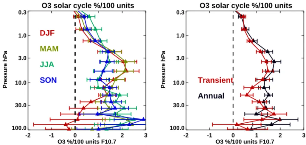
The simulations reproduce this main latitudinal structure of the observed ozone trend, with small trends in the tropics and high trends at high latitudes. The seasonal variation
The input data bias between these two experiments produces only a small difference in the ozone analyses for GOATS runs with chemistry (Fig.. Title Page Abstract
Left Panel: As in Figures 1 and 2, but composites of all the model results which forced a solar cycle in both the radiative heating and photolysis rates (upper panels) and those
Correlation plots of ozone return dates against Cl y return dates for (a, c, e) the Antarctic and (b, d, f) the Arctic from REF-C2 simulations for individual models and the MMM1S at
ozone metrics in the TOAR database. The metrics relevant to climate and global atmospheric chemistry model evalu- ation that were selected for TOAR-Climate are: 1) the sea-
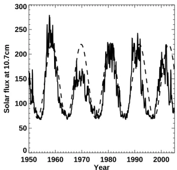
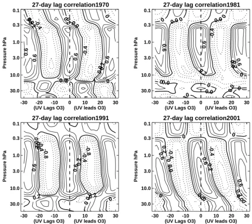
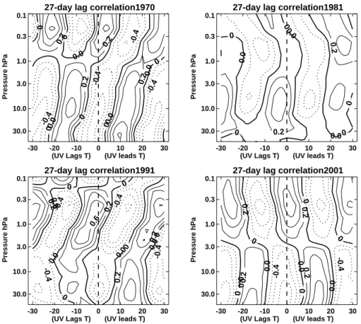
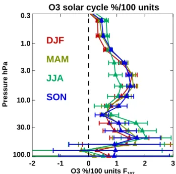
Recent observational studies using ground-based and satellite data sets agree with previous results, re- porting ozone variations in phase with the 11-year and 27-day solar cycle
Changes in atmospheric chemistry, which are due to solar flux variations, must be explained by solar activity effects in the spectral ranges of the 0
Correlation plots of ozone return dates against Cl y return dates for (a, c, e) the Antarctic and (b, d, f) the Arctic from REF-C2 simulations for individual models and the MMM1S at
