Climate model boundary conditions for four Cretaceous time slices

(1)

HAL Id: hal-00298187

https://hal.archives-ouvertes.fr/hal-00298187

Submitted on 4 Jun 2007

HAL is a multi-disciplinary open access

archive for the deposit and dissemination of sci-entific research documents, whether they are pub-lished or not. The documents may come from teaching and research institutions in France or abroad, or from public or private research centers.

L’archive ouverte pluridisciplinaire HAL, est destinée au dépôt et à la diffusion de documents scientifiques de niveau recherche, publiés ou non, émanant des établissements d’enseignement et de recherche français ou étrangers, des laboratoires publics ou privés.

Climate model boundary conditions for four Cretaceous

time slices

J. O. Sewall, R. S. W. van de Wal, K. van der Zwan, C. van Ooosterhout, H.

A. Dijkstra, C. R. Scotese

To cite this version:

J. O. Sewall, R. S. W. van de Wal, K. van der Zwan, C. van Ooosterhout, H. A. Dijkstra, et al.. Climate model boundary conditions for four Cretaceous time slices. Climate of the Past Discussions, European Geosciences Union (EGU), 2007, 3 (3), pp.791-810. �hal-00298187�

(2)

CPD

3, 791–810, 2007 Cretaceous boundary conditions J. O. Sewall et al. Title Page Abstract Introduction Conclusions References Tables Figures ◭ ◮ ◭ ◮ Back Close Full Screen / Esc

Printer-friendly Version Interactive Discussion

EGU

Clim. Past Discuss., 3, 791–810, 2007 www.clim-past-discuss.net/3/791/2007/ © Author(s) 2007. This work is licensed under a Creative Commons License.

Climate of the Past Discussions

Climate of the Past Discussions is the access reviewed discussion forum of Climate of the Past

Climate model boundary conditions for

four Cretaceous time slices

J. O. Sewall1,*, R. S. W. van de Wal1, K. van der Zwan2, C. van Ooosterhout3, H. A. Dijkstra1, and C. R. Scotese4

1

Institute for Marine and Atmospheric Research, Utrecht University, Princetonplein 5, 3584 CC Utrecht, The Netherlands

2

Faculty of Geosciences, P.O. Box 80021, 3508 TA Utrecht, The Netherlands

3

Shell International Exploration and Production, P.O. Bos 60, 2280 Rijswijk, The Netherlands

4

PALEOMAP Project, Department of Earth and Environmental Sciences, University of Texas at Arlington, Texas, 76019, USA

*

now at: Department of Geosciences, Virgina Tech, 4044 Derring Hall (0420) Blacksburg, VA 24061, USA

Received: 14 May 2007 – Accepted: 14 May 2007 – Published: 4 June 2007 Correspondence to: J. O. Sewall (j.sewall@phys.uu.nl)

(3)

CPD

EGU Abstract

General circulation models (GCMs) are useful tools for investigating the characteristics and dynamics of past climates. Understanding of past climates contributes significantly to our overall understanding of Earth’s climate system. One of the most time con-suming, and often daunting, tasks facing the paleoclimate modeler, particularly those

5

without a geological background, is the production of surface boundary conditions for past time periods. These boundary conditions consist of, at a minimum, continen-tal configurations derived from plate tectonic modeling, topography, bathymetry, and a vegetation distribution. Typically, each researcher develops a unique set of boundary conditions for use in their simulations. Thus, unlike simulations of modern climate,

10

basic assumptions in paleo surface boundary conditions can vary from researcher to researcher. This makes comparisons between results from multiple researchers difficult and, thus, hinders the integration of studies across the broader community. Unless special changes to surface conditions are warranted, researcher dependent boundary conditions are not the most efficient way to proceed in paleoclimate

inves-15

tigations. Here we present surface boundary conditions (land-sea distribution, pale-otopography, paleobathymetry, and paleovegetation distribution) for four Cretaceous time slices (120 Ma, 110 Ma, 90 Ma, and 70 Ma). These boundary conditions are modified from base datasets to be appropriate for incorporation into numerical stud-ies of Earth’s climate and are available in NetCDF format upon request from the lead

20

author. The land-sea distribution, bathymetry, and topography are based on the 1◦ ×1◦ (latitude x longitude) paleo Digital Elevation Models (paleoDEMs) of Christopher Scotese. Those paleoDEMs were adjusted using the paleogeographical reconstruc-tions of Ronald Blakey (Northern Arizona University) and published literature and were then modified for use in GCMs. The paleovegetation distribution is based on published

25

data and reconstructions and consultation with members of the paleobotanical com-munity and is represented as generalized biomes that should be easily translatable to many vegetation-modeling schemes.

(4)

CPD

EGU 1 Introduction

Over the last few decades, the use of numerical models to investigate Earth’s climate history has increased (e.g. Barron, 1984; Sloan and Barron, 1992; Huber and Sloan, 2001; Otto-Bliesner et al., 2002; DeConto and Pollard, 2003; Sewall and Sloan, 2006). As those models have grown in sophistication, resolution, and complexity, the level of

5

informational input that they require has also grown. At the most basic level, all Gen-eral Circulation Models (GCMs) run on a representation of the physical Earth. Basic geography, elevation, and bathymetry must be defined. In addition, in many models (e.g. ECHAM5, CCSM3; Jungclaus et al., 2005; Collins et al., 2006) the characteristics of the land surface (soil conditions, vegetation distribution, locations of land ice, river

10

runoff paths etc.) must also be defined. While all of these quantities are relatively easy to obtain for the present day, researchers simulating paleoclimates can face a daunting and time consuming task when developing surface boundary conditions.

The production of such boundary conditions frequently involves a comprehensive search of the literature for published estimates of elevations, ocean depths, continental

15

locations, and vegetation types in a specific time period. These, often limited, data points are then integrated with general, regional geological and biological information to build a suite of boundary conditions from scratch. This time consuming task is of-ten completed by researchers with geological and paleontological training. However, as more and more researchers focus on understanding Earth’s climate history through

nu-20

merical modeling, an increasing proportion of those researchers have backgrounds in other, equally important, disciplines (e.g. Dynamic Meteorology, Physics, Atmospheric Dynamics, Physical Oceanography), and for those researchers, generating appropri-ately detailed boundary conditions for a given time in Earth’s history can be a non-trivial task. In addition, while sensitivity studies investigating the influence of changing

sur-25

face conditions on climate are an integral part of understanding climatic conditions in the past, many paleoclimate investigations would benefit from a common set of surface boundary conditions. Such common boundary conditions would permit clearer

(5)

com-CPD

EGU

parisons between work from multiple research groups and would encourage greater ease and progress toward integrating a community-wide understanding of the climate system in a given time period.

To this end, we present climate model boundary conditions for four Cretaceous time slices generated as part of a study focused on understanding the dynamics and history

5

of the Cretaceous oceans. Those time slices are: the early Aptian (∼120 Ma±5 Ma), the early Albian (∼110 Ma±5 Ma), the Cenomanian/Turonian boundary (∼90 Ma±5 Ma) and the early Maastrichtian (∼70 Ma±5 Ma); an excellent description of the concept of a time slice can be found in Markwick and Valdes (2004). We present the essence of our geographical, topographic, and vegetative boundary conditions in this paper, and the

10

boundary condition files are available upon request. In disseminating these boundary conditions, it is our intent to aid other researchers interested in investigating Creta-ceous climates and, thus, facilitate a greater and more rapid understanding of some of the outstanding and integral questions in the dynamics of greenhouse climates.

2 Methods

15

We begin creating our Cretaceous boundary conditions with the global geography, to-pography, and bathymetry for each time slice. We alter these base datasets to incor-porate new information and to render them appropriate for use in GCMs. On top of this physical surface, we then layer the appropriate land surface by including land ice, veg-etation, surface runoff paths, and soil conditions. The base datasets for global

geogra-20

phy, topography, and bathymetry for all four of our Cretaceous time slices were obtained from the PALEOMAP project’s set of 50 Phanerozoic, 1◦ latitude × 1◦ longitude, paleo Digital Elevation Models (paleoDEMS); in some instances, the paleoDEMs were modi-fied based on published literature and the paleogeographical reconstructions of Ronald Blakey (http://jan.ucc.nau.edu/$\sim$rcb7/globaltext2.html). From this basis, datasets

25

were first converted into NetCDF format and interpolated to a resolution of ∼2.8◦ lati-tude × 2.8◦longitude (∼280 km×280 km) using the NCAR Command Language (NCL;

(6)

CPD

EGU http://www.ncl.ucar.edu/). The NetCDF datasets were then manipulated using

MAT-LAB with MEXNC and the NetCDF Toolbox installed (http://mexcdf.sourceforge.net/). Modifications to the original datasets included merging differing paleogeographical or topographical elements and altering the geography, topography and bathymetry such that they can easily be incorporated as the lower boundary condition of a GCM. Such

5

alterations include the removal of marginal seas (ocean areas with limited or no con-nection to the global ocean), the expansion of narrow ocean gateways to allow unre-stricted flow, the merging of island clusters without sufficient flow between islands, and the removal of most areas of internal drainage on continents. While features such as these may be realistic aspects of the paleogeography/topography, they pose

numer-10

ical problems for GCMs (e.g. Wajsowicz, 1995, 1996) and must be removed in the production of functional boundary conditions. In addition, the relatively coarse spatial resolution of GCMs prohibits the resolution of geographical details and, consequently, model boundary conditions must always be a smoothed approximation of the actual paleo land surface.

15

In all time slices, the most extensive modifications made to the paleogeographic reconstructions were in the geographically complex regions of western Eurasia, Tethys, the South Atlantic, and the South Polar region. In all instances, the complexity of the geography was reduced to create fewer landmasses and larger, better-defined ocean regions to allow for more accurate numerical modeling of the global earth system.

20

In individual time slices, we made time or geographically specific changes to render geography and elevation compatible with GCM requirements and we also made spe-cific choices in regions where the paleogeography/topography is debatable between various researchers. Those specific changes and choices are detailed here.

In the Aptian, we created a south polar land mass (absent in the paleogeographical

25

reconstruction) to avoid the pole problem in ocean models (we note here that all ge-ographies are constructed assuming a single pole in the Southern Hemisphere and the ability to move the north pole to Greenland or generate a tripolar grid with one North-ern Hemisphere pole in Eurasia and one in North America). While the reconstructions

(7)

CPD

EGU

of Blakey (http://jan.ucc.nau.edu/∼_{rcb7/globaltext2.html}_{), Meschede and Frisch (1998),}

and Ross and Scotese (1988) indicate islands in the Panama Strait at this time, more recent reconstructions by Scotese (http://www.scotese.com; Scotese, 2001) do not. Primarily because islands are computationally expensive and limit, if not prohibit, flow through this narrow gateway, we choose to exclude them from our boundary

condi-5

tions. The reconstructions of Blakey and Scotese also disagree on the presence of a Cretaceous Interior Seaway in Western North America in the early Aptian. As a partial seaway is undoubtedly present in the Albian and a full seaway present at the Cenoma-nian/Turonian boundary, we opt to exclude the Western North American Cretaceous Interior Seaway from our Aptian boundary conditions such that our boundary

condi-10

tions through the Early Cretaceous represent a suite of possible seaway configurations (no seaway in the early Aptian, a partial seaway in the early Albian, and an extensive seaway at the Cenomanian/Turonian boundary); this is done in order to capture the sensitivity of modeled flow to changing geographical conditions.

In the Albian, the reconstructions of Blakey (http://jan.ucc.nau.edu/∼_{rcb7/globaltext2.}

15

html) again indicate islands in the Panama Strait, those of Scotese (http://www.scotese.

com; Scotese, 2001) do not. Due to the computational expense and potential for in-hibiting flow, we again choose to exclude these islands from our boundary conditions. The reconstructions of Blakey and Scotese also disagree on the extent of the Creta-ceous Interior Seaway of Western North American and the presence of a sea strait to

20

the immediate west of Greenland. As the seaway extent proposed by Blakey in the Albian is similar to that proposed by both researchers for the Cenomanian/Turonian boundary, we opt for a limited Western North American Cretaceous Interior Seaway, similar to that proposed by Scotese, such that our boundary conditions over the Early Cretaceous continue to represent a suite of possible seaway configurations.

Further-25

more, as Dam et al. (1998) indicate that a sea strait west of Greenland only came into being during the Cenomanian/Turonian, we also exclude this feature from our Albian boundary conditions. While all paleogeographic reconstructions indicate that South America and Africa have fully separated by the early Albian, the sea strait between

(8)

CPD

EGU

them is represented as shallow and narrow enough that flow in the strait was unlikely to be significant and is not readily resolvable at our horizontal resolution (∼2.8◦latitude × 2.8◦longitude). Consequently, and to ensure that our boundary conditions represent a suite of South Atlantic opening stages (closed in the Aptian, closed but with an ex-tensive embayment in the Albian, open in a narrow strait at the Cenomanian/Turonian

5

boundary, and fully open in the Maastrichtian), we connect northwestern Africa and northeastern South America in our Albian boundary conditions.

At the Cenomanian/Turonian boundary, the Cretaceous Interior Seaway of West-ern North America is open in our boundary conditions and, based on the presence of Marine Cenomanian/Turonian strata west of Greenland (Dam et al., 1998), we opt to

10

reduce the elevation of western Greenland and emplace a seaway just west of Green-land. While the reconstructions of Blakey (http://jan.ucc.nau.edu/∼_{rcb7/globaltext2.}

html), Scotese (http://www.scotese.com; Scotese, 2001), Meschede and Frisch (1998), and Ross and Scotese (1988) all indicate the presence of small islands in the Panama Strait, those islands would limit, if not inhibit, flow through the strait, which was

decid-15

edly open, thus, we remove those islands in our boundary conditions.

In the earliest Maastrichtian, the reconstructions of Blakey (http://jan.ucc.nau.edu/

∼_{rcb7/globaltext2.html) and Scotese (}_{http://www.scotese.com}_{; Scotese, 2001) again} disagree on the presence of a Western North American Cretaceous Interior Seaway. However, the seaway presented by Blakey is extremely narrow and flow in and out

20

of it was unlikely to have a significant influence on the Arctic Ocean (its only connec-tion) and is not resolvable at our horizontal resolution, thus, we have not represented a Western North American Cretaceous Interior Seaway in our Maastrichtian boundary conditions. The above argument is also true for the South American Interior Seaway just east of the Andes, which is included in our Cenomanian/Turonian boundary

condi-25

tions but excluded from our Maastrichtian boundary conditions. The reconstructions of both Blakey and Scotese suggest an open Tasman strait in the Maastrichtian, however, the initial report of ODP Leg 189 (Exon et al., 2001) indicates a narrow, shallow, island choked connection, which was unlikely to transmit significant flow, and opening it to a

(9)

CPD

EGU

width and depth resolvable at our horizontal resolution would likely result in an over-prediction of flow through this strait. Consequently, we have a closed Tasman Strait in our Maastrichtian boundary conditions.

Global vegetation distributions for each of the four time slices were created in MAT-LAB by hand and are based on published paleobotanical data (Spicer and Chapman,

5

1990; Vakhrameev, 1991; Saward, 1992; Mohr and Lazarus, 1994; Otto-Bliesner and Upchurch, 1997; Archangelsky, 2001; Spicer and Herman, 2001; Mohr and Rydin, 2002; Spicer et al., 2002; van Waveren et al., 2002; Archangelsky, 2003). The vege-tation types used have been generalized from those of the NCAR Land Surface Model (Bonan, 1998) in an effort to make them broadly applicable to both our degree of

un-10

derstanding of Cretaceous vegetation distributions and the varying vegetation schemes employed in different land surface models. Given the limited data on Early Cretaceous global vegetation distributions and the significant evolutionary changes in plants during that epoch (Crane et al., 2002), we specify vegetation in functional biomes – groupings of plants that, regardless of biology, probably had the same community structure and

15

climate influence. In addition, those biomes were created to be as general and in-clusive as possible while still maintaining significant differences (from a climatological point of view) between different biomes. The ten biomes represented in our vegeta-tion scheme are: High altitude/latitude, evergreen, conifer, closed canopy forest; High altitude/latitude mixed forest with equal percentage of broad and needle leaved and

ev-20

ergreen and deciduous trees; Low altitude/latitude, evergreen, conifer, closed canopy forest; Closed canopy, broad leaved, moist, evergreen forest; Closed canopy, broad leaved, dry, deciduous forest; Savanna (dry, low understory with sparse, broad leaved overstory); High altitude/latitude, moist, open canopy, evergreen forest with a shrub understory; Low altitude/latitude, moist, open canopy, mixed evergreen/deciduous,

for-25

est with a shrub understory; Wet or cool evergreen shrubland; Dry or warm deciduous shrubland. After entering published data points or reconstructions into MATLAB, the vegetation type was altered to match one of the available types in our scheme. The areas between published tie points were filled based on expected, large-scale climate

(10)

CPD

EGU

patterns, published reconstructions (Vakhrameev, 1991; Saward 1992; Otto-Bliesner and Upchurch, 1997), and interpolation between related data points. The completed paleovegetation distributions were then distributed to members of the paleobotanical community for consultation and presented at an international conference for comment (Dijkstra and Sewall, 2006). Expert commentary was then integrated into the final

5

paleovegetation distribution.

3 Boundary conditions

The boundary conditions for each of the four time slices are presented here graph-ically. For each time slice, views of the geography, topography, and bathymetry are presented in cylindrical equidistant projection and in two polar projections (North and

10

South Poles) with an equatorward limit of 30◦N/S. The color bar on all plots is the same and increases nonlinearly in an effort to highlight important aspects of the topography. A detailed representation of the color scale used in the topographic plots is found in Fig. 1. Elevations in all time slices range from -5800 m to ∼2200 m.

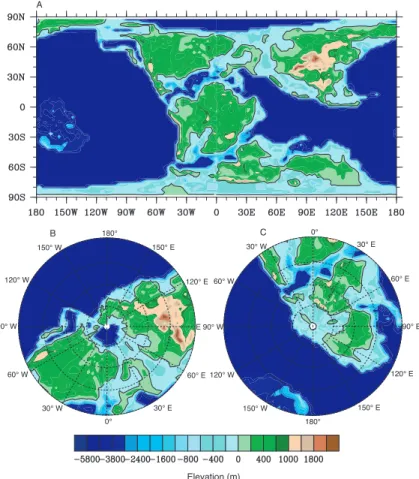
Early Aptian geography, topography, and bathymetry are presented in Fig. 2.

Impor-15

tant features of the Aptian geography, topography, and bathymetry include, the lack of a major land mass at the South Pole, an Arctic Ocean with relatively extensive, though shallow, connections to the global oceans, a small North Atlantic, a minimal, extremely shallow South Atlantic, and a narrow sea strait between southeastern Africa and India. The highest elevations are in Central Asia with other minor highs of note in the proto

20

Andean Arc and the proto Cordillera of North America.

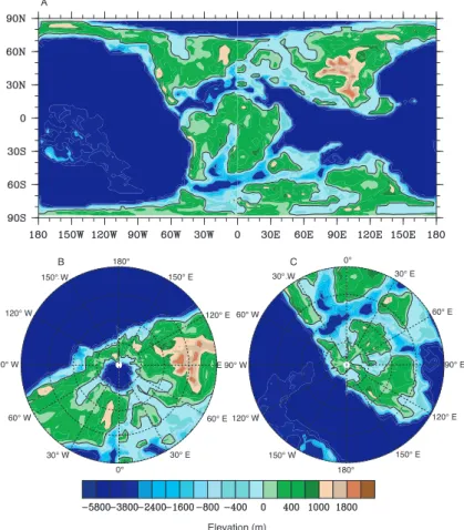
Early Albian geography, topography, and bathymetry are presented in Fig. 3. Impor-tant features of the Albian geography, topography, and bathymetry include a restricted Arctic Ocean, the initiation of Cretaceous interior seaways in North America and east-ern Europe, a deeper Panama Strait, a more open Tethyan region, and a more

exten-25

sive South Atlantic than in the Aptian. The highest elevations are again in Central Asia and there is now a notable high in western Greenland, as well as growth of the North

(11)

CPD

EGU

American Cordillera.

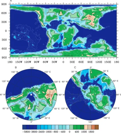
Cenomanian/Turonian boundary geography, topography, and bathymetry are pre-sented in Fig. 4. Important features of the Cenomanian/Turonian boundary geogra-phy, topogrageogra-phy, and bathymetry include a larger and more open North Atlantic with a deeper Panama Strait when compared to the Albian, extensive Cretaceous

inte-5

rior seaways in North America, South America, North Africa, and eastern Europe, an open, though narrow, South Atlantic, and more open flow (compared to the Albian) in the Southern Ocean. The highlands of Central Asia remain the highest elevations on the globe, however, both the proto Andean Arc and the North American Cordillera have grown in elevation and extent and notable highs are beginning to appear on Antarctica.

10

Early Maastrichtian geography, topography, and bathymetry are presented in Fig. 5. Important features of the Maastrichtian geography, topography, and bathymetry include a restricted Arctic Ocean, a larger, deeper North Atlantic with a deep, open Panama Strait, a wider, deeper South Atlantic, a more restricted Tethyan region (relative to the Cenomanian/Turonian boundary), and the decline of interior seaways on all

con-15

tinents. Though still the highest and largest mountainous region, the highlands of Central Asia have decreased in elevation and the North American Cordillera continues to grow. Highlands on Antarctica have expanded and reached elevations in excess of 1000 m.

The global vegetation distributions for all four time slices are presented along with a

20

detailed key in Fig. 6. The land surface types, with the exception of ocean and land ice, represent complete, though general, vegetation biomes. In the early Aptian (Fig. 6a) high latitude and elevation biomes are moist, open canopy, evergreen or mixed forests with a shrub understory. Middle latitude biomes are closed canopy, broad leaved, moist evergreen forest, and tropical biomes range from closed canopy, broad leaved,

25

dry deciduous forest through Savanna to deciduous shrublands.

In the early Albian (Fig. 6b), high latitudes and elevations continue to be character-ized by moist, open canopy, evergreen or mixed forests with a shrub understory. Mid-latitude biomes continue to be dominated by closed canopy, moist, broad leaved

(12)

ever-CPD

EGU

green forests, though some locations are now Savanna (southern South American and Africa; Fig. 6b) or closed canopy, dry, broad leaved, deciduous forest (the rain shadow of the North American Cordillera and the southern Andes; Fig. 6b). Tropical biomes are largely Savanna and dry, deciduous shrublands. Closed canopy, moist, broad leaved, evergreen forests are present in some coastal and island regions (Fig. 6b).

5

At the Cenomanian/Turonian boundary (Fig. 6c), the high latitudes are dominated by evergreen forest, either closed or open canopy, with a shrub understory (Fig. 6c). Mid-latitude vegetation is a mix of closed canopy, evergreen conifer forest at lower elevations and Savanna and evergreen shrubland in higher or dryer locations (Fig. 6c). Tropical latitude biomes range from open canopy, mixed forest with a shrub understory

10

through Savanna to evergreen shrublands (Fig. 6c).

Early Maastrichtian high latitudes are dominated by mixed forest that grades equa-torward into open canopy, evergreen forest with a shrub understory (Fig. 6d). High elevations on Antarctica are occupied by land ice (alpine glaciers and ice fields). Mid-latitude vegetation is a mix of open and closed canopy evergreen forest with some

15

evergreen shrubland or Savanna at higher elevations (Fig. 6d). Tropical vegetation is generally drier with extensive areas of closed canopy, dry, broad leaved deciduous forest, Savanna, and dry shrubland (Fig. 6d); some coastal and island locations are closed canopy, broad leaved, moist evergreen forest.

4 Conclusions

20

The development of surface boundary conditions is a necessary and time-consuming aspect of paleoclimate modeling. In an effort to reduce the community integrated effort devoted to boundary condition development, we present surface boundary conditions for four Cretaceous time slices. These boundary conditions have been modified to integrate well with modern, coupled climate system models and are available upon

25

request. The large-scale features represented in these boundary conditions are robust in both the temporal and spatial regimes and appropriate to the level of detail captured

(13)

CPD

EGU

in modern climate models. It is our hope that these boundary conditions will provide a basis for other researchers interested in Cretaceous climate history and that their use will promote a level of comparability between modeling simulations conducted by multiple research groups and hence facilitate growth in our understanding of warm climate dynamics and function.

5

Acknowledgements. The authors thank S. L. Wing, B. A. LePage, J. H. A. van

Konijnenburg-van Cittert and H. Pfefferkorn for commentary on the global vegetation distributions. This re-search is funded by Senter Novem.

References

Archangelsky, S.: Evidences of an Early Cretaceous floristic change in Patagonia, Argentina,

10

VII International Symposium on Mesozoic Terrestrial Ecosystems. Asociacion Paleontologica Argentina, Buenos Aires, 2001.

Archangelsky, S. (Ed.): La flora cretacica del Grupo Baquero, Santa Cruz, Argentina. Mono-grafias Del Museo Argentino De Ciencias Naturales, 4, Buenos Aires. 2003.

Barron, E. J.: Climatic Implications of the Variable Obliquity Explanation of

Cretaceous-15

Paleogene High-Latitude Floras, Geology, 12, 595–598, 1984.

Bonan, G. B.: The land surface climatology of the NCAR Land Surface Model coupled to the NCAR Community Climate Model, J. Climate, 11, 1307–1326, 1998.

Collins, W. D. Bitz, C. M., Blackmon, M. L., et al.: The Community Climate System Model version 3 (CCSM3), J. Climate, 19, 2122–2143, 2006.

20

Crane, P. R., Friis, E. M., and Pedersen, K. R.: The origin and early diversification of an-giosperms, Nature, 374, 27–33, 2002.

Dam, G., Nohr-Hansen, H., Flemming, G. C., Bojesen-Koefoed, J. A., and Troels, L.: The oldest Marine Cretaceous sediments in west Greenland (Umiivik-1 borehole) – record of the Cenomanian-Turonian anoxic event, Geol. Greenland Surv. Bull, 189, 128–137, 1998.

25

DeConto, R. M. and Pollard, D.: A coupled climate-ice sheet modeling approach to the Early Cenozoic history of the Antarctic ice sheet, Palaeogeography Palaeoclimatology Palaeoe-cology, 198, 39–52, 2003.

(14)

CPD

EGU

Dijkstra, H. A. and Sewall, J. O.: Climate model boundary conditions for four Cretaceous time slices, Eos Trans. AGU, 87(52), Fall Meet. Suppl., Abstract PP23C-1769, 2006.

Exon, N. F., Kennett, J. P., Malone, M. J., et al.: Proc. ODP, Init. Repts., 189: College Station, TX (Ocean Drilling Program), 2001.

Huber, M. and Sloan, L. C.: Heat transport, deep waters, and thermal gradients: Coupled

5

simulation of an Eocene Greenhouse Climate, Geophysi. Res. Lett., 28, 3481–3484, 2001. Jungclaus, J. H., Haak, H., Latif, M., and Mikolajewicz, U.: Arctic-North Atlantic interactions and

multidecadal variability of the meridional overturning circulation, J. Climate, 18, 4013–4031, 2005.

Markwick, P. J. and Valdes, P. J.: Palaeo-digital elevation models for use as boundary

condi-10

tions in coupled ocean-atmo sphere GCM experiments: a Maastrichtian (late Cretaceous) example, Palaeogeography Palaeoclimatology Palaeoecology, 213, 37–63, 2004.

Meschede, M. and Frisch, W.: A plate tectonic model for the Mesozoic and early Cenozoic history of the Caribbean plate, Tectonophysics, 296, 269–291, 1998.

Mohr, B. and Lazarus, D. B.: Paleobiogeographic distribution of Kuylisporites and its

possi-15

ble relationship to the extant fern genus Cnemidaria (Cyatheaceae), Annals of the Missouri Botanical Garden, 81, 1994.

Mohr, B. and Rydin, C.: Trifurcatia Flabellata n. gen. n. sp., a putative monocotyledon an-giosperm from the Lower Cretaceous Crato Formation (Brazil), Geowiss. Reihe, 5, 335–344, 2002.

20

Otto-Bliesner, B. L., Brady, E. C., and Shields, C.: Late Cretaceous ocean: Coupled simulations with the National Center for Atmospheric Research Climate System Model, J. Geophys. Res.-Atmos., 107, doi:10.1029/2001JD000821, 2002.

Otto-Bliesner, B. L. and Upchurch Jr., G. R.: Vegetation-induced warming of high-latitude re-gions during the Late Cretaceous period, Nature, 385, 804–807, 1997.

25

Ross, M. I. and Scotese, C. R.: A hierarchical tectonic model of the Gulf of Mexico and Caribbean region, Tectonophysics, 155, 139–168, 1988.

Saward, S. A. (Ed.): A global view of Cretaceous vegetation patterns. Geological Society of America Special Paper 267, 267. Geological Society of America, Boulder, Colorado. 1992. Scotese, C. R.: Atlas of Earth History, Volume 1, Paleogeography, 1. PALEOMAP Project,

30

Arlington, TX, 52 pp., 2001.

Sewall, J. O. and Sloan, L. C.: Come a little bit closer: A high-resolution climate study of the early Paleogene Laramide foreland, Geology, 34, 81–84, 2006.

(15)

CPD

EGU

Sloan, L. and Barron, E. J.: Paleogene climatic evolution: a climate model investigation of the influence of continental elevation and sea-surface temperature upon continental climate, in: Eocene-Oligocene climatic and biotic evolution, edited by: Prothero, D. R. and Berggren, W. A., Princeton University Press, Princeton, NJ, pp. 202 -217, 1992.

Spicer, R. A., Ahlberg, A., Herman, A. B., Kelley, S. P., Raikevich, M. I., and Rees, P. M.:

5

Palaeoenvironment and ecology of the middle Cretaceous Grebenka flora of northeastern Asia, Palaeogeography Palaeoclimatology Palaeoecology, 184, 65–105, 2002.

Spicer, R. A. and Chapman, J. L.: Climate Change and the Evolution of High-latitude Terrestrial Vegetation and Floras, TREE, 5, 279–284, 1990.

Spicer, R. A. and Herman, A. B.: The Albian-Cenomanian flora of the Kukpowruk River, western

10

North Slope, Alaska: stratigraphy, palaeofloristics, and plant communities, Cretaceous Res., 22, 1–40, 2001.

Vakhrameev, V. A.: Jurassic and Cretaceous floras and climates of the Earth. Cambridge Uni-versity Press, Cambridge. 1991.

van Waveren, I. M., van Konijnenburg-van Cittert, J. H. A., van der Burgh, J., and Dilcher, D.

15

L.: Macrofloral remains from the Lower Cretaceous of the Leiva region (Columbia), Scripta Geologica, 123, 1–39, 2002.

Wajsowicz, R. C.: The response of the Indo-Pacific throughflow to interannual variations in the Pacific wind stress. Part I: Idealized geometry and Variations, J. Phys. Oceanogr., 25, 1805–1826, 1995.

20

Wajsowicz, R. C.: The response of the Indo-Pacific throughflow to interannual variation s in the Pacific wind stress. Part II: Realistic geometry and ECMWF wind stress anomalies for 1985–89, J. Phys. Oceanogr., 26, 2589–2610, 1996.

(16)

CPD

Printer-friendly Version Interactive Discussion EGU -5800 -2800 -800 400 2200 1800 1400 1000 800 200 0 -200 -400 -600 -1200 -1600 -2000 -2400 -3800 -4800 -5800 -2400 -800 -400 0 400 1800 Elevation (m) sea level

Fig. 1.Detailed key of topography and bathymetry. Blue colors indicate ocean while greens and browns represent land. Darker blues are deep water, lighter blues are shallow. Lower elevation land is represented in greens and higher elevations are brown. In general, the contour interval is greater at the extremes of the color bar and smaller near the land/sea boundary.

(17)

CPD

Printer-friendly Version Interactive Discussion EGU A Elevation (m) B C 0° 30° E 60° E 120° E 150° E 180° 150° W 120° W 90° W 60° W 30° W 0° 30° E 60° E 90° E 120° E 150° E 180° 150° W 120° W E 90° W 60° W 30° W

Fig. 2. Early Aptian geography, topography, and bathymetry. The color bar is as explained in Fig. 1 and the land/sea boundary is represented by the single black contour. The three panels give different projections of the same dataset. (A) Cylindrical Equidistant; (B) North Polar Projection (southern limit of 30◦ N); (C) South Polar Projection (northern limit of 30◦ S).

(18)

CPD

Fig. 3. Early Albian geography, topography, and bathymetry. The color bar is as explained in Fig. 1 and the land/sea boundary is represented by the single black contour. The three panels give different projections of the same dataset. (A) Cylindrical Equidistant; (B) North Polar Projection (southern limit of 30◦ N); (C) South Polar Projection (northern limit of 30◦ S).

(19)

CPD

Printer-friendly Version Interactive Discussion EGU B C C A Elevation (m) 0° 30° E 60° E 120° E 150° E 180° 150° W 120° W 90° W 60° W 30° W 0° 30° E 60° E 90° E 120° E 150° E 180° 150° W 120° W E 90° W 60° W 30° W

Fig. 4.Cenomanian/Turonian boundary geography, topography, and bathymetry. The color bar is as explained in Fig. 1 and the land/sea boundary is represented by the single black contour. The three panels give different projections of the same dataset. (A) Cylindrical Equidistant; (B) North Polar Projection (southern limit of 30◦ N); (C) South Polar Projection (northern limit of

(20)

CPD

Fig. 5. Early Maastrichtian geography, topography, and bathymetry. The color bar is as ex-plained in Fig. 1 and the land/sea boundary is represented by the single black contour. The three panels give different projections of the same dataset. (A) Cylindrical Equidistant; (B) North Polar Projection (southern limit of 30◦ N); (C) South Polar Projection (northern limit of 30◦ S).

(21)

CPD

EGU 150W 120W 90W 60W 30W 0 30E 60E 90E 120E 150E 180

90 N 60 N 30 N 0 30 S 60 S 90 S 90 N 60 N 30 N 0 30 S 60 S 90 S

180 150W 120W 90W 60W 30W 0 30E 60E 90E 120E 150E 180 C

A B

D

Ocean Land Ice

High altitude/latitude evergreen conifer closed canopy forest

High altitude/latitude mixed forest with equal percentage broad vs needle leaf and evergreen vs deciduous

Low altitude/latitude evergreen conifer closed canopy forest

Closed canopy, broad leaved, moist evergreen forest

Closed canopy, broad leaved, dry deciduous forest

Savanna: dry, low understory with sparse broad leaved overstory

High altitude/latitude moist, open canopy evergreen forest with shrub understory Low altitude/latitude moist, open canopy, mixed evergreen/deciduous, forest with shrub understory

Wet or cool shrubland (evergreen) Dry or warm shrubland (deciduous)

Fig. 6. Global vegetation distribution for four Cretaceous time slices . (A) early Aptian; (B) early Albian; (C) Cenomanian/Turonian boundary; (D) early Maastrichtian. Vegetation and land surface types are presented as generalized biomes as described in the figure key.