HAL Id: hal-00295634
https://hal.archives-ouvertes.fr/hal-00295634
Submitted on 7 Mar 2005
HAL is a multi-disciplinary open access
archive for the deposit and dissemination of
sci-entific research documents, whether they are
pub-lished or not. The documents may come from
teaching and research institutions in France or
abroad, or from public or private research centers.
L’archive ouverte pluridisciplinaire HAL, est
destinée au dépôt et à la diffusion de documents
scientifiques de niveau recherche, publiés ou non,
émanant des établissements d’enseignement et de
recherche français ou étrangers, des laboratoires
publics ou privés.
mechanisms on polar stratospheric cloud formation at
local and synoptic scales during the 1999-2000 Arctic
winter
S. H. Svendsen, N. Larsen, B. Knudsen, S. D. Eckermann, E. V. Browell
To cite this version:
S. H. Svendsen, N. Larsen, B. Knudsen, S. D. Eckermann, E. V. Browell. Influence of mountain
waves and NAT nucleation mechanisms on polar stratospheric cloud formation at local and synoptic
scales during the 1999-2000 Arctic winter. Atmospheric Chemistry and Physics, European Geosciences
Union, 2005, 5 (3), pp.739-753. �hal-00295634�
www.atmos-chem-phys.org/acp/5/739/ SRef-ID: 1680-7324/acp/2005-5-739 European Geosciences Union
Chemistry
and Physics
Influence of mountain waves and NAT nucleation mechanisms on
polar stratospheric cloud formation at local and synoptic scales
during the 1999–2000 Arctic winter
S. H. Svendsen1, N. Larsen1, B. Knudsen1, S. D. Eckermann2, and E. V. Browell3
1Danish Meteorological Institute, Copenhagen, Denmark 2Naval Research Laboratory, Washington DC, USA 3NASA Langley Research Center, Hampton, Virginia, USA
Received: 30 June 2004 – Published in Atmos. Chem. Phys. Discuss.: 20 August 2004 Revised: 19 October 2004 – Accepted: 28 February 2005 – Published: 7 March 2005
Abstract. A scheme for introducing mountain wave-induced
temperature pertubations in a microphysical PSC model has been developed. A data set of temperature fluctuations at-tributable to mountain waves as computed by the Moun-tain Wave Forecast Model (MWFM-2) has been used for the study. The PSC model has variable microphysics, en-abling different nucleation mechanisms for nitric acid trihy-drate, NAT, to be employed. In particular, the difference between the formation of NAT and ice particles in a sce-nario where NAT formation is not dependent on preexisting ice particles, allowing NAT to form at temperatures above the ice frost point, Tice, and a scenario, where NAT
nucle-ation is dependent on preexisting ice particles, is examined. The performance of the microphysical model in the different microphysical scenarios and a number of temperature sce-narios with and without the influence of mountain waves is tested through comparisons with lidar measurements of PSCs made from the NASA DC-8 on 23 and 25 January during the SOLVE/THESEO 2000 campaign in the 1999–2000 winter and the effect of mountain waves on local PSC production is evaluated in the different microphysical scenarios. Mountain waves are seen to have a pronounced effect on the amount of ice particles formed in the simulations. Quantitative compar-isons of the amount of solids seen in the observations and the amount of solids produced in the simulations show the best correspondence when NAT formation is allowed to take place at temperatures above Tice. Mountain wave-induced
temper-ature fluctuations are introduced in vortex-covering model runs, extending the full 1999–2000 winter season, and the effect of mountain waves on large-scale PSC production is estimated in the different microphysical scenarios. It is seen
Correspondence to: S. H. Svendsen
that regardless of the choice of microphysics ice particles only form as a consequence of mountain waves whereas NAT particles form readily as a consequence of the synoptic con-ditions alone if NAT nucleation above Ticeis included in the
simulations. Regardless of the choice of microphysics, the inclusion of mountain waves increases the amount of NAT particles by as much as 10%. For a given temperature sce-nario the choice of NAT nucleation mechanism may alter the amount of NAT substantially; three-fold increases are easily found when switching from the scenario which requires pre-existing ice particles in order for NAT to form to the scenario where NAT forms independently of ice.
1 Introduction
Polar stratospheric clouds (PSCs) are known to be of vi-tal importance to ozone-depleting processes in the polar re-gions (Tolbert and Toon, 2001). In particular, the formation of solid PSC particles (ice and nitric acid trihydrate (NAT) particles) is important since these particles may grow large enough for gravitational sedimentation to have an impact, thereby depleting the stratosphere of water and nitrogen com-pounds. The removal of these compounds serves to enhance the ozone-depleting conditions (WMO, 1999).
In the northern polar stratosphere synoptic temperatures usually hover around the existence temperature for NAT (WMO, 1999). Consequently, the additional cooling caused by mountain waves may be of importance to the produc-tion of solid PSC types in the northern polar vortex. Moun-tain waves are known to cause the formation of solid PSC types (Carslaw et al., 1998a,b) and the locally produced solid PSCs may exist at vast distances downstream (Carslaw et al.,
1999). The presence of NAT particles in the Arctic strato-sphere does not appear to be sporadic; in a multi-year study of lidar data from Ny ˚Alesund, Biele et al. (2001) found wide-spread presence of NAT particles interspersed with liq-uid aerosol. In order to be able to produce reasonable es-timates of the load of solid type PSCs in the Arctic, it is therefore important to be able to evaluate the amount of PSCs produced in mountain waves compared to the amount of syn-optically produced PSCs. Lidar observations are an excellent tool for studying local-scale PSC phenomena in great detail (Toon et al., 2000). Detailed studies of lidar observations of mountain wave PSCs combined with microphysical and op-tical modelling have been carried out by e.g. Hu et al. (2002) and Fueglistaler et al. (2003).
According to a study of mountain wave PSCs by Fueglistaler et al. (2003), ECMWF trajectories lack the abil-ity to reproduce the cooling rates observed in mountain waves. In the present study, a method for incorporating mountain wave effects in microphysical PSC simulations on local as well as synoptic scales has been developed, thereby allowing for an estimate of the importance of mountain wave effects on the PSC load.
Whereas the existence of NAT particles in polar strato-spheric clouds is well established (Voigt et al., 2000), the formation mechanism of NAT is still debated. NAT is be-lieved to form by heterogeneous nucleation on pre-existing ice particles, requiring temperatures below Ticeat some point
(Carslaw et al., 1998a,b), but recent studies have indicated the need for NAT nucleation mechanisms which are indepen-dent of the existence of ice particles, only requiring temper-atures below the existence temperature for NAT, a condition which is easier to meet than the demand for pre-existing ice particles (Drdla et al., 2002; Pagan et al., 2004; Irie et al., 2004). Here, the effect of a proposed nucleation mechanism for NAT which is active above Ticeis examined on both local
and synoptic scales.
In Sect. 2 the microphysical model used for this study is presented and the method for including mountain wave ef-fects in the simulations is introduced in Sect. 2.1. Next, com-parisons between lidar measurements of PSCs and model runs with variable microphysics and with and without moun-tain waves are presented in Sect. 3. Finally, in Sect. 4 the influence of mountain waves and the choice of microphysics on the production of solid PSCs inside the vortex is evaluated for the winter 1999–2000.
2 The microphysical model
Simulations of the PSC production have been made using the Danish Meteorological Institute microphysical PSC model (Larsen, 1991, 2000). The core of the PSC model is a box model which for a given time step calculates the changes in size distributions, chemical composition, and physical phase of an ensemble of particle types. The input to the box model
at each time step is the temperature, pressure, partial pres-sures of H2O and HNO3, the current number densities, and
the amount of bound acid and water in each size bin of the different aerosol types, and the box model returns new val-ues of these parameters in each size bin. Mixtures of four different particle types are recognised by the model: 1) Liq-uid particles assumed to be sulphate aerosols turning into su-percooled ternary H2O-H2SO4-HNO3solutions (STS) at low
temperatures through uptake of HNO3and H2O, 2) frozen
sulphate aerosols assumed to be sulphuric acid tetrahydrate, SAT, 3) NAT particles with inclusions of SAT, and 4) ice par-ticles with inclusions of NAT and SAT. Each of the four dif-ferent particle types has its own size distribution. The size distributions are discretized into N size bins on a geometric volume scale. Within a given size distribution particles are shifted to higher or lower radius bins through vapour depo-sition and evaporation. When phase trandepo-sitions occur (e.g. all NAT evaporating to form a SAT particle) particles are transferred from one size distribution to another. During this transfer the particles are assumed to have an unaltered radius. When calculating the evaporation and condensational growth of liquid, NAT, and ice particles, vapour pressures over STS are taken from Luo et al. (1995), vapour pressures over NAT are taken from Hanson and Mauersberger (1988), and vapour pressures over ice are taken from Marti and Mauersberger (1993). Ice particles form by homogeneous nucleation out of STS solutions at temperatures 3–4 K below the ice frost point, Tice, and a homogeneous nucleation rate, derived from
experimental data, is used in the simulations (Koop et al., 2000).
Recently, studies have been published indicating the need for a freezing process active above Tice in order to explain
observations of solid PSC particles (Drdla et al., 2002; Pa-gan et al., 2004; Irie et al., 2004; Larsen et al., 2004). As an example of a NAT nucleation mechanism capable of gen-erating NAT at temperatures above the ice frost point, NAT nucleation in the present study is described by the nucleation rate of nitric acid dihydrate, NAD, found in Tabazadeh et al. (2002) (assuming an instantaneous conversion of NAD par-ticles to NAT), although corrected by a factor of 0.1 in order to comply with restrictions posed by observations of particle size distributions and gas phase mixing ratios of HNO3
ac-cording to the findings in Larsen et al. (2004). The proposed nucleation mechanism is currently debated, see e.g. Knopf et al. (2002), but it is, to our knowledge, the latest published parameterisation of NAT nucleating out of STS at tempera-tures above Tice and may as such be seen as a useful
repre-sentative of scenarios allowing for NAT nucleation at temper-atures above Tice. Whether this particular nucleation
mecha-nism alone is responsible for any NAT formation at temper-atures above Tice or whether other nucleation mechanisms,
e.g. heterogeneous nucleation (Drdla et al., 2002), are active cannot be concluded from the present study, which only ad-dresses the effect of a single proposed nucleation mechanism for NAT which is active above Ticeas compared to a scenario
where NAT formation requires the presence of ice particles. Note that the choice of nucleation mechanism for NAT will affect the formation of ice particles. If NAT can form at tem-peratures above the ice frost point, ice may nucleate hetero-geneously on preexisting NAT particles as soon as temper-atures drop slightly below Tice instead of only forming by
homogeneous nucleation at temperatures 3–4 K below Tice.
The model is initialised by profiles of HNO3 and H2O
and a background population of sulphuric aerosols. The size distribution of the sulphuric aerosols is based on a SAGE I and SAGE II (Stratospheric Aerosol and Gas Experiment) surface area climatology (Hitchman et al., 1994). Aerosol extinctions are retrieved from the SAGE/SAM stratospheric aerosol climatology Hitchman et al. (1994) by interpolation in latitude and altitude in the tabulation of decadal mean val-ues and converted to surface area densities by the provided formula (Hitchman et al., 1994). Assuming the aerosol is characterised by a lognormal size distribution with median radius 0.0725 µm and geometric standard deviation 1.86, Pinnick et al. (1976), the surface area density is converted to aerosol number density, resulting in values in the order of 10 particles per cm3, consistent with measurements (Schreiner et al., 2003). The HNO3 content is initialised by a LIMS
profile (Gille and Russell, 1984) and the H2Ocontent is
de-scribed as a function of the potential temperature, 2, based on a series of frost point hygrometer measurements in the northern polar vortex (Ovarlez et al., 2004). Comparing the LIMS profile to observations of the HNO3profile made
dur-ing SOLVE/THESEO-2000, Coffey et al. (2002), the LIMS profile is lower than the observations from December and higher than the observations from March. It is our opinion that a profile placed in between the two winter extremes of December and March is a reasonable value to use for the ini-tialisation of the model.
The input to the model is provided by temperature trajec-tories based on ECMWF analyses. The calculation of the trajectories uses 6 hourly ECMWF analyses on a 1.5◦×1.5◦ longitude-latitude grid. The trajectories themselves are cal-culated on an equal-area grid with a grid distance of 139 km and start inside or at the edge of the polar vortex at 9 standard isentropic levels (360 K, 380 K, 400 K, 435 K, 475 K, 515 K, 550 K, 600 K, and 650 K) in the case of the hemispheric sim-ulations and on 11 levels (400 K, 425 K, 450 K, 475 K, 500 K, 530 K, 560 K, 590 K, 600 K, 625 K, and 700 K) in the case of the small-scale simulations. Diabatic cooling is taken into account in the calculations (Morcrette, 1991; Knudsen and Grooss, 2000; Larsen et al., 2002). At each point of a trajec-tory the temperature, pressure, potential temperature, poten-tial vorticity, latitude, and longitude are given. Depending on the number of trajectories and their duration, microphysical simulations on a variety of scales may be performed; from very detailed model runs closely matching the time and lo-cation of different sets of measurements to vortex-covering simulations extending over entire winter seasons.
2.1 Including mountain wave effects in the simulations Temperature fluctuations due to mountain waves may in-fluence the formation of solid type PSCs (Carslaw et al., 1998a). Climatological studies of the stratosphere over Scan-dinavia have shown that practically all ice particle events in this area are attributable to the presence of mountain waves (D¨ornbrack and Leutbecher, 2001). In order to ob-tain reliable estimates of the PSC load, the inclusion of mountain wave effects in the modelling of PSCs is cru-cial. ECMWF reanalyses lack sufficient resolution to resolve the full spectrum of mesoscale mountain waves that occur in the stratosphere, see e.g. (Fueglistaler et al., 2003). To provide estimates of mountain wave influences on the PSC load, mesoscale temperature variances from hindcast runs using Version 2 of the Naval Research Laboratory Moun-tain Wave Forecast Model (MWFM-2) through global anal-ysis fields issued by NASA’s Global Modeling and Analy-sis Office (GMAO) during the Arctic winter of 1999–2000 are used to supplement the ECMWF temperature trajecto-ries. Details of the MWFM-2 algorithms are given by Eck-ermann and Preusse (1999), Hertzog et al. (2002) and Jiang et al. (2004). These fields are issued as averaged gridded wave-induced temperature variance fields on pressure sur-faces, derived from the raw mountain wave ray data gen-erated by the hindcasts, to make them more amenable for use in offline transport simulations. The formation and use of this 1999–2000 gridded product is described in detail by Pierce et al. (2003) and Pagan et al. (2004). An important point to note is that the procedure of avaraging into a grid-ded variance product tends to significantly suppress typical intra-gridbox variability found within unaveraged mountain wave fields (Hertzog et al., 2002; Brogniez et al., 2003) and thus the data product used in this study should be viewed as a working lower bound on likely mesoscale temperature variability due to mountain waves. Thus, any microphysical changes caused by insertion of these mountain wave fields are likely significant.
In this study, the MWFM-2 fields are used to introduce mountain wave-induced temperature fluctuations into the simulations. The MWFM-2 hindcasts and averaging produce daily fields of mountain wave-induced temperature fluctua-tions on a 1◦×1◦grid, specifying the amplitude of the tem-perature fluctuation at seven standard pressure levels (10, 20, 30, 40, 50, 70, and 100 hPa). Through interpolations in pres-sure and time the value of the temperature amplitude is found at the nearest grid point of each trajectory position, thereby producing a data base of mountain wave-induced tempera-ture fluctuations at the times and locations of the trajectories. When running the microphysical simulations, different tem-perature scenarios with and without the inclusion of moun-tain wave effects can be examined: Case 1: T =T0, Case
2: T =T0−TA, Case 3: T =T0−TA−Tcorr, where T is the
temperature used as input in the microphysical simulations,
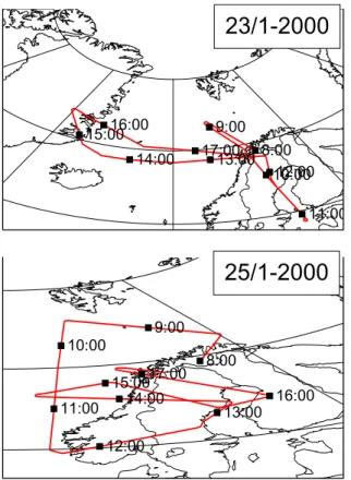
8:00 9:00 10:00 11:00 12:00 13:00 14:00 15:00 16:00 17:00 8:00 9:00 10:00 11:00 12:00 13:00 14:00 15:0016:00 17:00
25/1-2000
23/1-2000
Fig. 1. Flight tracks of the DC-8 flights of 23 and 25 January 2000,
respectively.
Table 1. Threshold values for type classification of DC-8 lidar
mea-surements. B: Backscatter ratio, D: Depolarisation.
DC-8 lidar threshold values
B D(%)
PSC 1b 0.18≤B D<2.5 PSC 1a 0.18≤B≤5.0 D≥2.5 PSC 2 B>5.0 D≥2.5
analysis, TAis the mountain wave-induced temperature
am-plitude, and Tcorr is an additional temperature correction,
based on temperature restrictions posed by the presence of ice particles in observations. This additional correction will be described in further detail below. Subtraction of the am-plitude of the mountain wave perturbation in cases 2 and 3 corresponds to the maximal lowering of the temperatures and one should therefore interpret these results as lower limits of the temperature.
3 Comparing model runs and lidar measurements
Given the high altitude and time resolution of lidar measure-ments, very detailed information about the observed aerosols can be provided by such measurements. In order to make comparisons between observations and model results, it is important to ensure that the model results closely match the time and location of the measurements. In the present study, lidar data from the NASA DC-8 flights of 23 and 25 Jan-uary 2000, during the SOLVE/THESEO 2000 campaign have been considered. Data from these flights have been studied extensively by Hu et al. (2002) and Fueglistaler et al. (2003). A summary of the SOLVE/THESEO 2000 campaign can be found in Newman et al. (2002). A description of the lidar system used for the measurements can be found in Browell (1989) and Browell et al. (1990). A map showing the flight tracks of the two flights is shown in Fig. 1. Sets of back tra-jectories have been initiated along the flight tracks. Running these trajectories produces information about the aerosol at the position and time of the lidar measurements according to the microphysical model.
The accuracy of the temperatures and the mountain wave corrections can be evaluated by considering the restrictions on the temperatures posed by the presence of ice particles. In areas where ice is observed, the temperature must nec-essarily be equal to or colder than the ice frost point, Tice.
By keeping track of the times and altitudes where ice parti-cles are observed one may compare the model temperatures in these areas to Tice. In the DC-8 data, aerosol backscatter
ratios at 603 nm greater than 5.0 with enhanced depolarisa-tion (>2.5%) are considered to be ice particles, see Table 1. Comparisons of the model temperatures and Tice indicate a
warm-bias in the model temperatures and an additional tem-perature correction, Tcorr, is thus introduced. Tcorris defined
as the average difference between the model temperature and
Tice in those areas where ice particles are observed. It is
as-sumed that the additional temperature correction is associ-ated with an under-estimation of the mountain wave-induced temperature fluctuations and Tcorr is only introduced in the
simulations if the mountain wave-induced temperature am-plitude TA exceeds a value of 0.5 K. The value of Tcorr is
found to be 1.16 K for 23 January 2000, and 3.70 K for 25 January 2000.
The model allows the calculation of the backscatter ratio and depolarisation based on a T-matrix calculation code as described in Larsen et al. (2004). A number of assumptions about the shape of the particles and their refractive indices must be made and the calculated backscatter ratio and depo-larisation will be rather sensitive to the choice of these pa-rameters. Hence, the calculated optical variables are only suited for general qualitative comparisons with the measured data and not for detailed, quantitative comparisons. The dif-ference in temporal and altitudinal resolution between the measured and modelled quantities as well as the limited res-olution (1◦×1◦) of the mountain wave-induced temperature
8 10 12 14 16 18 14 16 18 20 22 24 26 8 10 12 14 16 18 14 16 18 20 22 24 26 8 10 12 14 16 18 14 16 18 20 22 24 26 8 10 12 14 16 18 14 16 18 20 22 24 26 A
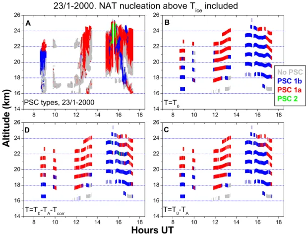
23/1-2000. NAT nucleation above T
iceincluded
PSC types, 23/1-2000 B No PSC PSC 1b PSC 1a PSC 2 T=T0 C T=T 0-TA D T=T 0-TA-Tcorr
A
ltitu
d
e
(k
m
)
Hours UT
Fig. 2. Observed and modelled PSC types for 23 January, 2000. Grey areas in the plots of measured data represent valid data with backscatter
values less than the minimum threshold value for PSC presence whereas white areas indicate lack of valid data. Panel (A) shows the observed PSC types, panel (B) shows the PSC types according to the microphysical model in the T =T0scenario, panel (C) shows the modelled PSC
types in the T =T0−TAscenario, and panel (D) shows the modelled PSC types in the T =T0−TA−Tcorrscenario.
corrections point to overall qualitative comparisons instead of detailed point-by-point comparisons. Therefore, com-parisons between observational data and modelled data are based on cloud types instead of a direct comparison of the optical variables. In the case of the observations, type dis-tinction is made by considering the backscatter ratio and the depolarisation. Such a cloud type distinction is only possible when both the backscatter ratio and the depolarisation are available and, hence, the type plots presented here only rep-resent the areas where both types of data are prep-resent. Points where the backscatter ratio B lies in the interval 0.18≤B≤5.0 and the depolarisation D is larger than 2.5% are classified as type 1a PSCs whereas points where 5.0<B and 2.5%<D are classified as type 2 PSCs and points where the depolarisa-tion is smaller than 2.5% and the backscatter ratio is higher than 0.18 (0.18<B and D<2.5%) are considered to be type 1b PSCs. An overview of the PSC type classification scheme for the observational data is given in Table 1. It should be noted that in the present paper only the aerosol backscatter ratio and not the total backscatter ratio is considered.
Observations of PSCs indicate that very often there are both liquid and solid particles present in the cloud (Biele et al., 2001; Larsen et al., 2004). Whether a given PSC obser-vation will be classified as a type 1a or type 1b PSC depends on whether NAT particles or STS particles dominate the opti-cal signal. When determining the cloud type of a given mod-elled particle distribution it is therefore necessary to have an estimate of the proportions in the mixture of liquid and solid particles which gives rise to a classification as a type 1a or type 1b PSC. In simulations of the volume density of STS and NAT particles and the total colour index and extinction a clear switch in the colour index and extinction from what would be considered a type 1b cloud to a type 1a cloud took place when the surface area density of NAT was approxi-mately 5% of the surface area density of STS, see Fig. 5 in (Larsen et al., 2004). When classifying the PSC type of a given model data point this is used as a threshold value to separate PSC 1a from PSC 1b; if the surface area density of either NAT or ice in a given point constitutes 5% or more of the surface area density of STS particles, the point is classi-fied as a type 1a or type 2 point, respectively. If not, the point is classified as a type 1b point.
8 10 12 14 16 18 14 16 18 20 22 24 26 8 10 12 14 16 18 14 16 18 20 22 24 26 8 10 12 14 16 18 14 16 18 20 22 24 26 8 10 12 14 16 18 14 16 18 20 22 24 26 A
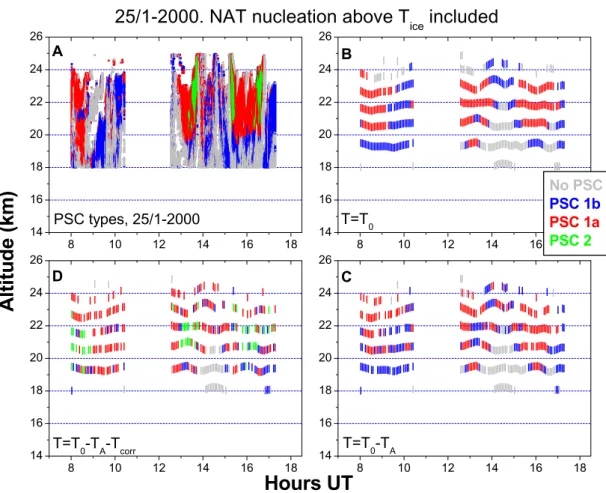
25/1-2000. NAT nucleation above T
ice
included
PSC types, 25/1-2000 B No PSC PSC 1b PSC 1a PSC 2 T=T0 C T=T0-TA D T=T 0-TA-TcorrA
ltitu
d
e
(k
m
)
Hours UT
Fig. 3. Observed and modelled PSC types for 25 January 2000. Grey areas in the plots of measured data represent valid data with backscatter
values less than the minimum threshold value for PSC presence whereas white areas indicate lack of valid data. Panel (A) shows the observed PSC types, panel (B) shows the PSC types according to the microphysical model in the T =T0scenario, panel (C) shows the modelled PSC
types in the T =T0−TAscenario, and panel (D) shows the modelled PSC types in the T =T0−TA−Tcorrscenario.
Comparisons of the PSC type distribution in the measured and the modelled data are shown in Fig. 2 for 23 January 2000, and Fig. 3 for 25 January 2000. NAT nucleation above
Ticehas been included in the simulations. In the figures, the
upper left panel (A) shows the PSC type distribution in the measurement data. The upper right panel (B) shows model results from the T =T0 scenario, the lower right panel (C)
shows the results from the T =T0−TA scenario and the
re-sults from the T =T0−TA−Tcorr scenario are shown in the
lower left panel (D). In the simulations of the two DC-8 flights NAT nucleation above Ticehas been included.
In the case of 23 January 2000 (see Fig. 2), areas of all three PSC types are seen in the observations. When con-sidering the model data it is seen that in the case where no temperature corrections have been introduced (panel B) the model handles the presence of PSC 1a and PSC 1b reason-ably well. Around 09:00 UT the observations indicate PSC 1a around 21–23 km followed by PSC 1b from 19 to 21 km. In the model, this region shows both PSC 1a and PSC 1b as well, although the PSC 1a field extends too far downwards and the PSC 1b field is lying too low. Around 10:00 UT
the observations indicate an area of no PSCs between 15 and 19 km and from 22 to 23 km, possibly with small amounts of PSC 1a clouds in the lower area. No valid data is present covering the intermediate altitude interval. In the model, the entire altitude interval contains PSCs, with a small area of PSC 1a at the top of the profile and PSC 1b in the interme-diate and lower part. The next section in the observational data stretches from 12:00 to 13:30 UT in the altitude inter-val from 16 to 24 km and shows no PSCs in the early and/or lower parts of the segment and PSC 1a in the higher part. In the model data PSC 1a is the prominent feature, although the PSCs are seen to extend too low and span a longer time inter-val than the observations. The last segment of the observa-tions show distinct areas of PSC 2 (from 22 to 24 km between 15:30 and 16:00 UT), PSC 1a (from 15:00 to 17:00 UT and from 19 km and upwards) and PSC 1b which is mainly seen from 16:00 to 17:00 UT between 17 and 23 km. In the model data, the PSC 2 field is not reproduced. Ample amounts of PSC 1b are observed as well as PSC 1a, although the PSC 1a field is generally too small. Overall, the model data ap-pears to extend the PSC fields too far downwards, which may
7 8 9 10 11 12 13 14 15 16 17 18 14 16 18 20 22 24 26 7 8 9 10 11 12 13 14 15 16 17 18 14 16 18 20 22 24 26 7 8 9 10 11 12 13 14 15 16 17 18 14 16 18 20 22 24 26
B
NAT nucleation above Tice included
Altitude (km)
Hours UT
C
23/1-2000. T=T
0
-T
A-T
corrNAT nucleation above Tice not included
A
PSC types, 23/1-2000.
Fig. 4. Comparison of measured and modelled PSC types for 23
January 2000. Panel (A) shows the observed PSC types whereas panel (B) shows the modelled PSC types in the microphysical sce-nario where NAT nucleation above the ice frost point is included and panel (C) shows the modelled PSC types in the microphysical scenario where NAT nucleation above the ice frost point is not in-cluded. In both of the model simulations the coldest temperature scenario T =T0−TA−Tcorrhas been used.
be indicative of an altitude bias in the model data. It should be mentioned, however, that the altitude is determined from the pressure of the input trajectories and the scale height, and should be viewed as an approximation. Most notably is the lack of ice particles in the model data considering the rather prominent ice feature seen in the observations. When moun-tain wave effects are included in the simulations (panels C and D) an increase in PSC 1a is seen at the expense of PSC 1b. Ice clouds are only seen in the coldest of the three temper-ature scenarios, (panel D). The PSC 1a field observed around 15:00 UT is not reproduced by the model in any of the three temperature scenarios.
Considering the DC-8 flight of 25 January 2000, all three PSC types are observed as well (see Fig. 3, panel A). The first section of the observational data (from 08:00 to 10:00 UT) shows only PSC 1a and PSC 1b, with PSC 1a dominating the early part of this section and PSC 1b dominating the late part. In the case of the model data the synoptic scenario (panel B) shows a mixture of PSC 1a and PSC 1b as well, although the PSC 1a field extends a little later than what is seen in the observations. The next section of the observational data from 12:30 to 17:00 UT shows three prominent PSC 2 areas
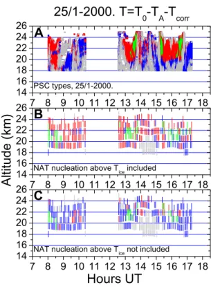
7 8 9 10 11 12 13 14 15 16 17 18 14 16 18 20 22 24 26 7 8 9 10 11 12 13 14 15 16 17 18 14 16 18 20 22 24 26 7 8 9 10 11 12 13 14 15 16 17 18 14 16 18 20 22 24 26
B
NAT nucleation above Tice included
Altitude (km)
C
25/1-2000. T=T
0
-T
A-T
corrNAT nucleation above Tice not included
Hours UT
A
PSC types, 25/1-2000.
Fig. 5. Comparison of measured and modelled PSC types for 25
January 2000. Panel (A) shows the observed PSC types whereas panel (B) shows the modelled PSC types in the microphysical sce-nario where NAT nucleation above the ice frost point is included and panel (C) shows the modelled PSC types in the microphysical scenario where NAT nucleation above the ice frost point is not in-cluded. In both of the model simulations the coldest temperature scenario T =T0−TA−Tcorrhas been used.
surrounded by PSC 1a. The middle part of this section (from 14:00 to 15:30 UT) is a complex mixture of PSC 1a and PSC 1b. In the synoptic model data (panel B) the PSC 1a fields are reproduced reasonably well. Most notable is the complete lack of PSC 2 fields in the synoptic model data. Proceeding to scenarios where mountain wave effects are included (panel C and D) an increase in the amount of PSC 1a is seen at the expense of PSC 1b. Going to the coldest of the three temperature scenarios, T =T0−TA−Tcorr (panel D) areas of
PSC 2 are seen in the model data as well. However, the PSC 2 areas in the latest segment span time intervals which are slightly long compared to the observations and in the first segment (around 08:00 UT) a PSC 2 field is seen in the model data which is not seen in the observations. Given that the amount of PSC 2 in the T =T0−TA−Tcorrseems to be rather
large compared to the observed amount of PSC 2, one may suspect that the value of Tcorrhas been too high in this case.
Tcorr is an average value based on the difference between
Tice and T in the areas where PSC 2 observations are made
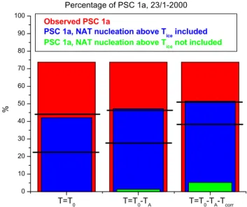
0 10 20 30 40 50 60 70 80 90 100 Percentage of PSC 1a, 23/1-2000 T=T0-TA-Tcorr T=T0-TA T=T0 % Observed PSC 1a
PSC 1a, NAT nucleation above Tice included
PSC 1a, NAT nucleation above Tice not included
Fig. 6. Percentage of PSC 1a in observational and model data for
23 January 2000, for three different temperature scenarios. Model results are shown for two different microphysical scenarios, one where NAT nucleation above Tice is allowed, and one where this is not the case. Horizontal black lines mark the PSC 1a percent-age in simulations where the HNO3content has been changed by
±1 ppbv. The variation in the case where NAT nucleation above Ticeis not included is not discernable on this scale.
0 1 2 3 4 5 Percentage of PSC 2, 23/1-2000 T=T0-TA-Tcorr T=T0-TA T=T0 % Observed PSC 2
PSC 2, NAT nucleation above Tice included
PSC 2, NAT nucleation above Tice not included
Fig. 7. Percentage of PSC 2 in observational and model data for
23 January 2000, for three different temperature scenarios. Model results are shown for two different microphysical scenarios, one where NAT nucleation above Tice is allowed, and one where this is not the case. The variation in the percentage of PSC 2 when vary-ing the HNO3content by ±1 ppbv is not discernable on this scale.
Overall, it seems that the microphysical model is capable of producing PSC type distributions which correspond rea-sonably well with observations. In both the examined cases
the synoptic temperature scenario (T =T0) was unable to
re-solve the observed type 2 PSCs. Going to mountain wave-influenced scenarios resulted in PSC 2 presence at the correct locations, even though indications of an overestimated value of Tcorrwas seen in the case of 25 January 2000. As a whole,
the best agreement between the observations and the corre-sponding simulations is seen in the cases where the influence of mountain waves has been included since these cases seem to result in a better reproduction of the solid PSC types.
The simulations used for comparison with the observa-tion data above all included NAT nucleaobserva-tion at temperatures above Tice. In order to illustrate the difference between the
outcome of simulations with and without this particular nu-cleation mechanism comparisons between the two different microphysical scenarios are shown in Fig. 4 for 23 January 2000, and in Fig. 5 for 25 January 2000. In both of these fig-ures, panel (A) shows the observed distribution of PSC types whereas panel (B) shows the modelled PSC distribution when NAT nucleation above Tice is included in the
simula-tions and panel C shows the modelled PSC distribution when this particular nucleation mechanism is not included in the simulations and NAT forms on pre-existing ice particles in-stead. The coldest temperature scenario, T =T0−TA−Tcorr,
is used in all the simulations.
In the case of 23 January 2000 (Fig. 4), large differences are seen between the two different microphysical scenarios; when NAT nucleation above Tice is allowed (panel B) large
sections of PSC 1a are seen, largely corresponding to the PSC 1a fields seen in the observations (panel A). A stretch of PSC 2 is seen as well, although slightly delayed compared to the observations. Going to the scenario where NAT is only allowed to nucleate on pexisting ice particles the model re-sults are completely dominated by PSC 1b and only sporadic traces of PSC 1a are seen. This is not in correspondence with the observations which show ample amounts of PSC 1a.
The comparison for 25 January 2000, is shown in Fig. 5. The simulation where NAT only forms by nucleation on pre-existing ice particles (panel C) is dominated by PSC 1b (panel C), but shows PSC 2 fields in the correct positions. Compared to the measurements (panel A) the amount of PSC 1a is underestimated in this scenario. In the case where NAT nucleation above Tice is allowed (panel B) much more
pro-nounced fields of PSC 1a are seen, which corresponds better with the observations than the case where NAT nucleation above Ticeis not allowed (panel C). Both microphysical
sce-narios display a PSC 2 area around 08:00 UT which is not seen in the observations, an indication that the final tempera-ture correction Tcorrmay be over-estimated in the case of 25
January 2000.
In the qualitative comparisons between observations and simulations described above indications of a preference for mountain wave-perturbed scenarios where NAT nucleation above Ticeis allowed was found. In the following, this
qual-itative analysis is extended to a quantqual-itative one based on the overall PSC statistics of the entire DC-8 flights and the
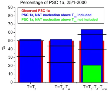
corresponding model simulations. For the sections of the model data which correspond to areas where both backscat-ter ratio and depolarisation data are available and, hence, a PSC type classification is possible, it is investigated whether or not any solid PSCs are present in the model data and the percentage of model points containing either PSC 1a or PSC 2 can be determined. The percentage of PSC 2 and PSC 1a in the observational data (red columns) and in the simula-tions is shown in Fig. 6 and Fig. 7 for 23 January 2000, and in Fig. 8 and Fig. 9 for 25 January 2000. In the figures, the percentages of PSC 1a and PSC 2 in the model data are deter-mined for two sets of model data: one where NAT nucleation above Tice is allowed as described earlier in this paper (blue
columns), and one where NAT nucleation above Tice is not
allowed (green columns). In the latter case, NAT forms on preexisting ice particles.
For both 23 and 25 January 2000, the percentage of PSC 1a in the model data shows the best correspondence with the measurements when NAT nucleation above Ticeis included
(see Fig. 6 and Fig. 8) than when this is not the case. When NAT nucleation above Tice is included in the microphysics
the percentage of PSC 1a in the model data is of the same order of magnitude as the percentage of PSC 1a in the obser-vations whereas the percentage of PSC 1a in the case where NAT nucleation is not included is much smaller. In the case of the PSC 1a, the influence of mountain waves is crucial in the case where NAT nucleation above Ticeis not included in
the microphysics: In this case PSC 1a is only seen as a conse-quence of mountain waves whereas PSC 1a is seen in ample amounts already as a consequence of the synoptic conditions alone when NAT nucleation above Tice is allowed. For both
the days considered here, the synoptic temperatures alone were sufficient to generate the majority of the observed PSC 1a and in such cold cases where the synoptic temperatures al-ready are below TN AT any additional mountain wave cooling
will not cause any large changes. In other cases, where the synoptic temperatures are warmer, mountain wave cooling may have a larger influence on the amount of NAT particles in the scenario where NAT nucleation is allowed above Tice.
In a recent study it was established that PSC 1a obser-vations from the early part of the winter 1999–2000 could not be explained by the presence of mountain waves and that some NAT nucleation mechanism active above the ice frost point was necessary in order to explain the observations (Pa-gan et al., 2004). The present work supports this conclusion since, even in the presence of mountain waves, the amount of PSC 1a produced when there is no NAT nucleation above
Tice does not correspond to the amount of PSC 1a seen in
observations. When NAT nucleation above Tice is active a
better correspondence between observational data and model data is seen.
In the case of the PSC 2, the influence of mountain waves is much larger, see Fig. 7 and Fig. 9. In this case, no PSC 2 is seen in the model data when the synoptic temperatures alone are taken into consideration, regardless of the choice
0 10 20 30 40 50 60 70 80 90 Percentage of PSC 1a, 25/1-2000 T=T 0-TA-Tcorr T=T 0-TA T=T 0 % Observed PSC 1a
PSC 1a, NAT nucleation above Tice included
PSC 1a, NAT nucleation above Tice not included
Fig. 8. Same as Fig. 6, but for 25 January 2000.
0 5 10 15 20 25 Percentage of PSC 2, 25/1-2000 T=T 0-TA-Tcorr T=T 0-TA T=T 0 % Observed PSC 2
PSC 2, NAT nucleation above Tice included PSC 2, NAT nucleation above Tice not included
Fig. 9. Same as Fig. 7, but for 25 January 2000. Horizontal black
lines mark the PSC 2 percentage when the HNO3content is varied
by ±1 ppbv. The variation in the case where N AT nucleation above Ticeis not included is not discernable on this scale.
of microphysics. This is in agreement with the findings of D¨ornbrack and Leutbecher (2001), where a climatological study indicated an almost complete dependence on mountain waves for the PSC 2 production over Scandinavia. When mountain wave effects are included PSC 2 is seen in the model data in the coldest scenario (T =T0−TA−Tcorr), on
23 January 2000, but only when NAT nucleation above Tice
is allowed. On 25 January 2000, PSC 2 is observed in both microphysical scenarios in the coldest temperature scenario, although the percentage of PSC 2 is too large, with the largest discrepancy in the case where NAT nucleation above Ticeis
allowed. The fact that the model overestimates the percent-age of PSC 2 on 25 January 2000, may be an indication that the value of Tcorris too large in this case, as mentioned
ear-lier. The influence of the choice of NAT nucleation mech-anism on the percentage of PSC 2 is not surprising; when NAT particles are present, ice may nucleate heterogeneously as soon as small supersaturations with respect to ice occur, whereas much larger supersaturations are needed in order for homogeneous nucleation of ice particles to take place. Over-all, the correspondence between the percentage of PSC 2 in the model data and in the observations seems to be best when NAT nucleation above Ticeis taken into consideration, as was
the case for the PSC 1a. However, in the case of the PSC 2, the impact of mountain waves is much larger compared to the PSC 1a. Type 2 clouds seem to form exclusively as a conse-quence of mountain wave effects, regardless of the choice of microphysics, whereas type 1a clouds are observed already as a consequence of the synoptic conditions.
The sensitivity of the model results towards changes in the amount of HNO3 has been examined by performing
model runs where the initial LIMS profile has been shifted by ±1 ppbv HNO3. The results from these sensitivity runs
are marked in Figs. 6–9 by horizontal black lines (not all cases are marked; in some cases the variation is not discern-able on the scale used in the figures). The amount of model data points classified as PSC 1a varies between the different HNO3 scenarios, but the differences between the different
microphysical scenarios and temperature scenarios are sta-ble under the variations in the HNO3profile. It is seen from
Figs. 6–9 that the solid PSC percentage can decrease if the amount of HNO3is increased. This has to do with the way
solid PSCs are defined in the type discrimination algorithm, where a data point is defined as a PSC 1a or PSC 2 point if the surface area density of either NAT or ice constitutes 5% or more of the surface area density of STS. Changing the mix-ing ratio of HNO3will affect both the surface area density of
STS and the solid particle types. In particular, raising TN AT
by increasing the mixing ratio of HNO3may cause changes
in the surface area density of NAT because the cooling rate at the point where the temperature drops below TN AT greatly
affects the size distribution of the nucleating NAT particles, e.g. forming a few large NAT particles instead of a lot of small particles.
4 The influence of mountain waves on large-scale PSC production
In Sect. 3 it was shown that mountain waves may have a sig-nificant influence on the amount of ice particles and that the inclusion of mountain wave effects was necessary in order to be able to produce amounts of ice PSC events comparable to those seen in lidar observations. In addition, it was seen that including a NAT nucleation mechanism which is active above Ticein the simulations resulted in a better
correspon-dence between the amount of NAT and ice particles in the observations and the model output. The apparent importance of mountain waves on ice PSC production and of the choice of NAT nucleation mechanism on production of NAT and ice on local scales naturally leads to the question of the influence of mountain waves and NAT nucleation above Ticeon
large-scale PSC production. In order to address this issue vortex-covering model runs extending from 15 November 1999, to 15 March 2000, have been made. A set of 19 140 trajectories, distributed over 9 isentropic levels, is initiated on 11 Jan-uary 2000, and calculated backwards and forwards in time, thereby covering the entire winter season. The model is run for three different temperature scenarios, one unperturbed by mountain waves and two with increasingly stronger moun-tain wave corrections as described in Sect. 2.1. In the case of the hemispheric simulation, a direct estimate of Tcorr is
not possible and instead, an average of the two values found for 23 and 25 January 2000, is used (Tcorr=2.4 in the
hemi-spheric runs). The value of Tcorr in the hemispheric case
should be considered a rough estimate since it is based on just two local cases. Also, given that indications have been found that the calue of Tcorr for 25 January 2000, is
over-estimated, the hemispheric Tcorr value should be considered
an upper estimate. In addition to the different temperature scenarios, two microphysical scenarios are tested as well, one where NAT nucleation above Tice is included and one
where this is not the case.
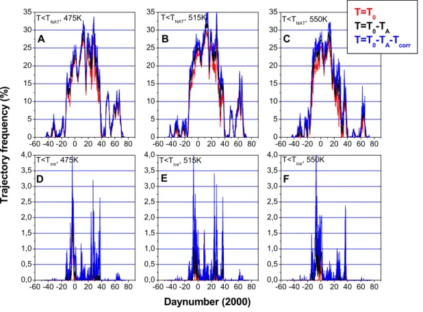
Initially, the influence of mountain waves on the tempera-tures is examined by analysing the trajectory data and deter-mining the percentage of the trajectories where the temper-ature drops below either TN AT or Tice as a function of day
number. This provides an estimate of the amount of trajecto-ries where NAT or ice particles can possibly exist. In Fig. 10 these percentages are shown for three different model lay-ers. An ample amount of trajectories is seen to have temper-atures below TN AT even without the presence of mountain
waves (panels A, B, C, red curves). However, the percent-age of trajectories where T <TN AT increases as mountain
wave effects are taken into consideration (panels A, B, C, black and blue curves), with the highest trajectory frequen-cies adhering to the strongest possible temperature pertur-bation (T =T0−TA−Tcorr, panels A, B, C, blue curves). In
the case of trajectories where T <Tice(panels D, E, F) only a
small amount of trajectories fulfills this criterion when moun-tain wave effects are not taken into consideration. In this case, temperatures below Tice are only observed briefly just
before day 0 and just before day 30 and 40 (panels D, E, F, red curves). When mountain wave-induced temperature fluctuations are included the number of trajectories where
T <Ticeincreases and temperatures below Tice are seen over
extended periods of time during the winter season, although the numbers typically are small (<0.5%), with the highest values reaching around 4% (panels D, E, F, black and blue curves). Again, the highest trajectory frequencies are ob-served in the case where the strongest possible temperature
-60 -40 -20 0 20 40 60 80 0 5 10 15 20 25 30 35 -60 -40 -20 0 20 40 60 80 0,0 0,5 1,0 1,5 2,0 2,5 3,0 3,5 4,0 -60 -40 -20 0 20 40 60 80 0 5 10 15 20 25 30 35 -60 -40 -20 0 20 40 60 80 0,0 0,5 1,0 1,5 2,0 2,5 3,0 3,5 4,0 -60 -40 -20 0 20 40 60 80 0 5 10 15 20 25 30 35 -60 -40 -20 0 20 40 60 80 0,0 0,5 1,0 1,5 2,0 2,5 3,0 3,5 4,0 A T<TNAT, 475K D Daynumber (2000) Tr a je c tor y f re que nc y ( % ) T<T ice, 475K B T<T NAT, 515K E T<Tice, 515K C T<T NAT, 550K F T<T ice, 550K T=T 0 T=T0-TA T=T0-TA-Tcorr
Fig. 10. Percentage of trajectories where the temperature is below either TN AT (top row) or Tice (bottom row) for three different model layers, 475 K, 515 K, and 550 K. Results are shown for three different temperature scenarios according to the colour coding, one without mountain wave pertubations and two where increasingly stronger mountain wave pertubations are included.
perturbation is employed (panels D, E, F, blue curves). As mentioned earlier, these results can only provide an estimate of the possible existence of NAT and ice particles. In order to evaluate the actual load of NAT and ice particles one must examine the outcome of the full microphysical simulation.
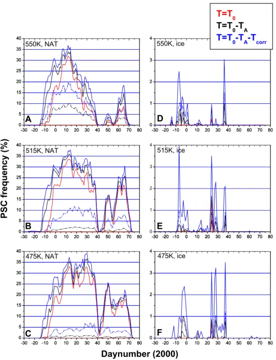
The percentage of trajectories containing NAT or ice par-ticles within the polar vortex as a function of day number ac-cording to the microphysical simulation is shown in Fig. 11. Results are shown for three different temperature scenarios and for two different choices of microphysics. In the present analysis, a trajectory is said to contain ice or NAT if the vol-ume density of these particle types exceeds zero. This is a very liberal definition of the presence of ice or NAT and should be interpreted as an upper limit. In the case of NAT (panels A, B, C), it is seen that NAT forms readily as a con-sequence of the synoptic conditions alone when NAT nucle-ation above Ticeis allowed (panels A, B, C, solid red curves).
When this is not the case no NAT particles are seen (panels A, B, C, dotted red curves). When mountain wave effects are included the period during which NAT particles are seen (panels A, B, C, black and blue curves) starts earlier in the winter compared to the case where mountain wave effects were not included (panels A, B, C, red curves). In the cases
where mountain wave effects are taken into account NAT is readily seen throughout the winter, regardless of the choice of microphysics, although the percentage of trajectories con-taining NAT is consistently higher in the case where NAT nucleation above Ticeis included.
The importance of mountain wave effects for NAT forma-tion seems much larger in the hemispheric simulaforma-tions than in the local ones. This could be because the synoptic temper-atures alone are generally well below TN AT in the local scale
simulations. If the additional cooling caused by mountain waves is not sufficient to lower the temperatures below Tice,
the addition of mountain wave effects will not cause many changes. Doing local scale model runs in relatively warmer periods (e.g. the early part of the winter) may reveal a greater impact of mountain waves on NAT formation on local scales as well.
Considering the ice particles (panels D, E, F) it is evident that, regardless of the choice of microphysics, practically no ice particles form as a consequence of the synoptic condi-tions alone (panels D, E, F, red curves), as was the case in the local-scale model runs as well. When mountain wave ef-fects are included the percentage of trajectories containing ice particles increases noticeably (panels D, E, F, black and
-30 -20 -10 0 10 20 30 40 50 60 70 80 0 5 10 15 20 25 30 35 40 -30 -20 -10 0 10 20 30 40 50 60 70 80 0 5 10 15 20 25 30 35 40 -30 -20 -10 0 10 20 30 40 50 60 70 80 0 1 2 3 4 -30 -20 -10 0 10 20 30 40 50 60 70 80 -30 -20 -10 0 10 20 30 40 50 60 70 80 0 1 2 3 4 -30 -20 -10 0 10 20 30 40 50 60 70 80 0 5 10 15 20 25 30 35 40 -30 -20 -10 0 10 20 30 40 50 60 70 80 0 1 2 3 4 -30 -20 -10 0 10 20 30 40 50 60 70 80 0 5 10 15 20 25 30 35 40 -30 -20 -10 0 10 20 30 40 50 60 70 80 0 1 2 3 4 -30 -20 -10 0 10 20 30 40 50 60 70 80 0 5 10 15 20 25 30 35 40 -30 -20 -10 0 10 20 30 40 50 60 70 80 0 1 2 3 4 -30 -20 -10 0 10 20 30 40 50 60 70 80 0 5 10 15 20 25 30 35 40
B
A
F
E
D
C
Daynumber (2000)
475K, ice 515K, NAT 515K, ice 550K, NAT 550K, iceT=T
0T=T
0-T
AT=T
0-T
A-T
corr 475K, NATFig. 11. Percentage of trajectories containing NAT (left column) and ice (right column) particles within the polar vortex as a function of
daynumber for the winter 1999-2000. Results are shown for three different model layers, 475 K, 515 K, and 550 K, and for three different temperature scenarios according to the colour coding, one without mountain wave pertubations and two where increasingly stronger mountain wave pertubations are included. The solid lines are from a series of simulations where NAT nucleation above Ticeis allowed whereas the dotted lines are from a simulation sequence where this is not the case.
blue curves), and trajectories containing ice particles are ob-served throughout the winter season. When NAT nucleation above Ticeis included (solid curves) the percentage is higher
than in the case where NAT nucleation above Ticeis not
al-lowed (dotted curves). These results are in agreement with the findings of D¨ornbrack and Leutbecher (2001) who found that practically all ice particle formation over Scandinavia was a consequence of mountain wave activity.
As seen above the effect of localised mountain wave ef-fects may extend beyond their local scale. In hemispheric model runs where mountain wave effects have been included NAT particle production is seen to increase and practically all the ice particles produced in the simulations can be directly attributed to the effect of mountain waves.
5 Results and discussion
Detailed model runs matching lidar measurements from two specific flight days (23 and 25 January 2000) of the NASA DC-8 during SOLVE/THESEO 2000 have been analysed and the correspondence between model data and observational data has been examined. Considering a quantitative analysis of the percentage of data points containing PSC 1a or PSC 2 the correspondence is better when NAT nucleation above
Tice is allowed than when this is not the case. In the case
of the local scale model runs the amount of PSC 1a is only slightly affected by the inclusion of mountain wave effects in the simulations, whereas mountain waves have a notice-able impact on the amount of PSC 2. In the latter case, the correspondence between measurements and model data in-creases greatly when mountain waves are added. The limited effect of mountain waves on NAT formation in the two sets of examined DC-8 data may be due to the fact that the syn-optic temperatures alone are rather low; substantial amounts of NAT are seen as a consequence of the synoptic conditions alone. Any additional cooling is not likely to result in signifi-cant changes unless the cooling results in temperatures below
Tice. In a series of sensitivity tests the qualitative differences
between the different microphysical scenarios were not af-fected by variations in the initial HNO3profile of ±1 ppbv.
In the case of large-scale model runs the effect of moun-tain waves on the solid particle production within the entire northern polar vortex over the course of the winter season 1999–2000 was shown to be quite significant: Practically no ice particles were seen as a consequence of the synoptic con-ditions alone whereas ice was observed for extended periods of time over the course of the winter when mountain wave ef-fects were taken into consideration, regardless of the choice of microphysics. However, the case where NAT nucleation above Tice was included consistently showed a higher
per-centage of trajectories containing ice particles. When NAT nucleation above Ticewas included the highest percentage of
trajectories containing ice particles were around 4%, whereas the percentage of ice particles is the case where NAT nu-cleation above Tice was not included did not exceed 0.5%,
see Fig. 11. NAT particles were seen to form readily as a consequence of the synoptic conditions alone, regardless of the choice of microphysics. However, with the inclusion of mountain wave effects the time period during which NAT particles were present became longer. As was the case with the ice particles, the percentage of trajectories containing NAT particles is greater when NAT nucleation above Tice
was included (up to 35% of the trajectories) than when this was not the case (up to 20% of the trajectories). Consider-ing the hemispheric simulations mountain wave effects seem to have a quite significant influence on the NAT formation, raising the percentage of trajectories containing NAT parti-cles by approximately 10% from the warmest to the coldest temperature scenario, see Fig. 11. This is contrary to what was seen in the two local-scale simulations matching
DC-8 flights examined here. A possible explanation could be that the synoptic temperatures alone were low enough to al-low for NAT formation during these two flights. Additional local-scale model runs from relatively warmer flight dates (e.g. early in the winter) could help shed some more light on this.
Given the large effect mountain waves apparently had on ice and NAT formation on hemispheric scales during the win-ter 1999–2000, the inclusion of mountain waves in models seems important in order to be able to provide accurate esti-mates of the PSC load within the vortex. It would be most interesting to determine whether or not the impact of moun-tain waves is as pronounced in other winters as well and such an examination is planned for a future study along with a series of comparisons between hemispheric model data and satellite observations.
6 Conclusions
Detailed lidar measurements of PSCs made by the NASA DC-8 have been compared to corresponding model runs from a microphysical PSC model using a number of different tem-perature and microphysical scenarios. It is found that the best agreement between measurements and model data is seen in the case where mountain wave effects are taken into consid-eration and where NAT nucleation above Tice is included in
the microphysics. Motivated by these findings the effect of the choice of microphysics and mountain waves on hemi-spheric PSC production is examined in a series of vortex-covering model runs extending over the 1999–2000 Arctic winter season. It is seen that the localised mountain wave-induced temperature perturbations have an effect on the pro-duction of solid PSCs which extend beyond their local scale; in the hemispheric model runs the percentage of trajecto-ries containing solid PSC particles increases when mountain wave effects are taken into account. Depending on the choice of microphysics, the inclusion of mountain waves is crucial. When NAT nucleation above Tice is not included in the
mi-crophysics, practically no trajectories containing ice or NAT particles are observed as a consequence of the synoptic con-ditions alone, whereas both particle types are seen to form when mountain wave effects are taken into consideration. When NAT nucleation above Tice is included in the
micro-physics, NAT particles can form as a result of the synoptic conditions alone. However, the amount of NAT and ice par-ticles increases as mountain wave effects are taken into con-sideration and the percentage of trajectories containing either NAT or ice is consistently larger in the scenario where NAT nucleation above Tice is included in the microphysics
Acknowledgements. Part of this work was carried out as part
of the EU-funded research project MAPSCORE (EVK2-CT-2000-00077). The Danish Research Council (SNF) is gratefully acknowledged for financial support. Support of the DC-8 lidar measurements was provided by the NASA Upper Atmospheric Research Program. MWFM-2 runs were partially supported by NASA’s Atmospheric Chemistry and Analysis Program and by the Office of Naval Research. The constructive criticism given by two anonymous referees is greatly appreciated.
Edited by: T. Koop
References
Biele, J., Tsias, A., Luo, B., Carslaw, K., Neuber, R., Beyerle, G., and Peter, T.: Nonequilibrium coexistence of solid and liquid particles an Arctic stratospheric clouds, J. Geophys. Res., 106, 22 991–23 007, doi:10.1029/2001JD00188, 2001.
Brogniez, C., Huret, N., Eckermann, S., Rivi`ere, E., Pirre, M., He-man, M., Balois, J.-Y., Verwaerde, C., Larsen, N., and Knudsen, B.: Polar stratospheric cloud microphysical properties measured by the microRADIBAL instrument on 25 January 2000 above Es-range and modeling interpretation, J. Geophys. Res., 108, 8332, doi:10.1029/2001JD001017, 2003.
Browell, E.: Differential absorption lidar sensing of ozone, Pro-ceedings of the IEEE, 77, 419–432, 1989.
Browell, E., Butler, C., Ismail, S., Robinette, P., Carter, A., Hig-don, N., Toone, O., Schoeberl, M., and Tuck, A.: Airborne Lidar Observations in the Wintertime Arctic stratosphere: Polar Strato-spheric Clouds, Geophys. Res. Lett., 17, 385–388, 1990. Carslaw, K. S., Wirth, M., Tsias, A., Luo, B., D¨ornbrack, A.,
Leut-becher, M., Volkert, H., Renger, W., Bacmeister, J., and Peter, T.: Particle microphysics and chemistry in remotely observed moun-tain polar stratospheric clouds, J. Geophys. Res., 103, 5785– 5796, 1998a.
Carslaw, K. S., Wirth, M., Tsias, A., Luo, B., D¨ornbrack, A., Leut-becher, M., Volkert, H., Renger, W., Bacmeister, J., Reimer, E., and Peter, T.: Increased stratospheric ozone depletion due to mountain-induced atmospheric waves, Nature, 391, 675–678, 1998b.
Carslaw, K. S., Peter, T., Bacmeister, J., and Eckermann, S.: Widespread solid particle formation by mountain waves in the Arctic stratosphere, J. Geophys. Res., 104, 1827–1836, 1999. Coffey, M., Mankin, W. G., and Hannigan, J. W.: Airborne
spec-troscopic observations of chlorine activation and denitrification of the 1999/2000 winter Arctic stratosphere during SOLVE, J. Geophys. Res., 108, 8303, doi:10.1029/2001JD001085, 2002. D¨ornbrack, A. and Leutbecher, M.: Relevance of mountain waves
for the formation of polar stratospheric clouds over Scandinavia: A 20 year climatology, J. Geophys. Res., 106, 1583–1593, 2001. Drdla, K., Schoeberl, M., and Browell, E.: Microphysical mod-elling of the 1999–2000 Arctic winter: 1. Polar stratospheric clouds, denitrification, and dehydration, J. Geophys. Res., 107, 8312, doi:10.1029/2001JD000782, 2002 (printed 108(D5), 2003).
Eckermann, S. D. and Preusse, P.: Global Measurements of Strato-spheric Mountain Waves from Space, Science, 286, 1534–1537, 1999.
Fueglistaler, S., Buss, S., Luo, B., Wernli, H., Flentje, H., Hostetler, C., Poole, L., Carslaw, K., and Peter, T.: Detailed modeling of mountain wave PSCs, Atmos. Chem. Phys., 3, 697–712, 2003,
SRef-ID: 1680-7324/acp/2003-3-697.
Gille, J. C. and Russell, J. M.: The Limb Infrared Monitor of the Stratosphere: Experiment Description, Performance, and Re-sults, J. Geophys. Res., 89, 5125–5140, 1984.
Hanson, D. and Mauersberger, K.: Laboratory studies of the ni-tric acid tryhydrate: Implications for the south polar stratosphere, Geophys. Res. Lett., 15, 855–858, 1988.
Hertzog, A., Vial, F., D¨ornbrack, A., Eckermann, S., Knud-sen, B., and Pommereau, J.-P.: In situ observations of grav-ity waves and comparisons with numerical simulations during the SOLVE/THESEO 2000 campaign, J. Geophys. Res., 107, doi:10.1029/2001JD001025, 2002.
Hitchman, M., McKay, M., and Trepte, C.: A climatology of stratospheric aerosol, J. Geophys. Res., 99, 20 689–20 700, doi:10.1029/94JD01525, 1994.
Hu, R.-M., Carslaw, K., Hostetler, C., Poole, L., Luo, D., Peter, T., F¨uglistaler, S., McGee, T., and Burris, J.: Microphysical proper-ties of wave polar stratospheric clouds retrieved from lidar mea-surements during SOLVE/THESEO 2000, J. Geophys. Res., 107, doi:10.1029/2001JD001125, 2002.
Irie, H., Pagan, K., Tabazadeh, A., Legg, M., and Sugita, T.: In-vestigation of polar stratospheric cloud solid particle formation mechanisms using ILAS and AVHRR observations in the Arctic, Geophys. Res. Lett., 31, L15107, doi:10.1029/2004GL020246, 2004.
Jiang, J., Eckermann, S., Wu, L., and Ma, J.: A search for moun-tain waves in MLS stratospheric limb radiance from the Northern Hemisphere: data analysis and global mountain wave modeling, J. Geophys. Res., 109, doi:10.1029/2003JD003974, 2004. Knopf, D., Koop, T., Luo, B., Weers, U., and Peter, T.:
Homo-geneous Nucleation of N AD and N AT in Liquid Stratospheric Aerosols: Insufficient to Explain Denitrification, Atmos. Chem. Phys., 2, 207–214, 2002,
SRef-ID: 1680-7324/acp/2002-2-207.
Knudsen, B. and Grooss, J.-U.: Northern mid-latitude stratospheric ozone dilution in spring modeled with simulated mixing, J. Geo-phys. Res., 105, 6885–6890, doi:10.1029/1999JD901076, 2000. Koop, T., Luo, B., Tsias, A., and Peter, T.: Water activity as the de-terminant for homogeneous ice nucleation in aqueous solutions, Nature, 406, 611–614, 2000.
Larsen, N.: Polar Stratospheric Clouds: A Microphysical Simula-tion Model, Scientific Report 91-2, Danish Meteorological Insti-tute, 1991.
Larsen, N.: Polar Stratospheric Clouds, Microphysical and Optical Models, Scientific report 00-06, Danish Meteorological Institute, 2000.
Larsen, N., Knudsen, B., Gauss, M., and Pitari, G.: Aircraft induced effects on Arctic polar stratospheric cloud formation, Meteorol-ogische Zeitschrift, 11, 207–214, 2002.
Larsen, N., Knudsen, B., Svendsen, S., Deshler, T., Rosen, J., Kivi, R., Weisser, C., Schreiner, J., Mauersberger, K., Cairo, F., Ovar-lez, J., Oelhaf, H., and Spang, R.: Formation of solid particles in synoptic-scale Arctic PSCs in early winter 2002/2003, Atmos. Chem. Phys., 4, 2001–2013, 2004,
Luo, B., Carslaw, K., Peter, T., and Clegg, S.: Vapour pressures of H2SO4/HNO3/HCl/HBr/H2O solutions to low stratospheric
temperatures, Geophys. Res. Lett., 22, 247–250, 1995.
Marti, J. and Mauersberger, K.: A survey and new measurements of ice vapor pressure at temperatures between 170 and 250 K, Geophys. Res. Lett., 20, 363–366, 1993.
Morcrette, J.-J.: Radiation and cloud radiative properties in the ECMWF operational weather forecast model, J. Geophys. Res., 96, 9121–9132, 1991.
Newman, P. A., Harris, N., Adriani, A., Amanatidis, G., Anderson, J., Braathen, G., Brune, W., Carslaw, K., Craig, M., DeCola, P., Guirlet, M., Hipskind, S., Kurylo, M., K¨ullmann, H., Larsen, N., M´egie, G., Pommereau, J.-P., Poole, L., Schoeberl, M., Stroh, F., Toon, O., Trepte, C., and Van Roozendael, M.: An overview of the SOLVE/THESEO 2000 campaign, J. Geophys. Res., 107, 8259, doi:10.1029/2001JD001303, 2002.
Ovarlez, J., Ovarlez, H., Crespin, J., and Gaubicher, B.: Water vapour measurements in the northern polar vortex, in: Compre-hensive Investigations of Polar Stratospheric Aerosols, CIPA Fi-nal Report, DMI Scientific Report 04-01, Danish Meteorological Institute, 2004.
Pagan, K., Tabazadeh, A., Drdla, K., Hervig, M., Eckermann, S., Browell, E., Legg, M., and Foschi, P.: Observational evidence against mountain-wave generation of ice nuclei as a prerequi-site for the formation of three solid nitric acid polar stratospheric clouds observed in the Arctic in early December 1999, J. Geo-phys. Res., 109, D04312, doi:10.1029/2003JD003846, 2004. Pierce, R., Al-Saadi, J., Fairlie, T., Natarajan, M., Harvey, V., Grose,
W., Russel, J., Bevilacqua, R., Eckermann, S., Fahey, D., Popp, P., Richard, E., Stimpfle, R., Toon, G., Webster, C., and Elkins, J.: Large-Scale Chemical Evolution of the Arctic Vortex Dur-ing the 1999–2000 Winter: HALOE/POAM3 Lagrangian Photo-chemical Modeling for the SAGE III Ozone Loss and Validation Experiment (SOLVE) Campaign, J. Geophys. Res., 108, 8317, doi:10.1029/2001JD001063, 2003.
Pinnick, T., Rosen, J., and Hofmann, D.: Stratospheric aerosol mea-surements III: Optical model calculations, J. Atmos. Sci., 33, 304–314, 1976.
Schreiner, J., Voigt, C., Kohlmann, A., Mauersberger, K., Deshler, T., Kroger, C., Larsen, N., Adriani, A., Cairo, F., Di Donfrancesco, G., Ovarlez, J., Ovarlez, H., and D¨ornbrack, A.: Chemical, microphysical, and optical proper-ties of polar stratospheric clouds, J. Geophys. Res., 108, 8313, doi:10.1029/2001JD000825, 2003.
Tabazadeh, A., Djikaev, Y., Hamill, P., and Reiss, H.: Laboratory Evidence for Surface Nucleation of Solid Polar Stratospheric Cloud Particles, J. Phys. Chem. A, 106, 10 238–10 246, 2002. Tolbert, M. A. and Toon, O. B.: Solving the PSC mystery, Science,
292, 61–63, 2001.
Toon, O. B., Tabazadeh, A., Browell, E., and Jordan, J.: Analysis of lidar observations of Arctic polar stratospheric clouds during January 1989, J. Geophys. Res., 105, 20 589–20 615, 2000. Voigt, C., Schreiner, J., Kohlmann, A., Zink, P., Mauersberger, K.,
Larsen, N., Deshler, T., Kr¨oger, C., Rosen, J., Adriani, A., Cairo, F., Di Donfrancesco, G., Viterbini, M., Ovarlez, J., Ovarlez, H., David, C., and D¨ornbrack, A.: Nitric Acid Trihydrate (NAT) in Polar Stratospheric Clouds, Science, 290, 1756–1758, 2000. WMO: Scientific Assessment of Ozone Depletion: 1998, Global
Ozone Research and Monitoring Project – Report No. 44, World Metorological Organization, 1999.