Sensitivity of tracer transport to model resolution, forcing data and tracer lifetime in the general circulation model ECHAM5

(1)

HAL Id: hal-00303227

https://hal.archives-ouvertes.fr/hal-00303227

Submitted on 8 Jan 2008

HAL is a multi-disciplinary open access

archive for the deposit and dissemination of sci-entific research documents, whether they are pub-lished or not. The documents may come from teaching and research institutions in France or abroad, or from public or private research centers.

L’archive ouverte pluridisciplinaire HAL, est destinée au dépôt et à la diffusion de documents scientifiques de niveau recherche, publiés ou non, émanant des établissements d’enseignement et de recherche français ou étrangers, des laboratoires publics ou privés.

Sensitivity of tracer transport to model resolution,

forcing data and tracer lifetime in the general

circulation model ECHAM5

A. Aghedo, S. Rast, M. G. Schultz

To cite this version:

A. Aghedo, S. Rast, M. G. Schultz. Sensitivity of tracer transport to model resolution, forcing data and tracer lifetime in the general circulation model ECHAM5. Atmospheric Chemistry and Physics Discussions, European Geosciences Union, 2008, 8 (1), pp.137-160. �hal-00303227�

(2)

ACPD

8, 137–160, 2008 Sensitivity of tracer transport in ECHAM5 A. M. Aghedo et al. Title Page Abstract Introduction Conclusions References Tables Figures ◭ ◮ ◭ ◮ Back Close

Full Screen / Esc

Printer-friendly Version

Interactive Discussion

EGU Atmos. Chem. Phys. Discuss., 8, 137–160, 2008

www.atmos-chem-phys-discuss.net/8/137/2008/ © Author(s) 2008. This work is licensed

under a Creative Commons License.

Atmospheric Chemistry and Physics Discussions

Sensitivity of tracer transport to model

resolution, forcing data and tracer lifetime

in the general circulation model ECHAM5

A. Aghedo1, S. Rast1, and M. G. Schultz2

1

Max Planck Institute for Meteorology, Hamburg, Germany

2

ICG-2, Research Centre, J ¨ulich, Germany

Received: 13 November 2007 – Accepted: 5 December 2007 – Published: 8 January 2008 Correspondence to: A. M. Aghedo (adetutu.aghedo@gmail.com)

(3)

ACPD

Full Screen / Esc

EGU

Abstract

The transport of tracers in the general circulation model ECHAM5 is analysed using 9 independent idealized tracers with constant lifetimes released in different altitude regions of the atmosphere. The source regions were split into the tropics, Northern and Southern Hemisphere. The dependency of tracer transport on model resolution is

5

tested in the resolutions T21L19, T42L19, T42L31, T63L31 and T106L31, by employ-ing tracers with a globally uniform lifetime of 5 months. Each of the experiments uses prescribed sea surface temperatures and sea ice fields of the 1990s. The influence of meteorology and tracer lifetimes were tested by performing additional experiments in the T63L31 resolution, by nudging ECHAM5 towards the European Centre for Medium

10

Range Weather Forecast 40 years re-analysis data (ERA40), and by using tracer life-times of 0.5 and 50 months, respectively. The transport of tracers is faster in the finer resolution models and is mostly dependent on the number of vertical levels. We found a decrease in the inter-hemispheric transport of tracers with source region at the sur-face or the tropopause in the coarse resolution models due to increasing recirculation

15

within the source region and vertical mixing. However, a coarse model resolution leads to enhanced inter-hemispheric transport in the stratosphere. The use of ERA40 data only slightly affects the inter-hemispheric transport of surface and tropopause tracers, whereas it increases the inter-hemispheric and vertical transport in the stratosphere by up to 100% and by a factor of 2.5, respectively. The inter-hemispheric transport time

20

was deduced from simulations with tracers of infinite lifetime and source regions at the surface in the Northern and Southern Hemisphere. Again, the transport was found to be faster for models with higher vertical resolution. We find inter-hemispheric transport times of about 7 to 9 months which are lower than the values reported in the literature, based for example on85Kr observations.

(4)

ACPD

Full Screen / Esc

EGU

1 Introduction

Transport plays a crucial role in determining the distribution of gas-phase and par-ticulate trace constituents in the atmosphere. Numerical models are an essential tool for simulating atmospheric transport and distribution of trace species. How-ever, the ability of a model to simulate the observed distributions of these trace

5

species is largely dependent on its capability to reproduce the transport and mixing of the real atmosphere. Gurney et al. (2002, 2003) show that differences in model transport are a significant source of uncertainty. Hall et al. (1999) concluded that transport inaccuracies significantly affect the simulation of important long-lived trace species in the lower stratosphere. Model resolution also plays an important role.

10

Genthon and Armengaud(1995) hinted that model spatial resolution is an important factor in the simulation of the distribution of 222Rn, while Austin et al. (1997) and Wild and Prather(2006) demonstrated the influence of model resolution on the sim-ulation of ozone distribution in the stratosphere and the troposphere, respectively.

Idealized tracers have previously been employed to investigate specific features of

15

atmospheric transport, for exampleGray(2003) used passive tracers to study the influ-ence of convection on stratosphere – troposphere exchange of air. Also by comparing the results from different model resolutions, idealized tracers may explain some of the discrepancies observed in the distribution or seasonality of atmospheric trace species in different models (e.g.Genthon and Armengaud,1995;Jacob et al.,1997;Denning

20

et al.,1999;Stevenson et al.,2006).

In a special issue of the Journal of Climate, titled “Climate Models at the Max Planck Institute for Meteorology (MPI-M)” (Vol. 19, Issue 16, August 2006), the influence of model resolution on simulated climate in the ECHAM5 (Roeckner et al., 2003) gen-eral circulation model (GCM) was presented byRoeckner et al.(2006). The evaluation

25

of the hydrological cycle in the model is presented byHagemann et al. (2006). The snow cover and surface albedo were assessed inRoesch and Roeckner(2006), while Wild and Roeckner(2006) discussed the radiative fluxes in the model. This study

(5)

ex-ACPD

Full Screen / Esc

EGU tends the assessment of the ECHAM5 model by testing the sensitivity of the

trans-port of tracers “emitted” at 9 different locations in the model, in order to answer three major questions: (1) How sensitive is the transport of tracers to model resolution? (2) How does a change in forcing meteorology and tracer lifetime affect tracer trans-port? (3) What are the characteristic time scale for inter-hemispheric transtrans-port?

5

A brief description of the ECHAM5 model and the details of the model set-up are given in Sect.2. The results are presented in Sect. 3 through 5. These include the analysis of the global characteristics of tracer transport in Sect. 3, the discussion of the transport from the source regions into various receptor regions in Sect.4, and the calculation of the inter-hemispheric transport time in Sect. 5. The summary of our

10

findings is presented in Sect.6.

2 Model description

2.1 The ECHAM5 general circulation model

The atmospheric general circulation model ECHAM5 is the fifth-generation cli-mate model developed at the Max Planck Institute for Meteorology, evolving

orig-15

inally from the model of the European Centre for Medium-range Weather Forecast (ECMWF) (Simmons et al.,1989). The dynamical core of ECHAM5 solves prognos-tic equations for vorprognos-ticity, divergence, logarithm of surface pressure and temperature, which are expressed in the horizontal by spectral coefficients. The model uses a semi-implicit leapfrog time integration scheme (Robert et al.,1972;Robert,1981,1982) and

20

a special time filter (Asselin, 1972). The vertical axis uses a hybrid terrain-following sigma-pressure coordinate system and finite-difference scheme citepsimbur81. The finite-difference scheme is implemented such that energy and angular momentum are conserved. Water vapour, cloud liquid water, cloud ice and trace components are trans-ported with a flux form semi-Lagrangian transport scheme (Lin and Rood,1996) on a

25

(6)

ACPD

Full Screen / Esc

EGU ECHAM5 contains a microphysical cloud scheme (Lohmann and Roeckner,1996)

with prognostic equations for cloud liquid water and ice. Cloud cover is predicted with a prognostic-statistical scheme solving equations for the distribution moments of total water (Tompkins,2002). Convective clouds and convective transport are based on the mass-flux scheme of Tiedtke (1989) with modifications based onNordeng(1994). A

5

detailed model description is given inRoeckner et al.(2003). The model successfully participated in recent scenario experiments for the fourth assessment report of the Intergovernmental Panel on Climate Change.

ECHAM5 can be run as a coupled ocean-atmosphere model, or with forced bound-aries from prescribed sea surface temperatures and sea ice cover fields. In addition,

10

a Newtonian relaxation technique, also termed “nudging” (Hoke and Anthes, 1976; Jeuken et al.,1996) can be applied in order to simulate real weather episodes. The atmospheric forcing (surface pressure, temperature, vorticity, and divergence) is then obtained from numerical weather prediction models with data assimilation, e.g. the ECMWF 40-years re-analysis data (ERA40,Simmons and Gibson,2000).

15

ECHAM5 contains a flexible software structure for definining atmospheric tracers. These tracers are then subjected to advection, convection and vertical diffusion. These transport processes are calculated separately using an operator splitting method. In ECHAM5, advective transport is done first, followed by vertical diffusion, chemical re-actions or exponential decay, and in a last step convective transport. Each transport

20

process is calculated from the knowledge of the tracer concentration at the preceding time step except the convection in which the tracer concentration updated by the previ-ous processes is used. The resulting tendencies of each single process are added to the concentration of the previous time step. This operator splitting is different from the classical strang splitting which was discussed inLanser and Verwer(1999).

25

2.2 Experiment description

We consider nine independent idealized tracers each constrained to have constant mass mixing ratio of 1 in their respective source regions (see Fig.1). This is equivalent

(7)

ACPD

Full Screen / Esc

EGU to prescribing a source which is proportional to the temporally varying outflow from the

region.

Horizontally, we divide the earth surface into three equal-area latitude bands called “north” (N), “tropics” (T) and “south” (S), followingBowman and Carrie(2001);Bowman and Erukhimova (2004). “North” refers to the region north of 19◦N, the region south

5

of 19◦S is “south” and the region in the latitude bands in-between 19◦N and 19◦S is “tropics”. Vertically we introduce the tracers at three different altitude regimes (i.e. “sur-face”, “tropopause” and “stratosphere”). The “surface” tracers have their source at the lowest model level. The “tropopause” tracers have their source in the tropopause re-gion, which is assumed to correspond to model levels at 100 hPa in the T region and

10

200 hPa elsewhere. The “stratosphere” tracers have their source at the model level that corresponds to 30 hPa, which is the second level in the vertical resolutions L19 and L31 used in the simulations. Henceforth, we will abbreviate the tracer names by combin-ing their vertical and horizontal source region names; for example surfT is the surface tracer with source region in the tropics, while tropN stands for the tracer which is kept

15

at constant concentration in the Northern-Hemisphere tropopause region (see Fig.1). All tracers decay with a fixed globally uniform lifetime which is normally 5 months.

The experiments in this study are performed using a setup similar to the Atmospheric Model Intercomparison Project 2 (AMIP2,Gates et al.,1999) with prescribed sea sur-face temperatures and sea ice climatologies of the 1990s. Experiments to test the

20

resolution dependency of tracer transport were performed in the resolutions T21L19, T42L19, T42L31, T63L31, and T106L31. The simulations were run in each resolution for 5 years including 1-year spin-up time.

Additional sensitivity experiments were performed to test the influence of ERA40 meteorology (run T63L31-era40, using 5 months tracer lifetime) and to demonstrate the

25

influence of the tracer lifetimes. The latter runs were performed in T63L31 resolution with tracer lifetimes of 0.5 and 50 months, respectively. With a longer tracer lifetime, the model takes longer to reach a quasi steady state. Therefore, the 50 months lifetime experiment was run for a total of 13 years, of which we analyse the last 4 years.

(8)

ACPD

Full Screen / Esc

EGU The inter-hemispheric exchange time was investigated in experiments with tracers

of infinite lifetime. Thus, we assure that the tracers are not destroyed before they reach the other hemisphere.

3 The influence of model resolution on the global transport characteristics

The objective of this section is to characterise the resolution dependency of the export

5

flux of tracer from its source regioni into the global atmosphere. Across all the

resolu-tions, the tracer lifetimeτ is set as 5 months, which roughly corresponds to the lifetime

of CO in the troposphere.

For any given tracer with source in regioni and resolution r, the rate of change of

the global massM_i,r is given by:

10

˙

M_i,r(t) = Si ,r(t) −

M_i,r(t)

τ (1)

whereSi ,r is the time dependent mass flux out of the source regioni in the resolution

r.

According to our simulation setup, at t=0, Mi,r(0) equals the mass of the tracer

in the source region. This implies that Mi,r(0) is proportional to the source region

15

volume, because the tracer is uniformly distributed in the source region. The volume of the source region depends on the exact location of the grid box boundaries which demarcate the source region in each model resolution. Consequently, for each model resolutionr, we normalise the quantities in Eq. (1) by dividing them with M_i,r(0). With

m_i,r=Mi ,r/Mi,r(0) andsi ,r=Si ,r/Mi ,r(0), we get:

20

˙

m_i,r(t) = si,r(t) −

m_{i ,r}(t)

τ (2)

(9)

ACPD

Full Screen / Esc

Printer-friendly Version Interactive Discussion EGU a comparison index,R_{i ,r}: R_i,r(t) = mi,r(t) ˆ mi,T 63L31 (3)

Figure 2 displays the monthly mean values of Ri,r across the model resolutions.

Figure2 shows that most of the simulations reached a quasi steady state over the last 4-year period. Therefore the integration of the left hand side of Eq. (2) over the last

5

4 years of the simulations yields: Z

4 years ˙

m_i,r(t) d t = 0 (4)

This results in:

¯

si,r(t) =

¯

mi ,r(t)

τ (5)

where the bar indicates the 4-year average. This implies that the average export flux

10

from source regioni in resolution r is proportional to the global mass of tracer i in the

quasi steady state. Therefore the order of the curves in Fig.2directly corresponds to the strength of the export fluxes in the respective model resolution.

The Ri,r values of the tropopause and surface tracers in the 19-level (L19)

(i.e. T21L19 and T42L19) experiments lie below the curves of the 31-level (L31) runs.

15

Generally, there appears to be little influence of the horizontal resolution on global char-acteristics of tracer transport. A notable exception is the surfT tracer, which exhibits different values in the T21L19 and the T42L19 resolutions. To a lesser extent, the T106L31 resolution yields a largerR_i,r values than other 31-level simulations for the surfN and surfS tracers. The largest differences between the L19 and L31 resolutions

20

are found in the tropopause tracers. This can be explained by the position of the source regions relative to the tropopause.

(10)

ACPD

Full Screen / Esc

EGU Some of the tracers (i.e. stratS, stratT, stratN, surfS, and surfN) show a distinct

sea-sonal variation in all model resolutions, while others (i.e. tropS, tropN and surfT) exhibit only little variability. The tropT tracer has the least regular pattern, and it appears to follow a six-monthly seasonal cycle.

The relaxation of the atmospheric dynamics of the model to ERA40 data (i.e. run

5

T63L31-era40) yields values of R_{i ,r} which is about 10% higher for the stratosphere tracers and about 10–15% lower for the tropopause tracers. The surface tracers ex-hibit relatively small differences compared to the AMIP2 T63L31 simulation. In addi-tion, the T63L31-era40 run exhibits the Quasi Biennial Oscillation (QBO) in the stratT tracer. The presence of a QBO in this simulation is a consequence of the data

as-10

similation procedure used to generate the ERA40 data. The ECHAM5 model, as used for our experiments does not resolve the stratosphere and hence cannot sim-ulate the QBO, which could only be generated in the middle atmosphere ECHAM5 (MAECHAM5) model (Giorgetta et al.,2006).

An important feature for the application of the ECHAM5 model to chemistry transport

15

simulations (e.g. Aghedo et al., 2007) is the fact that there is little difference in the transport between the T42L31 and the finer T63L31 resolution. This is in contrast to Roeckner et al.(2006) who found an improvement of the zonal mean climate state for increased horizontal resolution, but little change between T42L19 and T42L31.

4 Source-receptor relationships 20

Table1 lists the fraction of tracer mass exported from source regioni into the

atmo-spheric column of the receptor regions S, T, and N in quasi steady state. It shows that the mean meridional transport of the surface and the tropopause tracers decreases in the coarse resolution models, except for the advection into the tropical region. This is a consequence of increased vertical mixing and recirculation in the coarse resolution

25

models (see discussion on Table2below). However, a coarser model resolution leads to an increase in the inter-hemispheric transport in the stratosphere (see Table1), with

(11)

ACPD

Full Screen / Esc

EGU the exception of stratT tracer transported into S region.

Constraining the model with ERA40 data generally lead to a small change of about 1–3% in the inter-hemispheric exchange of surface and tropopause tracers. In contrast to its influence at the surface and the tropopause, ERA40 data increases the inter-hemispheric transport in the stratosphere; this increase is about 9–15% for transport

5

from the tropical region to both hemispheres and about 100% for long-range exchange between the N and S regions. The QBO generated in the T63L31-era40 simulation may have contributed to this high inter-hemispheric mass exchange observed in the stratosphere tracers.

Table 1 also shows that the long-range inter-hemispheric exchange between the

10

Northern and the Southern Hemisphere, and the inter-hemispheric transport of strato-sphere tracers are most sensitive to the tracer lifetime. The largest differences occur between the tracers of 15 days and 5 months lifetime. The 50 months surface and tropopause tracers are well mixed, therefore the distribution within the regions varies by less than 7%, whereas this variation in the stratosphere tracers is up to 30%.

15

The cross tropopause transport of trace species plays a role for the budgets of vari-ous trace gases like ozone and halocarbons. As a proxy for cross tropopause transport, we consider the transport of the surface tracers to the stratosphere (i.e. the percent-age of surface tracers found above the 50 hPa level) and transport of the stratosphere tracers to below 750 hPa (Table2). The vertical transport of the tracers shows a

de-20

pendence on the number of vertical levels, and models with fewer vertical levels show larger vertical transport. The percentage amount of tropical surface tracer transported to the stratosphere is slightly higher than that transported from its corresponding N and S region, due to the influence of convection in the tropics. Also slightly higher vertical exchange is observed in the NH compared to the SH due to orographic effects.

25

Although ERA40 data have little effect on the vertical mixing of the surface trac-ers within the troposphere, it increases their vertical transport to the stratosphere by about a factor of 2.5 (Table 2). ERA40 data also increase the transport of strato-sphere tracers to below 750 hPa by up to 70%. This is consistent with findings of

(12)

ACPD

Full Screen / Esc

EGU Van Noije et al.(2004), who investigated the sensitivity of stratosphere-to-troposphere

exchange towards different meteorological forcing conditions in their chemistry trans-port model.

Owing to the long residence time of air in the stratosphere relative to our chosen lifetimes, the fraction of the mass exchanged between the stratosphere and the

tropo-5

sphere tends to 0 when the lifetime is short (0.5 month). The fraction of the surface trac-ers transported to above 50 hPa and stratosphere tractrac-ers transported to below 750 hPa rises respectively to about 0.4% and 1% when the lifetime is increased to 5 months, and to 4% and 15% when the lifetime increases to 50 months.

5 Inter-hemispheric transport time 10

In this section, we calculate the inter-hemispheric transport time between the Northern and Southern Hemispheres, by setting the boundary at the equator. This may be physically interpreted to represent the inter-tropical convergence zone (ITCZ) at the equator which acts as a major resistance to air mass exchange between Northern and Southern Hemispheres.

15

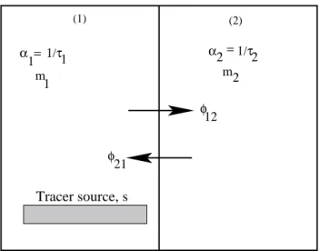
We use a conceptual two box-model, with one of the boxes containing the tracer sources as shown in Fig.3. For each boxi =1, 2, we denote the mass of tracer in the

respective box bymi. The decay rate of a tracer in box i is αi=1/τi, where τi is the

tracer lifetime. The transition rate of any tracer from boxi to box j , i6=j is φij=1/τij,

wherei, j=1, 2. For this general setting, the kinetic equations for the tracer mass are

20 as follows: ˙ m1= −α1m1−φ12m1+ φ21m2+ s (6) ˙ m2= −α2m2−φ21m2+ φ12m1 (7)

If a tracer with an infinite lifetime and no source (i.e. α1=α2=0, and s=0) attains a spatially uniform distribution in the steady state, it can be shown thatφ12=φ21=φ. If

25

(13)

ACPD

Full Screen / Esc

EGU a non-uniform distribution), we can calculate the seasonality of the inter-hemispheric

transport timeτex=1/φ from Eq. (7), noting thatα=0 when the tracer has infinite

life-time:

τ_ex = m1−m2 ˙

m2

(8)

This is the equation of Prather et al. (1987), which was also used by

5

Kjellstr ¨om et al.(2000) to determine the inter-hemispheric transport time from simu-lated SF6concentrations.

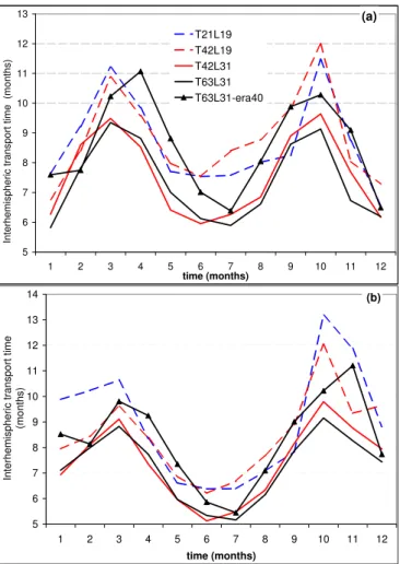
Figure 4shows the results of the inter-hemispheric transport time calculated using surfN and surfS tracers in the model resolutions T21L19, T42L19, T42L31, T63L31, and the T63L31-era40 version. The minima of the exchange time occur in the months

10

of December to January and June to July. During these months, the exchange of the air masses across the equator is particularly active and the transport times for tracers in both directions are low. This cycle is connected to the position of the ITCZ, which migrates to the north and south of the equator in July–August and January–February respectively, thereby allowing the air masses to easily cross the equator. Furthermore,

15

the more rapid the location of the ITCZ changes, the more intense is the associated exchange of air masses between the large scale northern and southern convective systems.

Figure4also shows that the inter-hemispheric exchange times of the finer resolution models in the AMIP2 runs are 1–2 months lower than those of the coarse resolution

20

models and T63L31-era40 simulation.

The annual mean values of the inter-hemispheric transport time across various model resolutions are given in Table 3. These results are lower than the inter-hemispheric exchange time of 1.5–1.7 years calculated from 85Kr concentrations byLevin and Hesshaimer(1996) with the use of a different two-box model. They explain

25

however, that their result may overestimate the real inter-hemispheric transport time because the interpolation of observation data neglects a decrease in concentration to-wards higher altitudes and in the stratosphere. We remark that the inter-hemispheric

(14)

ACPD

Full Screen / Esc

EGU exchange time of 1.14±0.16 yr estimated byCzeplak and Junge(1974) is shorter than

the exchange time ofLevin and Hesshaimer(1996) but still higher than our 0.60 to 0.74 years. Our new results for ECHAM5 are very similar to the seasonal variation of the inter-hemispheric exchange time calculated with ECHAM4 byKjellstr ¨om et al.(2000).

An analysis of the cross tropopause transport time is not possible within this

5

study, due to the wide range of transport time scales in the stratosphere and for the stratosphere-troposphere exchange.

6 Summary and conclusions

The influence of model resolution, ERA40 meteorology and the lifetime on the transport of tracers in ECHAM5 has been examined using 9 tracers defined at different horizontal

10

and vertical regions. Generally, transport is more vigorous in the finer resolution models and are mostly dependent on the number of vertical levels. The T42L31 resolution yields similar transport to other L31 simulations.

We found a decrease in the inter-hemispheric transport of surface and tropopause tracers in the coarse resolution models due to an increase in the vertical mixing and

15

recirculation within the source region. However, a coarse model resolution leads to enhanced inter-hemispheric transport in the stratosphere. The use of ERA40 data only slightly affects the inter-hemispheric transport of surface and tropopause tracers, whereas it increases the inter-hemispheric and vertical transport of tracers in the strato-sphere by up to 100%, and a factor of 2.5, respectively. The use of ERA40 data also

20

show the effect of Quasi-Biennial Oscillation on transport at the tropical stratosphere. The long-range inter-hemispheric transport between the Northern and the Southern Hemisphere, and the inter-hemispheric transport of the stratosphere tracers are most affected by the tracers’ lifetime. The largest differences are however found between the tracers with lifetime of 0.5 month and 5 months. The 50 months surface and tropopause

25

tracers are well mixed, therefore the distribution within the regions vary by less than 7%, and the percentage amount found in our 3-latitudinal regions is between 30–36% irrespective of their source region. Tracer lifetime also has a strong influence on the

(15)

ACPD

Full Screen / Esc

EGU seasonal cycle of the tracers.

The interpretation of the simulation results with a conceptual box model shows that it will take about 7 to 9 months for the surface tracer with source in the Southern and Northern Hemisphere respectively to be transported to the other hemisphere. These results are lower than the inter-hemispheric exchange time of 1.5–1.7 years calculated

5

from85Kr concentration byLevin and Hesshaimer(1996) with the use of a different two box model. The inter-hemispheric transport is most active in December to January and June to July. The finer resolution models in the AMIP2 runs yield a seasonal cycle of the inter-hemispheric exchange times, which are 1–2 months lower than those of the coarse resolution models and T63L31-era40 simulation.

10

Acknowledgements. This work was carried out during the doctoral work of AMA, sponsored by

the ZEIT foundation through the International Max Planck Research School on Earth System Modelling (IMPRS-ESM). S. Rast and M. G. Schultz acknowledge funding from the EU project RETRO (EVK2-CT-2002-00170). We are grateful to E. Roeckner for providing an in-house review of the manuscript, and to M. Giorgetta for his useful comments, and also to L. Kornblueh

15

for the technical assistance. The model runs were performed on the Sun Computing system (YANG) at the Max Planck Institute for Meteorology, Hamburg and the NEC SX-6 computer at the German Climate Computing Centre (“Deutsches Klimarechenzentrum”).

References

Aghedo, A. M., Schultz, M. G., and Rast, S.: The influence of African air pollution on regional

20

and global tropospheric ozone, Atmos. Chem. Phys., 7, 1193–1212, 2007,

http://www.atmos-chem-phys.net/7/1193/2007/. 145

Asselin, R.: Frequency filter for time integrations, Mon. Weather. Rev. 100, 487–490, 1972.140

Austin, J., Butchart N., and Swinbank, R.: Sensitivity of ozone and temperature to vertical resolution in a GCM with coupled stratospheric chemistry, Q. J. R. Meteorol. Soc., 123,

25

1405–1431, 1997. 139

Bowman, K. P. and Carrie, G. D.: The mean-meridional transport circulation of the troposphere in an idealized GCM, J. Atmos. Sci., 59, 1502–1514, 2001. 142

Bowman, K. P. and Erukhimova, T.: Comparison of global-scale Lagrangian transport proper-ties of the NCEP Reanalysis and CCM3, J. Climate, 17, 1135–1145, 2004. 142

(16)

ACPD

Full Screen / Esc

EGU

Czeplak, G. and Junge, C.: Studies of interhemispheric exchange in the troposphere by a diffusion model, Adv. Geophys., 18B, 57–72, 1974.149

Denning, A. S., Holzer, M., Gurney, K. R., et al.: Three-dimensional transport and concentration of SF₆: A model intercomparison study (TransCom 2), Tellus 51B, 266–297, 1999. 139

Gates, W. L., Boyle, J. S., Covey, C., Dease, C. G., Doutriaux, C. M., Drach, R. S., Fiorino, M.,

5

Gleckler, P. J., Hnilo, J. J., Marlais, S. M., Phillips, T. J., Potter, G. L., Santer, B. D., Sperber, K. R., Taylor, K. E., and Williams, D. N.: An Overview of the Results of the Atmospheric Model Intercomparison Project (AMIP I), B. Am. Meteorol. Soc., 80(1), pp. 2955, 1999. 142

Genthon, C. and Armengaud, A.: Radon 222 as a comparative tracer of transport and mixing in two general circulation models of the atmosphere, J. Geophys. Res., 100(D2), 2849–2866,

10

1995. 139

Giorgetta, M. A., Manzini, E., Roeckner, E., Esch, M., and Bengtsson, L.: Climatlogy and forcing of the quasi-biennial oscillation in the MAECHAM5 model, J. Climate, 19, 3882–3901, 2006.

145

Gray, S. L.: A case study of stratosphere to troposphere transport: The role of convective

15

transport and the sensitivity to model resolution, J. Geophys. Res., 108(D18), 4590, 2003.

139

Gurney, K. R., Law, R. M., Denning, A. S., et al.: Towards robust regional estimates of CO2 sources and sinks using atmospheric transport models, Nature, 415, 626–630, 2002. 139

Gurney, K. R., Law, R. M., Denning, A. S., et al.: TransCom 3 CO₂inversion intercomparison:

20

1. Annual mean control results and sensitivity to transport and prior flux information, Tellus 55B, 555–579, 2003. 139

Hagemann, S., Arpe, K., and Roeckner, E.: Evaluation of the Hydrological Cycle in the ECHAM5 Model, J. Climate, 19(16), 3810–3827, 2006. 139

Hall, T. M., Waugh, D. W., Boering, K. A., and Plumb, R. A.: Evaluation of transport in

strato-25

spheric models, J. Geophys. Res., 104(D15), 18 815–18 839, 1999. 139

Hoke, J. E. and Anthes, R. A.: The initialization of numerical models by a dynamic-initialization technique, Mon. Weather. Rev., 104(12), 1551–1556, 1976.141

Jacob, D. J., Prather, M. J., Rasch, P. J., et al.: Evaluation and intercomparison of global atmospheric transport models using222Rn and other short-lived tracers, J. Geophys. Res.,

30

102(D5), 5953–5970, doi:10.1029/96JD02955, 1997.139

Jeuken, A. B. M., Siegmund, P. C., Heijboer, L. C., Feichter, J., and Bengtson, L.: On the potential of assimilating meteorological analysis in a climate model for the purpose of model

(17)

ACPD

Full Screen / Esc

EGU

validation, J. Geophys. Res., 101, 16 939–16 950, 1996. 141

Kjellstr ¨om, E., Feichter, J., and Hoffman, G.: Transport of SF6 and 14

CO₂ in the atmospheric general circulation model ECHAM4, Tellus 52B, 1–18, 2000. 148,149

Lanser, D. and Verwer, J. G.: Analysis of operator splitting for advection-diffusion-reaction prob-lems from air pollution modelling, J. Comput. Appl. Math., 111, 201–216, 1999.141

5

Levin, I. and Hesshaimer, V.: Refining of atmospheric transport model entries by the globally observed passive tracer distribution of85Krypton and sulfur hexafluoride (SF₆), J. Geophys. Res., 101(D11), 16 745–16 755, 1996. 148,149,150

Lin, S.-J. and Rood, R. B.: Multidimensional Flux-Form Semi-Lagrangian Scheme, Mon. Weather. Rev., 124, 2046–2070, 1996.140

10

Lohmann, U. and Roeckner, E.: Design and performance of a new cloud microphysics scheme developed for the ECHAM general circulation model, Clim. Dynam., 12(8), 557–572, 1996.

141

Mesinger, F. and Arakawa, A.: Numerical methods used in atmospheric models, Global Atmo-spheric Research Programme (GARP) Publication Series, 17, World Meteorological

Organi-15

sation, 1976.140

Nordeng, T. E.: Extended versions of the convective parameterization scheme at ECMWF and their impact on the mean and transient activity of the model in the tropics. Technical memorandum No. 206, European Centre for Medium-range Weather Forecasts (ECMWF), Reading, United Kingdom, 1994. 141

20

Prather, M., McElroy, M., Wofsy, S., Russell, G., and Rind, D.: Chemistry of the global tropo-sphere: Fluorocarbons as tracers of air motion, J. Geophys. Res., 92, 6579–6613, 1987.

148

Robert, A. J.: A stable numerical integration scheme for the primitive meteorological equations, Atmos. Ocean., 19, 35–46, 1981. 140

25

Robert, A. J.: A semi-Lagrangian and semi-implicit numerical integration fscheme for the prim-itive meteorological equations, J. Met. Soc. Japan, 60, 319–325, 1982.140

Robert, A. J., Henderson, J., and Turnbull, C.: An implicit time integration scheme for baroclinic models in the atmosphere, Mon. Weather. Rev., 100, 329–335, 1972. 140

Roeckner, E., B ¨auml, G., Bonaventura, L., Brokopf, R., Esch, M., Giorgetta, M., Hagemann, S.,

30

Kirchner, I., Kornblueh, L., Manzini, E., Rhodin, A., Schlese, U., Schulzweida, U., and Tomp-kins, A.: The atmospheric general circulation model ECHAM 5. PART I: Model description, Max-Planck Institute for Meteorology, Report No. 349, Hamburg, Germany, 127pp, 2003.

(18)

ACPD

Full Screen / Esc

EGU

139,141

Roeckner, E., Brokopf, R., Esch, M., Giorgetta, M., Hagemann, S., Kornblueh, L., Manzini, E., Schlese, U., and Schulzweida, U.: Sensitivity of simulated climate to horizontal and vertical resolution in the ECHAM5 atmosphere model, J. Climate, 19, 3771–3791, 2006.139,145

Roesch, A. and Roeckner, E.: Assessment of Snow Cover and Surface Albedo in the ECHAM5

5

General Circulation Model, J. Climate, 19(16), 3828–3843, 2006. 139

Simmons, A. J., Burridge, D. M., Jarraud, M., Girard, C., and Wergen, W.: The ECMWF medium-range prediction models development of the numerical formulations and the impact of increased resolution, Meteorol. Atmos. Phys., 40, 28–60, doi:10.1007/BF01027467, 1989.

140

10

Simmons, A. J. and Burridge, D. M.: An energy and angular-momentum conserving vertical finite difference scheme and hybrid vertical coordinates, Mon. Weather. Rev., 109, 758–766, 1981.

Simmons, A. J. and Gibson, J. K.: ERA-40 Project plan. ERA40 project report series No 1, 63pp, 2000. 141

15

Stevenson, D. S., Dentener, F. J., Schultz, M. G., et al.: Multimodel ensemble simula-tions of present-day and near-future tropospheric ozone, J. Geophys. Res., 111, D08301, doi:10.1029/2005JD006338, 2006. 139

Tiedtke, M.: A comprehensive mass flux scheme for cumulus parameterization in large-scale models, Mon. Weather. Rev., 117, 1779–1800, 1989. 141

20

Tompkins, A. M.: A prognostic parameterization for the subgrid-scale variability of water vapour and clouds in large-scale models and its use to diagnose cloud cover, J. Atmos. Sci., 59, 1917–1942, 2002. 141

van Noije, T. P. C., Eskes, H. J., van Weele, M., and van Velthoven, P. F. J.: Implications of the enhanced Brewer-Dobson circulation in European Centre for Medium Range Weather

25

Forecasts reanalysis ERA-40 for the stratosphere troposphere exchange of ozone in global chemistry transport models, J. Geophys. Res., 109, D19308, doi:10.1029/2004JD004586, 2004. 147

Wild, M. and Roeckner, E.: Radiative Fluxes in the ECHAM5 General Circulation Model, J. Climate, 19(16), 3792–3809, 2006.139

30

Wild, O. and Prather, M. J.: Global tropospheric ozone modelling: Quantifying errors due to grid resolution, J. Geophys. Res., 111, D11305, doi:10.1029/2005JD006605, 2006. 139

(19)

ACPD

Full Screen / Esc

EGU

Table 1. The amount of tracers found in the three regions – N, T and S, for all simulations (in

%) at quasi steady state. Note that there are no stratosphere tracers included in the T106L31 resolution due to computational cost.

Resolutions (5 months lifetime) Meteorology (5 months lifetime) Lifetime (T63L31)

Tracers and receptor region T21L19 T42L19 T42L31 T63L31 T106L31 T63L31-era40 0.5 month 50 months

Surface tracers surfN to S 12.3 13.5 15.7 16.3 15.9 15.2 1.2 30.8 surfS to N 12.7 13.9 15.9 16.6 16.0 15.5 1.5 30.7 surfN to T 34.9 31.2 31.8 30.8 31.3 30.7 18.3 32.6 surfS to T 34.9 32.3 32.6 31.4 32.3 32.0 19.2 32.8 surfT to N 25.6 26.8 27.6 28.4 27.8 27.8 14.8 32.9 surfT to S 26.4 28.0 28.5 29.1 29.0 28.5 15.2 33.2 Tropopause tracers tropN to S 15.1 15.4 18.4 18.9 18.2 17.4 2.6 31.3 tropS to N 15.1 15.4 17.9 18.4 17.4 16.5 2.3 31.1 tropN to T 40.1 34.6 36.3 34.8 34.2 34.4 30.8 33.1 tropS to T 41.3 36.4 37.3 35.7 36.1 34.9 32.5 33.2 tropT to N 28.3 30.8 30.0 31.3 30.7 32.4 20.2 33.3 tropT to S 26.5 30.0 30.2 31.0 31.0 31.7 20.6 33.6 Stratosphere tracers stratN to S 2.8 2.2 2.3 2.3 – 5.9 0.01 22.3 stratS to N 3.2 2.8 2.4 1.9 – 3.8 0.01 21.5 stratN to T 20.8 16.1 16.4 15.1 – 15.5 6.7 26.4 stratS to T 21.3 17.1 16.7 14.5 – 14.2 6.8 25.9 stratT to N 26.5 25.9 24.0 24.6 – 28.3 8.2 33.9 stratT to S 24.9 25.0 26.1 27.0 – 29.5 8.8 35.5

Tracers remaining in the source region

surfN in N 52.8 55.3 52.5 52.9 52.8 54.1 80.5 36.6 surfS in S 52.4 53.8 51.5 52.0 51.7 52.5 79.3 36.5 surfT in T 48.0 45.2 43.9 42.5 43.2 43.7 70.0 33.9 tropN in N 44.8 50.0 45.3 46.3 46.6 48.2 66.6 35.6 tropS in S 43.5 48.2 44.8 45.9 46.5 48.6 65.2 35.7 tropT in T 45.2 39.2 39.8 37.7 38.3 35.9 59.2 33.1 stratN in N 76.4 81.7 81.3 82.6 – 78.6 93.3 51.3 stratS in S 75.5 80.1 80.9 83.6 – 82.0 93.2 52.6 stratT in T 48.6 49.1 49.9 48.4 – 42.2 83.0 30.6

(20)

ACPD

Full Screen / Esc

EGU

Table 2. Fraction (in %, with respect to global tracer mass) of tracer mass exported from various

source regions into the atmosphere above 50 hPa and below 750 hPa. Note that there are no stratosphere tracers included in the T106L31 resolution due to computational cost.

Resolutions (5 months lifetime) Meteorology (5 months lifetime) Lifetime (T63L31) T21L19 T42L19 T42L31 T63L31 T106L31 T63L31-era40 15 days 50 months surface tracers above 50 hPa

surfN 0.54 0.63 0.39 0.38 0.37 0.92 0.0057 3.68

surfT 0.65 0.72 0.47 0.43 0.39 1.14 0.0124 3.74

surfS 0.46 0.54 0.35 0.33 0.32 0.81 0.0042 3.63

Stratosphere tracers below 750 hPa

stratN 1.47 1.80 1.32 1.35 – 2.04 0.0004 15.63

stratT 0.95 0.90 0.76 0.89 – 1.19 0.0008 14.04

(21)

ACPD

Full Screen / Esc

EGU

Table 3. Annual mean value of the inter-hemispheric transport timeτ_ex(in months) of the surfN and surfS tracers in various model resolutions.

surfN surfS T21L19 8.6 8.9 T42L19 8.8 8.5 T42L31 7.6 7.4 T63L31 7.3 7.2 T63L31-era40 8.5 8.3

(22)

ACPD

Full Screen / Esc

EGU

Fig. 1. Schematic diagram showing the independent idealized tracer source regions. The

dashed line is the tropopause, while the gray shaded parts are the “north” (N) and “south” (S) regions. The blue shaded region is the “tropics” (T). The surface tracers (surfN, surfT and surfS) are introduced at the lowest model level, while the stratosphere tracers (stratN, stratT and stratS) are emitted at 30 hPa level. The tropopause tracers are released at 100 hPa and 200 hPa for tropT and tropN (or tropS) respectively. Note that the diagram is not drawn to scale.

(23)

ACPD

Full Screen / Esc

EGU

Fig. 2. R_{i ,r}=mi ,r/mi ,T63L31 for r=T21L19, T42L19, T42L31, T63L31, T63L31-era40 and

T106L31. Note that there are no stratosphere tracers included in the T106L31 resolution due to computational cost.

(24)

ACPD

Full Screen / Esc

Printer-friendly Version Interactive Discussion EGU = α = 1/τ 1 2 2 (1) ₍₂₎ m 1 m₂ φ 1/τ₁ α 21 Tracer source, s φ 12

Fig. 3. Conceptual model of tracer transport. See text for details and the description of the

(25)

ACPD

Full Screen / Esc

EGU