HAL Id: hal-02317947
https://hal.umontpellier.fr/hal-02317947
Submitted on 28 Jan 2020HAL is a multi-disciplinary open access
archive for the deposit and dissemination of sci-entific research documents, whether they are pub-lished or not. The documents may come from teaching and research institutions in France or
L’archive ouverte pluridisciplinaire HAL, est destinée au dépôt et à la diffusion de documents scientifiques de niveau recherche, publiés ou non, émanant des établissements d’enseignement et de recherche français ou étrangers, des laboratoires
Modeling streaming potential in porous and fractured
media, description and benefits of the effective excess
charge density approach
Damien Jougnot, Delphine Roubinet, L Guarracino, A. Maineult
To cite this version:
Damien Jougnot, Delphine Roubinet, L Guarracino, A. Maineult. Modeling streaming potential in porous and fractured media, description and benefits of the effective excess charge density approach. Arkoprovo Biswas, Shashi Prakash Sharma. Advances in Modeling and Interpretation in Near Surface Geophysics, Springer, In press, 978-3-030-28908-9. �hal-02317947�
Modeling streaming potential in porous and fractured media, description and benefits of 1
the effective excess charge density approach 2
D. Jougnot (1), D. Roubinet (2), L. Guarracino (3), A. Maineult (1) 3
1. Sorbonne Université, CNRS, EPHE, UMR 7619 METIS, Paris, France 4
2. Geosciences Montpellier, UMR 5243, CNRS, University of Montpellier, France. 5
3. Facultad de Ciencias Astronomicas y Geofisicas, UNLP, CONICET, La Plata, Argentina 6
7
Corresponding autor: Damien Jougnot (damien.jougnot@upmc.fr) 8
9
Deadline for sending back the manuscript: May 15, 2018. 10
11
Chapter intended for publication in the book “Advances in Modeling and Interpretation in Near 12
Surface Geophysics" in Springer Geophysics Series (Ed. Arkoprovo Biswas, PhD). 13
Abstract 15
Among the different contributions generating self-potential, the streaming potential is of 16
particular interest in hydrogeophysics and reservoir characterization for its sensitivity to water 17
flow. Estimating water fluxes in porous and fractured media using streaming potential data relies 18
on our capacity to understand, model, and upscale the electrokinetic coupling at the mineral-19
solution interface. Different approaches have been proposed to predict streaming potential 20
generation in porous media. One of these approaches is based on determining the excess charge 21
which is effectively dragged in the medium by water flow. In this chapter, we describe how to 22
model the streaming potential by considering this effective excess charge density, how it can be 23
defined, calculated and upscaled. We provide a short overview of the theoretical basis of this 24
approach and we describe different applications to both water saturated and partially saturated 25
soils and fractured media. 26
27
1. Introduction 28
Among geophysical methods, self-potential (SP) is considered to be one of the oldest as it can be 29
tracked down to Robert Fox’s work in 1830 (Fox, 1830). It consists in the passive measurement 30
of the naturally occurring electrical field in the near surface. The minimum set-up to measure SP 31
signals consists in two non-polarizable electrodes and a high impedance voltmeter. One of the 32
electrodes is used as a reference while the other one is a rover electrode. The SP signal is to the 33
electrical potential difference between those electrodes. 34
Although SP data are relatively easy to measure, the extraction of useful information is a non-35
trivial task since the recorded signals are a superposition of different SP components. As S. 36
Hubbard wisely wrote: “Although self-potential data are easy to acquire and often provide good 37
qualitative information about subsurface flows and other processes, a quantitative interpretation 38
is often complicated by the myriad of mechanisms that contribute to the signal.” (S. Hubbard in 39
the foreword of Revil and Jardani, 2013). In natural porous media, SP signals are generated by 40
charge separation that can have electrokinetic or electrochemical origins. In this chapter we only 41
focus on the electrokinetic contribution to the SP signal: the streaming potential. For more details 42
on this method and for an overview of all possible SP sources we refer to Revil and 43
Jardani (2013). 44
The electrokinetic (EK) contribution to the SP signal is generated from the water flow in porous 45
media and the associated coupling with the mineral-solution interface. The surfaces of the 46
minerals that constitute most porous media are generally electrically charged, which induce the 47
development of an electrical double layer (EDL). This EDL contains an excess of charge that 48
counterbalances the charge deficiency of the mineral surfaces (see Hunter, 1981; Leroy and 49
Revil, 2004). The EDL is composed of a Stern layer that contains only counterions (i.e., ions with 50
an opposite electrical charge compare to the surface charges) coating the mineral with a very 51
limited thickness and a diffuse layer that contains both counterions and co-ions but with a net 52
excess charge (Fig. 1a). We call shear plane the separation between the mobile and immobile 53
parts of the water molecules when subjected to a pressure gradient. This plane is characterized by 54
an electrical potential called ζ-potential (see Hunter, 1981) and can be approximated as the limit 55
between the Stern and diffuse layers (e.g., Leroy and Revil, 2004). When, submitted to a pressure 56
gradient, the water flows through the pore space; it drags a fraction of the excess charge that 57
gives rise to a streaming current and a resulting electrical potential field. 58
The first experimental descriptions of the streaming potential can be found in Quincke (1861) and 59
later Dorn (1880). Helmholtz (1879) and von Smoluchowski (1903) proposed a theoretical 60
description of the electrokinetic phenomena by considering a water-saturated capillary and by 61
defining the streaming potential coupling coefficient as the ratio between the pressure and the 62
electrical potential differences at the boundaries of the capillary. The so-called Helmholtz-63
Smoluchowski (HS) equation relates this coupling coefficient to the properties of the pore 64
solution. This equation does not depend on the geometrical properties of the medium and has 65
therefore been used for any kind of medium. The only limiting assumption to this equation being 66
that the electrical conductivity of the mineral surface could be neglected. When it is not the case, 67
alternative equations have been proposed by several researchers (e.g., Revil et al., 1999; Glover 68
and Déry, 2010). The use of the Helmholtz-Smoluchovski (HS) equation to determine the 69
streaming potential coupling coefficient has been proven very useful for a wide range of 70
materials fully saturated with water (e.g., Pengra et al. 1999, Jouniaux and Pozzi, 1995). 71
However, the HS equation cannot be applied for partially saturated conditions and the evolution 72
of the streaming potential coupling coefficient when the water saturation decreases is still the 73
subject of important debates in the community (e.g., Allègre et al. 2014, Fiorentino et al. 2016, 74
Zhang et al. 2017). 75
An alternative approach to model the electrokinetic coupling phenomena is based on the excess 76
charge located in the EDL which is dragged by the water flow in the pore space. It was first 77
formulated by Kormiltsev et al. (1998) as the electrokinetic coefficient, and later physically 78
developed by Revil and co-workers using different up-scaling methods (e.g., Revil and Leroy, 79
2004; Linde et al. 2007; Revil et al. 2007; Jougnot et al. 2012). This chapter aims at describing 80
the theory and the usefulness of the effective excess charge density approach to better understand 81
and model the generation of the streaming potential. First, the theory of this approach will be 82
described, linking it to the more traditional approach that uses the coupling coefficient. Then, the 83
evolution of the effective excess charge with different rock properties and environmental 84
variables will be studied. Finally, this approach will be used to simulate the generation of the 85
streaming potential in two complex media: a partially saturated soil and a fractured domain. 86
2. Theory 88
2.1. Description of the electrical double layer 89
Figure 1a is a schematic description of the EDL that develops at the interface between a charged 90
mineral and the pore water solution. The amount and the sign of the surface charge can vary from 91
one mineral to another or with varying pH (e.g., Leroy and Revil, 2004). We here call Q0 the
92
surface charge of the mineral (in C m-2) that are counterbalanced by the charge (i.e., counterions) 93
located in the EDL. These counterions are distributed between: (1) the Stern layer, sometimes 94
called fixed layer as the ions are sorbed onto the mineral surface, and (2) the diffuse layer (also 95
called Gouy–Chapman layer), where ions are less affected by the surface charges and can diffuse 96
more freely. At thermodynamic equilibrium and in saturated conditions, these charges respect the 97
following charge balance equation: 98
(
0)
0 sw v w S Q Q Q V + β + = , (1) 99where Ssw is the surface of the mineral (in m2), Vw is the water volume in the pore space (in m3),
100
Qβ is the charge of the Stern layer (in C m-2), and Qv is the volumetric charge density in the 101
diffuse layer (in C m-3). In partially saturated conditions, that is, when the pore space contains air 102
and water, an additional interface and electrical double layer are present in the porous media 103
(e.g., Leroy et al. 2012). The specific surface area of the air-solution interface is considered to be 104
negligible by many authors compared to the mineral-solution one (e.g., Revil et al. 2007; Linde et 105
al. 2007). However, some works have recently challenged this hypothesis (e.g., Allègre et al. 106
2015; Fiorentino et al. 2017). 107
While the Stern layer contains only counterions and has negligible thickness, the diffuse layer 108
contains both counterions and co-ions and its thickness strongly depends on the pore solution 109
chemistry. The distribution of ions in the diffuse layer is determined by the local electrical 110
potential
ψ
distribution as a function of the distance from the shear plane, x: 111( )
exp D x x l ψ =ζ − , (2) 112where ζ is the so-called zeta potential (in V), the local electrical potential at the shear plane, and 113
lD is the Debye length (in m) defined as:
114 2 0 2 w B D A k T l N Ie ε = , (3) 115
where
ε
w is the dielectric permittivity of the pore water (in F m-1), kB =1.381 10× −23 J K-1 is the 116Boltzmann constant, T is the temperature (in K), NA is the Avogadro number (in mol-1), I is the 117
ionic strength of the pore water solution (in mol L-1), and 19 0 1.6 10
e = × − C is the elementary 118
charge. The ionic strength of an electrolyte is given by 119 2 0 1 1 2 N i i i I z C = =
∑
, (4) 120where N is the number of ionic species i, z and i C are the valence and the concentration (in i0 121
mol L-1) of the ith ionic species. More precisely, Ci0 is the concentration of the ionic species 122
outside the EDL (i.e., in the free electrolyte). In the diffuse layer, and under the assumption that 123
the pores are larger than the diffuse layer (i.e., thin layer assumption), the concentration of each 124
ionic species follows: 125 0 0 ( ) ( ) exp i i i B z e x C x C k T ψ = − . (5) 126
The excess charge distribution in the diffuse layer can be expressed by the sum of charges from 127
each species (see Fig. 1b): 128 0 1 ( ) ( ) N v A i i i Q x N z e C x = =
∑
. (6) 129From the above equations, it becomes easy to see that the thickness of the diffuse layer is related 130
to the Debye length. The diffuse layer extension corresponds to the fraction of the pore space for 131
which a significant amount of excess charge is not negligible: i.e., roughly 4 lD (Fig. 1b).
132 133
134
Figure 1: (a) Sketch of the electrical double layer. Distribution of (b) the excess charge and 135
(c) the pore water velocity as a function of the distance from the shear plan (modified from 136
Jougnot et al. 2012). 137
138
2.2. Electrokinetic coupling framework 139
The constitutive equations describing the coupling between the electrical field and the water flow 140
can be written as follow (e.g., Nourbehecht, 1963): 141
(
pw wgz)
ϕ ρ ∇ = − ∇ − j L u (7) 142where j is the electrical current (in A m-2), u is the water flux (in m s-1), φ is the electrical 143
potential, pw is the water pressure (in Pa),
g
is the gravitational constant (in m s-2), z is the 144elevation (in m) and ρw the water density (kg m-3). The coupling matrix L is defined as: 145
EK EK w L k L σ η = L (8) 146
where
σ
is the electrical conductivity of the medium (in S m-1), k is the medium permeability (in 147m2), and
η
w is the dynamic viscosity of the water (Pa s). From this coupling matrix, one can 148easily identify the Ohm’s law and the Darcy’s law through L11 (i.e.,
σ
) and L22 (i.e., k ηw), 149respectively. Following Onsager (1931), the two non-diagonal terms should be equal and 150
correspond to the electrokinetic coupling coefficient LEK. It can be used to describe both the 151
electrokinetic coupling (i.e., a water flow induces an electrical current) and the electro-osmotic 152
coupling (i.e., an electrical current induces a water flow) in porous media. However, for most 153
environmental applications (except for compacted clay rocks), the effect of electro-osmosis on 154
the water flow can be safely neglected (e.g., Revil et al., 1999). In this case, the system can be 155 simplified by neglecting L21: 156
(
)
EK w w L p gz σ ϕ ρ =− ∇ − ∇ − j , (9) 157(
w w)
w k p ρ gz η = − ∇ − u . (10) 158Using this simplification and considering that there is no external current in the system (i.e., no 159
current injection, and thus ∇ ⋅ =j 0), Sill (1983) proposes the following Poisson’s equation for 160
describing the streaming potential generation: 161
(
σ ϕ)
S∇ ⋅ ∇ =∇ ⋅ j , (11)
162
where jS is the streaming current density (in A m-2) resulting from the electrokinetic coupling
163
phenomenon that can be written as: 164
(
)
EK S =−L ∇ pw−ρwgz j . (12) 165Note that Eq. (12) is often expressed as a function of the hydraulic head gradient H (in m), which 166 yields to: 167 EK S =−L ρwg H∇ j , (13) 168 with w w p H z g ρ = + (in m). 169
Based on the simple geometry of a capillary tube, Helmholtz (1879) and von Smoluchowski 170
(1903) developed a simple equation to quantify the electrokinetic coupling coefficient LEK and 171
proposed the Helmholtz-Smoluchowski (HS) equation, defining the coupling coefficient CHS (in 172 V Pa-1): 173 EK HS w w w L C ε ζ σ η σ = = , (14) 174
where
σ
w is the pore water electrical conductivity (in S m-1). See also the complete derivation in 175Rice and Whitehead (1965). The HS equation has proven to be very useful as, in absence of 176
external current, it relates the electrical potential difference ∆
ϕ
that can be measured at the 177boundaries of a sample to the pressure difference ∆pw to which it is submitted: 178 0 HS w C p ϕ = ∆ = ∆ j . (15) 179
However, Eq. (14) is only valid when the surface conductivity of the minerals can be neglected. 180
When it is not the case, modified versions of Eq. (14) have been proposed in the literature (e.g., 181
Revil et al. 1999; Glover and Déry, 2010). Another limitation with the HS coupling coefficient is 182
to consider a porous medium under partially saturated conditions. Many models have been 183
proposed to describe the evolution of the coupling coefficient with variable water saturation (e.g., 184
Perrier and Morat 2000, Guichet et al. 2003, Revil and Cerepi 2004, Allegre et al. 2010, 2015). 185
Nevertheless, as illustrated in Zhang et al. (2017) (their Fig. 1), no consensus has been found on 186
the behavior of the coupling coefficient as a function of water saturation as it seems to differ from 187
one medium to another. 188
In order to deal with these two issues (i.e., surface conductivity and partially saturated media), an 189
alternative approach can be used to describe the coupling coefficient. In this case, the 190
electrokinetic coupling variable becomes the excess charge which is effectively dragged by the 191
water flow in the pore space. 192
193
2.3. From the coupling coefficient to excess charge 194
Kormiltsev et al. (1998) is the first English reference proposing to re-write Eq. (12) using a 195
different coupling variable. In their new formulation, they relate the source current density 196
directly to the average water velocity in the porous medium. Indeed, combining the definition of 197
the Darcy velocity (Eq. 10) and the electrokinetic source current density (Eq. 12), it is possible to 198
propose a variable change such as: 199 EK w s L k η = j u , (16) 200
where the middle term LEK w k
η
is expressed in C m-3 and corresponds to a volumetric excess 201
charge as defined in section 2.1. It is therefore possible to re-write Eq. (12) as: 202
ˆ S =Qv
j u , (17)
203
where ˆQv (in C m-3) is the volumetric excess charge which is effectively dragged by the water 204
flow in the pore space (called
α
in Kormiltsev et al., 1998). Independently from Kormiltsev et 205al. (1998), Revil and Leroy (2004) developed a theoretical framework for various coupling 206
properties based on this effective excess charge approach for saturated porous media. In this 207
work, a formulation for the electrokinetic coupling coefficient is given as an alternative to the HS 208
coupling coefficient (Eq. 14): 209 ˆ EK v w Q k C ση = − . (18) 210
This formulation is of interest to relate the coupling coefficient to the permeability and the 211
electrical conductivity of the medium, two parameters that can be measured independently. Later, 212
Revil et al. (2007) and Linde et al. (2007) extended this framework to describe the electrokinetic 213
coupling in partially saturated media, considering that the different parameters on which depends 214
the coupling coefficient are function of the water saturation, Sw, 215 ˆ ( ) ( ) ( ) ( ) rel EK v w w w w w Q S k S k C S S σ η = − , (19) 216
with krel(Sw) the relative permeability function comprised between 0 and 1. In the following, the 217
upper script rel refers to the value of a parameter relatively to its value under fully water 218
saturated conditions. 219
Following the definition of Guichet et al. (2003), the relative coupling coefficient CrelEK (unitless) 220
can then be expressed as relative to the value in saturated conditions ( EK sat
C ) which yield to (Linde 221 et al., 2007; Jackson, 2010): 222 ˆ ( ) ( ) ( ) ( ) ( ) EK rel rel EK w v w w rel w EK rel sat w C S Q S k S C S C σ S = = . (20) 223
From Eq. (19), it is interesting to note that the coupling coefficient results from the product of 224
three different petrophysical properties of the porous medium:
k
,σ
, and ˆQ . Therefore, the v 225coupling coefficient strongly depends on these parameters and their evolution. The permeability, 226
k
, and the electrical conductivity,σ
, are two extensively studied properties that have been 227shown to vary by orders of magnitude between the different lithologies, but also for varying 228
water saturation and, for
σ
, different pore water conductivities. 229Various petrophysical relationships exist to describe
k
andσ
. The permeability can be 230expressed as a function of the porosity and the medium tortuosity (e.g., Kozeny, 1927; Carman, 231
1937; Soldi et al., 2017) or the water saturation (e.g., Brooks and Corey 1964, van Genuchten 232
1980, Soldi et al., 2017). On the other side, the electrical conductivity depends on the porosity, 233
the water saturation and the pore water conductivity (e.g., Archie, 1942; Waxman and Smits, 234
1984; Linde et al., 2006). However, the evolution of the effective excess charge density still 235
remains unknown. The present contribution aims at better describing this property, its evolution, 236
and its usefulness to understand and model the streaming current generation in porous and 237
fractured media. 238
239
2.4. Determination of the effective excess charge density 240
2.4.1 Under water saturated conditions 241
The determination of the effective excess charge density has been the subject of only a couple of 242
studies during the last two decades. One can identify two main ways to determine this crucial 243
parameter: (1) empirically from experimental measurements and (2) numerically or analytically 244
through an up-scaling procedure. 245
Based on previous studies from the literature and the theoretical framework described by 246
Kormiltsev et al. (1998), Titov et al. (2001) first showed that ˆQ strongly depends on the v 247
medium permeability. Then, Jardani et al. (2007) proposed a very useful and effective empirical 248 relationship: 249 1 2 ˆ log(Qv)= A +A log( )k , (21) 250
where A1 = -9.21 and A2 = -8.73 are constant values obtained by fitting Eq. (21) to a large set of
251
experimental data. This relationship has been shown to provide a fairly good first approximation 252
for all kinds of water saturated porous media that range from gravels to clay (Fig. 2). Note that 253
other empirical relationships can be found in the literature (e.g., Bolève et al. 2012). Linking ˆQv 254
to the permeability seems fairly logical since both properties depend on the interface between 255
mineral and solution: the permeability through viscous energy dissipation and the effective 256
excess charge density through the EDL. However, the use of this relationship is limited by the 257
fact that it does not take into account other physical properties like porosity and the chemical 258
composition of the pore water. This particular point has been discussed by Jougnot et al. (2015) 259
while modeling the SP response of a saline tracer infiltration in the near surface. 260
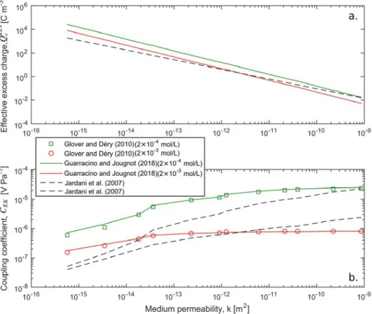
262
Figure 2: Effective excess charge density of various porous media as a function of the 263
permeability (modified from Guarracino and Jougnot, 2018). 264
265
The second approach to obtain the effective excess charge density is through an up-scaling 266
procedure. In this approach the transport of the excess charge density by the water flux in the 267
medium is explicitly considered. In order to perform this up-scaling, one must simplify the 268
problem using geometrical approximations to describe the porous medium. Following the 269
original work of von Smoluchovski (1903), it is possible to consider the electrokinetic coupling 270
phenomena occurring in a capillary (e.g., Rice and Whitehead, 1951; Packard, 1953) or in a 271
bundle of capillaries (e.g., Bernabé, 1998; Jackson, 2008, 2010; Jackson and Leinov, 2012). 272
More recently, Guarracino and Jougnot (2018) proposed an analytical mechanistic model to 273
determine the effective excess charge under saturated conditions for a bundle of capillaries. This 274
model is based on a two-steps up-scaling procedure that was proposed numerically by Jougnot et 275
al. (2012): (1) from the EDL scale to the effective excess charge in a single capillary and then (2) 276
from one capillary to a bundle of capillaries (i.e. the REV). 277
Based on the EDL description and assumptions presented in section 2.1, Guarracino and Jougnot 278
(2018) derived a closed-form equation for the effective excess charge density in a single capillary 279
with the radius R (in m), ˆR
v Q (in C m-3): 280
(
)
3 0 R A 0 w 0 0 D B B 8 ˆ ( ) 2 3 v N e C e e Q R R l k T k T ζ ζ = − − . (22) 281Then, by considering a fractal law for the pore size distribution, that is a power law distribution 282
relating the pore size R to the number of pores in the medium N(R) (e.g., Guarracino et al., 2014; 283
Tyler & Wheatcraft, 1990; Yu et al., 2003): 284 REV ( ) D R N R R = , (23) 285
where D is the fractal dimension (unitless), they derived a closed-form equation to determine the 286
effective excess charge density at the scale of the representative elementary volume (REV) (i.e., 287
the bundle of capillaries), ˆREV
v Q (in C m-3): 288 3 REV 0 0 0 A 0 w D 2 B B 1 ˆ 2 3 v e e Q N e C l k T k T k ζ ζ φ τ = − − , (24) 289
where the parameters controlling ˆREV
v
Q can be decomposed in two main parts (1) the geometrical 290
properties (i.e., petrophysical properties): porosity φ, permeability k , and hydraulic tortuosity 291
τ
and (2) the electro-chemical properties: ionic concentration, Debye length, and Zeta potential. 292Note that all these properties can be estimated independently. By arranging Eq. (24), it is possible 293
to derive the empirical relationship proposed by Jardani et al. (2007) (Eq. 21) and to obtain 294
expression for the fitting constants A1 and A2 in terms of fractal dimension and chemical
295
parameters. The performance of the model is tested with the extensive data set presented in 296
Fig. 2. 297
298
2.4.2 Under partially saturated conditions 299
Under partially saturated conditions, that is, when the water volume in the pore space diminishes, 300
the behavior of the effective excess charge is still under discussion. One could see two different 301
up-scaling approaches to determine it: (1) the volume averaging approach and (2) the flux-302
averaging approach. 303
The volume averaging approach to determine the evolution of QˆvREV(Sw) was first proposed by 304
Linde et al. (2007) to explain the data from a sand column drainage experiment and described in 305
detail by Revil et al. (2007) in a very complete electrokinetic framework in partially saturated 306
porous media. This up-scaling approach is built on the fact that no matter the medium water 307
saturation, the surface charge to counterbalance is constant. That is, when the water volume 308
decreases, the total excess charge diminishes but its density increases linearly. It yields: 309 REV,sat REV w w ˆ ˆ ( ) v v Q Q S S = . (25) 310
This approach has been successfully tested experimentally in various works mainly on sandy 311
materials (e.g., Linde et al. 2007, Mboh et al. 2012, Jougnot and Linde 2013). However, when 312
applied to more complex soils, Eq. (25) seems to fail reproducing the magnitudes observed. 313
Considering the porous medium as a bundle of capillaries provides a theoretical tool to perform 314
the up-scaling of electrokinetic properties under partial saturation. Jackson (2008, 2010) and 315
Linde (2009) propose different models to determine the evolution of the coupling coefficient with 316
varying water saturation. The distribution of capillary sizes in the considered bundle is a way to 317
take the heterogeneity of the pore space into account in the models. Building on the previous 318
works cited above, Jougnot et al. (2012) propose a new way to numerically determine the 319
evolution of the effective excess charge as a function of saturation. The numerical up-scaling 320
proposed by these authors is called flux averaging approach, by opposition to the volume 321
averaging one (Eq. 25), as it is based on the actual distribution of the water flux in the pore space 322
and therefore on the fraction of the excess charge that is effectively dragged by it. The model can 323 be expressed by: 324 Sw min Sw min R REV w ˆ ( ) ( ) ( ) ˆ ( ) ( ) ( ) R R v D R v R R D R Q R v R f R dR Q S v R f R dR =
∫
∫
, (26) 325 where ˆ ( )R vQ R is the effective excess charge density (in C m-3) in a given capillary R as expressed 326
by Eq. (21), vR( )R is the pore water velocity in the capillary (in m s-1), and fD( )R is the 327
capillary size distribution of the considered medium. Although this flux-averaging model can 328
consider any kind of capillary size distribution, Jougnot et al. (2012) propose to infer fD( )R 329
from the hydrodynamic properties of the considered porous medium. It yields two approaches: 330
(1) the water retention (WR) and (2) the relative permeability (RP) based on the corresponding 331
hydrodynamic functions. From various studies, it has been shown that the WR approach tends to 332
better predict the relative evolution of the effective excess charge density as a function of 333
saturation, while the RP approach performs better for amplitude prediction (e.g., Jougnot et al. 334
2012, 2015). Therefore, following the proposition of Jougnot et al. (2015), we suggest that the 335
effective excess charge density under partially saturated conditions can be obtained by: 336
REV REV,rel REV,sat
w w
ˆ ( ) ˆ ( )ˆ
v v v
Q S =Q S Q , (27)
337
where the saturated effective excess charge density ˆREV,sat
v
Q can be obtained from Eq. (24) and the 338
relative excess charge density REV, rel w
ˆ ( )
v
Q S can be determined using Eq. (26). 339
It is worth noting that Jougnot and Linde (2013) shown that the predictions of Eq. (25) and (26) 340
can overlap over a large range of saturation for certain sandy materials (e.g., the one used in 341
Linde et al. 2007), which explains why the volume averaging model performed well in Linde et 342
al. (2007) and possibly in Mboh et al. (2012) as they used a similar material. 343
3. Evolution of the effective excess charge 345
3.1 Evolution with the salinity 346
From the theory section, it clearly appears that the pore water salinity strongly influences the 347
electrokinetic coupling. Indeed, the pore water electrical conductivity explicitly appears in the 348
coupling coefficient definition (Eqs. 14 and 18). Nevertheless, the pore water salinity also 349
strongly affects the properties of the EDL. Eq. (3) shows its effect on the extension of the diffuse 350
layer, while many studies show that it also changes the value of the ζ-potential (e.g., Pride and 351
Morgan, 1991; Jaafar et al., 2009; Li et al., 2016). In the present approach, we use the Pride and 352 Morgan (1991) model: 353 0 0 (Cw) a blog(Cw) ζ = + , (28) 354
where a = −6.43 mV and b = 20.85 mV for silicate-based materials and for NaCl brine according 355
to Jaafar et al. (2009) if ζ is expressed in mV and 0
w
C in mol L–1. Note that the behavior of the ζ
356
-potential as a function of the salinity is challenged in the literature (e.g., see the discussion in 357
Fiorentino et al., 2016). 358
Figure 3 illustrates the evolution of the effective excess charge density as a function of the pore 359
water salinity (i.e., ionic concentration of NaCl). The experimental data come from the study of 360
Pengra et al. (1999) for different porous media, while the model is the one proposed by 361
Guarracino and Jougnot (2018) where the hydraulic tortuosity (i.e., the only parameter not 362
measured by Pengra et al., 1999) is optimized to fit the data. The overall fit is pretty good, 363
indicating that the Guarracino and Jougnot (2018) model correctly takes into account the effect of 364
the salinity on the EDL and resulting effective excess charge density. 365
367
Figure 3: Effective excess charge density of various porous media as a function of the ionic 368
concentration of the NaCl in the pore water. The experimental data have been extracted from 369
Pengra et al. (1999). 370
371
3.2 Evolution with the petrophysical properties 372
From previous section, it is clear that the effective excess charge density is dependent on 373
petrophysical properties like permeability, porosity, and hydraulic tortuosity. In contrast to other 374
models, Guarracino and Jougnot (2018) explicitly express ˆREV
v
Q as a function of these three 375
parameters. 376
Glover and Déry (2010) conducted a series of electrokinetic coupling measurements on well-377
sorted glass bead samples of different radii at two pore water salinities. They also performed an 378
extensive petrophysical characterization of each sample, providing all the necessary parameters 379
to test the model proposed by Guarracino and Jougnot (2018), except for the hydraulic tortuosity. 380
Figure 4a shows the ˆREV
v
Q predicted by this model (using
τ
= 1.2) and by the empirical 381relationship from Jardani et al. (2007) (Eq. 21). Figure 4b compares the coupling coefficient 382
measured by Glover and Déry (2010) with the coupling coefficients calculated using the QˆvREV 383
predicted by the models of Guarracino and Jougnot (2018) and Jardani et al. (2007), respectively. 384
One can see that the model informed by the measured petrophysical parameter performs better 385
and is able to reproduce the entire dataset with a single value of hydraulic tortuosity. A better fit 386
can be obtained by optimizing the hydraulic tortuosity for each sample. 387
388
Figure 4: Effective excess charge density of various porous media as a function of the 389
permeability for
τ
= 1.2. 390391
The link between effective excess charge density and hydraulic tortuosity can be explicitly seen 392
in Eq. (24). Unfortunately, the hydraulic tortuosity is not an easy parameter to measure for all 393
type of porous media; Clennell (1997) provides an extensive review of the different definitions 394
and models to estimate tortuosities in porous media. Among others, Windsauer et al. (1952) 395
proposes a simple way to relate the hydraulic tortuosity to the formation factor F, which is easier 396 to measure: 397 e F τ = φ , (29) 398
where
φ
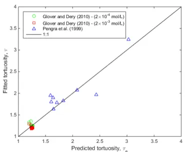
is the porosity of the medium. 399Figure 5 compares the optimized tortuosities (
τ
) to obtain the best fit of the Guarracino and 400Jougnot (2018) model for each sample showed on Figs. 3 and 4 to the predicted tortuosities (τe) 401
using Eq. (29). One can see that the best fit tortuosities fall very close to the 1:1 line showed here 402
for reference, therefore indicating that Eq. (29) provides a fair approximation for the hydraulic 403
tortuosity when it cannot be obtained otherwise. 404
405
406
Figure 5: Predicted versus best-fit tortuosities for the data from Glover and Déry (2010) and 407
Pengra et al. (1999). The plain black line corresponds to 1:1 values (i.e., τ =τe). 408
409
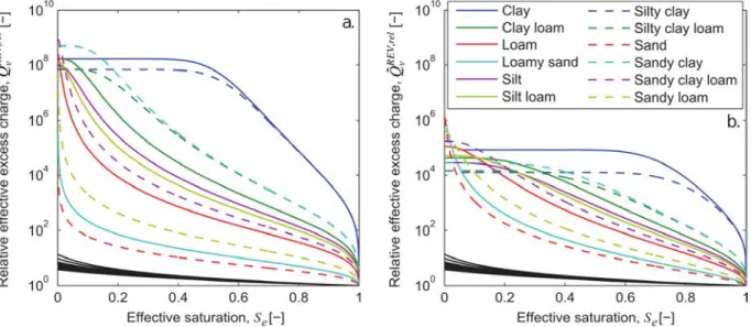
3.3 Evolution with saturation 410
The effect of the saturation on the effective excess charge density remains a vivid area of 411
investigation as explained in the theory section. In the present chapter we compare the volume 412
averaging approach of Linde et al. (2007) with the flux averaging approach of Jougnot et al. 413
(2012). Figure 6a and b show the evolution of relative excess charge densities as a function of the 414
effective saturation for the Jougnot et al. (2012) model (Eq. 26) using a pore size distribution 415
inferred from the water retention ( WR D
f ) and the relative permeability ( RP D
f ) curves, respectively. 416
The black lines correspond to the volume averaging approach for the corresponding soils. Note 417
that the x-axis represents the effective saturation, defined as: 418 1 r w w e r w S S S S − = − , (30) 419
to remove the effect of the residual water saturation r w
S differences between the soil types. It 420
explains why all the volume averaging curves are not superposed. 421
It can be noted that the effective excess charge always increases as the water saturation decreases. 422
For the volume averaging model, it is due to decreasing volume of water in the pores while the 423
amount of charges to compensate remains constant. For the flux averaging model, it is due to the 424
fact that larger pores (i.e., smaller relative volume of EDL in the capillary) are desaturating first, 425
letting the water flow through the smaller pores (i.e., smaller relative volume of EDL in the 426
capillary). Hence, the model proposed by Jougnot et al. (2012) yields a soil-specific function 427
REV
ˆ ( )
v w
Q S which strongly depends on the soil texture and shows very important changes with 428
saturation, i.e., up to 9 orders of magnitudes. 429
430
Figure 6: Effective excess charge density of various soil types as a function of the saturation 431
(modified from Jougnot et al. 2012). 432
433 434
4. Pore network determination of the effective excess charge density 435
The present section describes a numerical up-scaling procedure to determine the effective excess 436
charge density in a synthetic 2D pore network. 437
4.1 Equations of coupled fluxes in a single capillary 438
Following the formalism exposed in Bernabé (1998), the hydraulic flux Q and the electrical flux 439
J in a single capillary of radius r and length l are given by the two coupled equations: 440
(
)
( )
(
)
( )
(
)
( )
( )
(
)
2 4 0 2 0 2 0 2 0 2 2 2 0 0 0 2 1 8 2 1 2 2 cosh r u d u d r u d r r u d f P P r V V r Q r r dr l r l P P r J r r dr r l d r ze r V V r dr r dr dr kT l πεε ζ π ψ η η ζ πεε ψ η ζ ψ ψ πε ε πσ η − − = − + − − = − − − + ∫
∫
∫
∫
(31) 441where Pu (resp. Vu) is the upstream hydraulic pressure (resp. the electrical potential) and Pd (resp.
442
Vd) the downstream pressure (resp. potential). The computation of the local electrical potential
443
distribution ψ inside the capillary is obtained by solving the Poisson-Boltzmann equation inside 444
infinite cylinders, as done by Leroy and Maineult (2018). 445
The set of Eqs. (31) can be written as: 446
(
)
(
)
(
)
(
)
h c u d u d c e u d u d Ql P P V V Jl P P V V γ γ γ γ = − − + − = − − − (32) 447 where γhis the modified hydraulic conductance (in m4 Pa-1 s-1), γe
the electrical conductance (in 448
S m), and γc the coupling conductance (in m4 V-1 s-1). 449
450
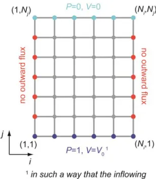
4.2 2D tube network and linear system for the pressure and the electrical potential 451
We consider a square random tube network as depicted in Fig. 7, for which all tubes are of length 452
l (in m). 453
455
Figure 7: Tube network and boundary conditions. 456
457
Writing the conservation laws (Kirchhoff’s laws, 1845) for the hydraulic flux and the electrical 458
flux at each node of the network, combined with the appropriate boundary conditions, provides a 459
linear system to be solved, whose unknown are the hydraulic pressures and electrical potential Pi,j
460
and Vi,j at all nodes and the electrical potential V0 (for more details, see Appendix A).
461 462
4.3 Computation of the petrophysical parameters 463
The electrokinetic coupling coefficient (in V Pa-1) is computed using: 464 0 0 0 0 1 EK V V C V P − ∆ = = = ∆ − . (33) 465
The excess of charge density is given by reorganizing Eq. (18): 466 ˆ EK v C Q k ησ = − , (34) 467
Neglecting the surface conductivity and introducing the formation factor gives: 468 ˆ w EK v C Q kF ησ = − . (35) 469
For the computation of the quantities k
φ
−1and F
φ
, see Appendix B. 470471
4.4 Applications 472
We ran computations on uncorrelated random networks (i.e., the distribution of the tube radii is 473
totally uncorrelated) of size 100 by 100 nodes (19800 tubes). We used a distribution such that the 474
decimal logarithm of the radius is normally distributed, as done by Maineult et al. (2017) – see 475
Fig. 8. The probability P that log(r) is less than X is given by: 476
( )
(
log)
1 1erf log(
)
2 2 SD 2 peak X r P r X − ≤ = + (36) 477
where SD is the standard deviation. We explored different values of rpeak (i.e., 0.1, 0.2, 0.3, 0.5, 1,
478
2, 3, 5 and 10 µm), and took SD=0.5. 479
480
Figure 8: Example of random uncorrelated media. Experimental distribution (a) of the tube radii 482
(the decimal logarithm of the pore tube radius distribution is normally distributed, with a mean 483
radius of 10 µm and a standard deviation of 0.5) associated with the network (100 ×100 nodes, 484
19800 tubes) shown in b (modified from Maineult et al., 2017). 485
486
Note that to compute the fluid conductivity σw associated with the concentration Cw0, we used the
487
empirical relation given by Sen and Goode (1992) for NaCl brine: 488
(
4 2)
2.36 0.099 32 5.6 0.27 1.510 1 0.214 w T T T M M M σ = + − − − + + (37) 489where T is the normal (i.e., not absolute) temperature (in °C) and M is the molality (in mol kg–1). 490
To convert the concentration 0
w
C into molality, we use the CRC Handbook Table at 20°C (Lide 491
2008). The ζ-potential is then obtained from the relation given by Jaafar et al (2009) (Eq. 28). 492
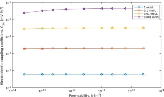
Figure 9 shows the electrokinetic coupling coefficients calculated for different 2D pore networks 493
having different permeabilities. For ionic concentrations larger than 0.01 mol/L, the coupling 494
coefficient appears not to be dependent on the permeability despite the influence of the 495
permeability in its definition (Eq. 18). This is a result of the linearly dependence on the 496
permeability of the effective excess charge density, canceling the permeability in Eq. (18). That 497
can be clearly seen in Fig. 10, where the analytical model of Guarracino and Jougnot (2018) 498
predicts accurately the evolution of the effective excess charge density for the synthetic 2D pore 499
network. Note that this very good fit is obtained from all the calculated parameters, with only one 500
unknown, which has been fitted:
τ
= 2.3. 501Then, for 0.001 mol/L, the coupling coefficient tends to decrease for the lowest permeabilities 502
(below 10-12 m2), i.e., the smallest pore sizes, which also correspond to the poorer fit of Eq. (24) 503
on the synthetic data. This can be expected from the assumptions of the Guarracino and Jougnot 504
(2018) model which is only valid when the EDL thickness is small enough in comparison to the 505
pore size. Low permeabilities and low salinities therefore show a limitation of their model, as the 506
local potential distribution in the EDL must be computed by solving the Poisson-Boltzmann 507
equation (see Leroy and Maineult, 2018). 508
510
Figure 9: Coupling coefficient of the 2D pore networks as a function of permeability for different 511
NaCl concentrations. 512
513
514
Figure 10: Evolution of the excess charge density as a function of permeability for different NaCl 515
concentrations: comparison between the 2D pore network results and model predictions of 516
Guarracino and Jougnot (2018) for the corresponding ionic concentrations and
τ
= 2.3. 5175. Use of the effective excess charge in numerical simulations 519
The present section illustrates the usefulness of the effective excess charge approach to model the 520
streaming potential distribution in two kinds of complex media: a partially saturated soil and a 521
fractured aquifer. 522
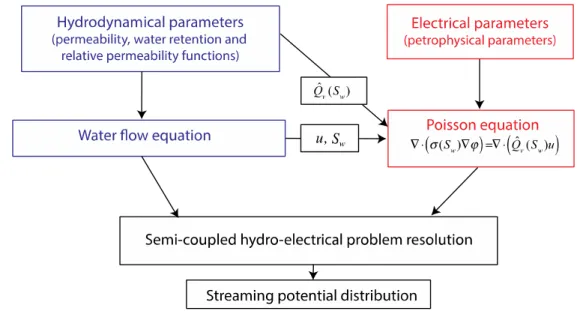
5.1 Rainwater infiltration monitoring 523
Figure 11 describes the numerical framework that we use to simulate the streaming potential 524
distribution resulting from a rainfall infiltration in a sandy loam soil. As explained in the theory 525
section, the results of the hydrological simulation are used as input parameters for the electrical 526
problem. In that scheme, it is clear that the electrokinetic coupling parameter is the effective 527
excess charge density even if the water saturation distribution also plays a role through the 528
electrical conductivity, affecting the amplitude of the SP signals. 529
530
531
Figure 11: Numerical framework for the simulation of the streaming potential distribution in a 532
partially saturated porous medium. 533
534
We consider a homogeneous sandy loam soil subjected to a rainfall event (Fig. 12a). The initial 535
hydraulic conditions of the soil are set to hydrostatic equilibrium with a water table localized at 536
2.5 m depth. Following the work of Jougnot et al. (2015), the hydrological problem is solved 537
using Hydrus 1D. This code solves the Richards equation to determine the evolution of the water 538
saturation (Fig. 12b) and Darcy velocity as a function of depth and time. We choose the van 539
Genuchten model to describe the water retention and the relative permeability functions, using 540
the average hydrodynamic properties for a sandy loam soil proposed by Carsel and Parrish 541
(1988). 542
The electrical problem is solved using a home-made code (for details please refer to Jougnot et 543
al., 2015). As illustrated in Fig. 11, the hydrological simulation ouputs (i.e., the water saturation 544
and the Darcy velocity distribution in both space and time) are used as input parameters for the 545
electrical problem. The electrical conductivity is determined using Archie (1942) with the 546
following petrophysical parameters: m = 1.40 the cementation exponent and n = 1.57 the 547
saturation exponent. The effective excess charge is determined using Eq. (27) in which 548
REV,rel
ˆ ( )
v w
Q S can be obtain from the WR or the RP flux averaging approach of Jougnot et al. 2012, 549
or using the volume averaging approach of Linde et al. (2007) as explained in Section 2.4.2 (Fig. 550
13a). 551
Figure 12c shows the results of the numerical simulation of the streaming potential for virtual 552
electrodes localized at different depths in the soil. Note that the reference electrode is localized at 553
a depth of 3˚m. As the rainwater infiltration front progresses in the soil, the SP signals starts to 554
increase. An electrode localized at the soil surface should be able to capture the highest signal 555
amplitude during the rainfall, while the deeper electrodes show a time shift related to the time 556
needed for the water flow to reach the electrode. The signal amplitude also decreases with depth 557
as the Darcy velocity diminishes during the infiltration. The multimodal nature of the rainfall also 558
vanishes, showing only a single SP peak at a depth of 5 cm. The Q Sˆ ( )v w function used to plot 559
Fig. 12c is the RP approach from Jougnot et al. (2012). Figure 13b shows the strong influence of 560
the chosen approach on the vertical distribution of the signal amplitude at two different times 561
(t = 2 and 10 d). These results are consistent with the findings of Linde et al. (2011), that is, the 562
volume averaging model of Linde et al. (2007) does not allow to reproduce the large vertical SP 563
signals that can be found in the literature (e.g., Doussan et al., 2002; Jougnot et al., 2015). 564
565
Figure 12: Simulation results of the rainwater infiltration: (a) precipitation, (b) water saturation, 566
and (c) streaming potential as a function of time. 567
569
Figure 13: (a) Comparison of the effective excess charge density as a function of the water 570
saturation using Jougnot et al. (2012) RP and WR approaches and Linde et al. (2007). (b) 571
Vertical distribution of the SP signal resulting for the rainwater infiltration using the 572
corresponding ˆQ Sv( w) function at two different times, t =2 and 10 d, for the plain and the 573
dashed lines, respectively. 574
575
5.2 Pumping in a fractured medium 576
The effective excess charge can also be used for modeling the streaming potential arising from 577
groundwater flow in fractured media (e.g., Fagerlund and Heinson, 2003; Wishart et al., 2006; 578
2008; Maineult et al., 2013). Existing studies focusing on this phenomenon in fractured rocks 579
suggest that monitoring the corresponding streaming potential under pumping conditions can help 580
to identify the presence of fractures that interact with the surrounding matrix (Roubinet et al., 581
2016; DesRoches et al, 2017). This has been demonstrated with numerical approaches relying on 582
a discrete representation of the considered fractures that are coupled to the matrix by using either 583
the finite element method with adapted meshing (DesRoches et al, 2017) or the finite volume 584
method within a dual-porosity framework (Roubinet et al., 2016). 585
The latter method is used here to illustrate the sensitivity of SP signals to hydraulically active 586
fractures, and in particular to fractures having important fracture-matrix exchanges. For this 587
purpose, we consider the coupled fluid flow and streaming potential problem described in 588
Figure 11 that we apply to fractured porous domains under saturated conditions. In this case, the 589
fluid flow problem is solved by considering Darcy’s law and Darcy-scale mass conservation 590
under steady-state conditions, and the effective excess charge is evaluated from the fracture and 591
matrix permeability by adapting the strategy proposed in Jougnot et al. (2012) to two infinite 592
plates having known separation and using the empirical relationship defined by Jardani et al. 593
(2007), respectively. As shown in Roubinet et al. (2016), both fluid flow and streaming current 594
must be simulated in the fractures and matrix to adequately solve this problem, even if the matrix 595
is characterized by a very low permeability. Furthermore, relatively small fracture densities 596
should be considered in order to individually detect the fractures that are hydraulically active. 597
Figure 14a, b, and c show three examples of fractal fracture network models defined by 598
Watanabe and Takahashi (1995) for characterizing geothermal reservoirs and used in Gisladottir 599
et al. (2016) for simulating heat transfer in these reservoirs. In these models, the number of 600
fractures and the relative fracture lengths (i.e., the ratio of fracture to domain length) are defined 601
from the fracture density, the smallest fracture length, and the fractal dimension that are set to 602
2.5, 0.1, and 1 m, respectively, considering a square domain of length = 100 m. The positions 603
of these fractures are randomly distributed, their angle can be equal to = 25° or = 145° 604
with equal probability, and their aperture is set to 10-3 m. Note that we also add a deterministic 605
fracture whose center is located at the domain center and whose angle is set to (represented in 606
red in Figs. 14a-c). Finally, the fracture and matrix conductivity are set to 5 × 10 and 5 × 10 607
S m-1, respectively, and the matrix permeability to 10 m2. 608
The fluid flow and streaming potential problem is solved by considering (i) a pumping rate of 609
10 m3 s-1 applied at the domain center, (ii) gradient head boundary conditions with hydraulic 610
head set to 1 and 0 m on the left and right sides of the domain, respectively, and (iii) a current 611
insulation condition on all borders. Figure 1 shows the resulting difference of potential ∆ , and 612
∆ where the white (Figs. 14d-f) and black (in Figs. 14g-i) dots represent the two largest SP 613
signals measured along the dashed white circles that are plotted in Figs. 14d-f. These results show 614
that a strong SP signal is observed for the primary fracture in which the pumping rate is applied 615
when this fracture is not intersected by secondary fractures that are close to the pumping well 616
(Figs. 14d and g). On the contrary, when the primary fracture is intersected by secondary 617
fractures that are close to the pumping well and not connected to the domain borders, strong SP 618
signals are observed at the extremities of the single secondary fracture (Figs. 14e and h) or the 619
pair of secondary fractures (Figs. 14f and i). As demonstrated in existing studies (DesRoches et 620
al, 2017; Roubinet et al., 2016), these results suggest that strong SP signals are associated with 621
hydraulically active fractures, and that the largest values of SP measurements are related to 622
important fracture-matrix exchanges. 623
(a) (b) (c) (d) (e) (f) (g) (h) (i) 625
Figure 14 – (a-c) Studied fractured domains where the red cross represents the position of the considered pumping well. (d-f) Spatial distribution of
626
the SP signal ∆ , (in mV) with respect to a reference electrode located at position (x,y)=(0,0). (g-i) Polar plots of the SP signal ∆ (in mV)
627
along the dashed white circle plotted in (d-f) with respect to the minimum value measured along this circle and represented with a white cross.
628 0 50 100 0 50 100 0 50 100 0 50 100 0 50 100 0 50 100 0 50 100 0 50 100 0 20 40 60 80 100 0 50 100 0 50 100 0 20 40 60 80 100 0 50 100 0 50 100 0 20 40 60 80 100
6. Discussion and conclusion 629
Modeling of the streaming current generation and the corresponding electrical field requires a 630
good understanding of electrokinetic coupling phenomena that occur when the water flows in 631
porous and fractured media. This modeling can be done with two electrokinetic coupling 632
parameters: coupling coefficient and effective excess charge. In this chapter we focused on the 633
latter. 634
Considering the effective excess charge approach is quite recent (Kormiltsev et al. 1998) 635
compare to the use of the coupling coefficient. Unlike the coupling coefficient, the effective 636
excess charge density shows a strong dependence on petrophysical parameters (permeability, 637
porosity, ionic concentration in the pore water). This has been highlighted by both empirical 638
(Titov et al. 2001; Jardani et al. 2007) and mechanistic (Jougnot et al., 2012; Guarracino and 639
Jougnot, 2018) approaches. The mechanistic approaches that we discuss in this chapter are based 640
on the up-scaling process called flux-averaging as they propose an effective value for the excess 641
charge density which is related to pore scale properties of the EDL and how the water flows 642
through it. 643
Under saturated conditions, Guarracino and Jougnot (2018) model shows a linear dependence 644
with geometrical properties (permeability, porosity, hydraulic tortuosity) and non-linears ones to 645
chemical properties (ionic concentration, zeta potential). In section 3 and 4, we show that is 646
provides good match with published laboratory data for various types of media as long as the 647
model assumptions are respected (i.e., the pore radius should 5 times larger than the Debye 648
length). The numerical simulations of 2D synthetic porous networks following the approaches of 649
Bernabé (1998) and Maineult et al. (2017) strongly confirm these dependences. 650
Under partially saturated conditions, Jougnot et al. (2012) model shows a strong dependence of 651
the effective excess charge density on the medium hydrodynamic properties of the porous 652
medium. The function ˆ (Q Sv w) becomes medium dependent and generally increases when the 653
saturation decreases (up to 9 orders of magnitude). 654
The effective excess charge density approach has proven to be fairly useful to model the SP 655
signal generation in complex media. In this chapter, we illustrate that with two examples: the SP 656
monitoring of a rainfall infiltration and the SP response to pumping water in a fractured aquifer. 657
In both cases the use of the effective excess charge as electrokinetic coupling parameter makes it 658
simple to directly relate the streaming current generation to the water flux distribution in the 659
medium and to explicitly take into account the medium heterogeneities below the REV scale (due 660
to, for instance, saturation distribution, fractures). We believe that the development of that 661
approach will help developing the use and modeling of streaming potentials in all kinds of media. 662
Appendix A: Equations for the pressure and electrical potential 664
This appendix details the calculation of the pressure and the electrical potential in the pore 665
network. The Kirchhoff (1845) laws for the water flow and the electrical current at node of 666
coordinates (i,j), which express the conservation of mass and the conservation of charge 667 respectively, write: 668
(
)
(
)
(
)
(
)
(
)
(
)
(
)
(
)
1, , , 1, 1, , , 1, 1, , , 1, 1, , , 1, , 1 , , , 1 , 1 , , , 1 , 1 , , , 1 , 1 , , , 1 1, , , 0 h c i j i j i j i j i j i j i j i j h c i j i j i j i j i j i j i j i j h c i j i j i j i j i j i j i j i j h c i j i j i j i j i j i j i j i j c i j i j i P P V V P P V V P P V V P P V V P γ γ γ γ γ γ γ γ γ − → − − → − + → + + → + − → − − → − + → + + → + − → − − + − − − + − − − + − − − + − =(
)
(
)
(
)
(
)
(
)
(
)
(
)
(
)
1, 1, , , 1, 1, , , 1, 1, , , 1, , 1 , , , 1 , 1 , , , 1 , 1 , , , 1 , 1 , , , 1 0 e j i j i j i j i j i j c e i j i j i j i j i j i j i j i j c e i j i j i j i j i j i j i j i j c e i j i j i j i j i j i j i j i j P V V P P V V P P V V P P V V γ γ γ γ γ γ γ − − → − + → + + → + − → − − → − + → + + → + − − − + − − − + − − − + − − − = , (A1) 669for the node located in the interior of the network. 670
Inside the domain (i.e., for the indexes (i,j) ∈ [2,Ni–1]×[2,Nj–1]), equations (A1) can be
671 rewritten ; 672 1, , 1, 1, , 1, , , , 1 , , 1 , 1 , , 1 1, , 1, 1, , 1, , , , 1 , , 1 , 1 , , 1 1, , 1, 1, , 1, 0 h h h h h i j i j i j i j i j i j i j i j i j i j i j i j i j i j c c c c c i j i j i j i j i j i j i j i j i j i j i j i j i j i j c c i j i j i j i j i j i P P P P P V V V V V P P γ γ κ γ γ γ γ κ γ γ γ γ − → − + → + − → − + → + − → − + → + − → − + → + − → − + → + + − + + − − + − − = − − , , , 1 , , 1 , 1 , , 1 1, , 1, 1, , 1, , , , 1 , , 1 , 1 , , 1 0 c c c j i j i j i j i j i j i j i j i j e e e e e i j i j i j i j i j i j i j i j i j i j i j i j i j i j P P P V V V V V κ γ γ γ γ κ γ γ − → − + → + − → − + → + − → − + → + + − − + + − + + = , (A2) 673 with: 674
(
)
(
)
(
)
, 1, , 1, , , 1 , , 1 , , 1, , 1, , , 1 , , 1 , , 1, , 1, , , 1 , , 1 , h h h h h i j i j i j i j i j i j i j i j i j c c c c c i j i j i j i j i j i j i j i j i j e e e e e i j i j i j i j i j i j i j i j i j κ γ γ γ γ κ γ γ γ γ κ γ γ γ γ − → + → − → + → − → + → − → + → − → + → − → + → = + + + = + + + = + + + , (A3) 675In i=1 (no outward flux), j∈[2,Nj–1], we have (see Figure 1):