Analysis of an optimal hidden Markov model for secondary structure prediction

HAL Id: hal-02666900

https://hal.inrae.fr/hal-02666900

Submitted on 31 May 2020

HAL is a multi-disciplinary open access

archive for the deposit and dissemination of

sci-entific research documents, whether they are

pub-lished or not. The documents may come from

teaching and research institutions in France or

abroad, or from public or private research centers.

L’archive ouverte pluridisciplinaire HAL, est

destinée au dépôt et à la diffusion de documents

scientifiques de niveau recherche, publiés ou non,

émanant des établissements d’enseignement et de

recherche français ou étrangers, des laboratoires

publics ou privés.

Juliette Martin, Jean-François Gibrat, Francois Rodolphe

To cite this version:

Juliette Martin, Jean-François Gibrat, Francois Rodolphe. Analysis of an optimal hidden Markov

model for secondary structure prediction. BMC Structural Biology, BioMed Central, 2006, 6 (25),

pp.1-20. �10.1186/1472-6807-6-25�. �hal-02666900�

Open Access

Research article

Analysis of an optimal hidden Markov model for secondary

structure prediction

Juliette Martin*

_{, Jean-François Gibrat}

_{and François Rodolphe}

Address: 1_{INSERM U726, Equipe de Bioinformatique Génomique et Moléculaire Université Denis Diderot Paris 7, 2 place jussieu, 75251 Paris} Cedex 05, France and 2_{INRA, Unité Mathématiques Informatique et Génome, Domaine de Vilvert, 78352 Jouy en Josas Cedex, France} Email: Juliette Martin* - juliette.martin@jouy.inra.fr; Jean-François Gibrat - jean-francois.gibrat@jouy.inra.fr;

François Rodolphe - francois.rodolphe@jouy.inra.fr * Corresponding author

Abstract

Background: Secondary structure prediction is a useful first step toward 3D structure prediction. A number of successful secondary structure prediction methods use neural networks, but unfortunately, neural networks are not intuitively interpretable. On the contrary, hidden Markov models are graphical interpretable models. Moreover, they have been successfully used in many bioinformatic applications. Because they offer a strong statistical background and allow model interpretation, we propose a method based on hidden Markov models.

Results: Our HMM is designed without prior knowledge. It is chosen within a collection of models of increasing size, using statistical and accuracy criteria. The resulting model has 36 hidden states: 15 that model α-helices, 12 that model coil and 9 that model β-strands. Connections between hidden states and state emission probabilities reflect the organization of protein structures into secondary structure segments. We start by analyzing the model features and see how it offers a new vision of local structures. We then use it for secondary structure prediction. Our model appears to be very efficient on single sequences, with a Q3 score of 68.8%, more than one point above PSIPRED prediction on single sequences. A straightforward extension of the method allows the use of multiple sequence alignments, rising the Q3 score to 75.5%.

Conclusion: The hidden Markov model presented here achieves valuable prediction results using only a limited number of parameters. It provides an interpretable framework for protein secondary structure architecture. Furthermore, it can be used as a tool for generating protein sequences with a given secondary structure content.

Background

Predicting the secondary structure of a protein is often a first step toward 3D structure prediction of a particular protein. In comparative modeling, secondary structure prediction is used to refine sequence alignments, or to improve the detection of distant homologs [1]. Moreover, it is of prime importance when prediction is made

with-out a template [2]. For all these reasons protein secondary structure prediction has remained an active field for years. Virtually all statistical and learning methods have been applied to this task. Nowadays, the best methods achieve prediction rate of about 80% using homologous sequence information. A survey of the Eva on-line evaluation [3] shows that the top performing methods include several

Published: 13 December 2006

BMC Structural Biology 2006, 6:25 doi:10.1186/1472-6807-6-25

Received: 25 August 2006 Accepted: 13 December 2006 This article is available from: http://www.biomedcentral.com/1472-6807/6/25

© 2006 Martin et al; licensee BioMed Central Ltd.

This is an Open Access article distributed under the terms of the Creative Commons Attribution License (http://creativecommons.org/licenses/by/2.0), which permits unrestricted use, distribution, and reproduction in any medium, provided the original work is properly cited.

approaches based on neural networks, e.g. PSIPRED by Jones et al [4], PROFsec and PHDpsi by Rost et al [5]. Recently several publications reported secondary structure prediction using SVM [6-8]. A number of attempts using Hidden Markov Models (HMM) have also been reported. A particularity of these models is their ability to allow an explicit modeling of the data. The first attempt to predict secondary structure with HMMs was due to Asai et al [9]. Asai et al presented four sub-models, trained separately on pre-clustered sequences belonging to particular local structures: alpha, beta, coil and turns. The sub-models, each of them made of four or five hidden states, were then merged into a single model, achieving a Q₃ score of 54.7%. At the same period, Stultz et al [10,11] proposed a collection of HMMs representing specific classes of pro-teins. The models were "constructed as generalization of the study-set example structures in terms of allowed con-nectivities and surface loop/turn sizes" [10]. This involved the distinction of N-cap and C-cap positions in helices, an explicit model of amphipatic helices and β-turns. Each model being specific of a protein class, the method required first that the appropriate hidden Markov model be selected and then used to perform the secondary struc-ture prediction. The Q₃ scores, reported for only two pro-teins, were respectively 66 and 77%. Goldman et al [12-15] proposed an approach unifying secondary structure prediction and phylogenetic analysis. Starting with an aligned sequence family, the model was used to predict the topology of the phylogenetic tree and the secondary structure. The main feature of this model was the inclu-sion of the solvent accessibility status, and the constrained transitions to take into account the specific length distri-bution of secondary structure segments. The Q₃ score, reported for only one sequence family, was 65.7% using single sequence and 74.4% using close homologs. Later, Bystroff et al [16] proposed a complex methodology based on the I-Sites fragment library. One of the models was dedicated to the prediction of secondary structures. The model construction made use of a number of heuris-tic criteria to add or delete hidden states. The resulting models were quite complex and modeled the protein 3D structures in term of succession of I-site motifs. The pre-diction accuracy of the model dedicated to secondary structure prediction was 74.3%, using homologous sequence information. Other approaches used slightly dif-ferent type of HMM, based on the concept of a sliding window along the secondary structure sequence. Crooks and Brenner [17] proposed a methodology where a hid-den state represents a sliding window along the sequence. The prediction accuracy was 66.4% for single sequences and 72.2% with homologous sequence information. Zheng et al [18] used a similar approach in combination with amino-acid grouping, achieving a Q₃ score of 67.9% on single sequences. An extension of hidden Markov Model, semi-HMM, were also applied to secondary

struc-ture prediction by several groups [19-21]. These models allow an explicit consideration of the length of secondary structures. Very recently, Aydin et al claimed a Q₃ score of 70.3% for single sequences [22]. Chu et al [21] obtained a Q₃ score of 72.8% using homogous sequence informa-tion.

Here, we exploit a novel HMM learned from secondary structures without taking into account prior biological knowledge [23]. Because the choice of a particular model does not rely on any prior constraints, the HMM itself is an interesting tool to reveal hidden features of the internal architecture of secondary structures. We first analyze in detail the model. We then evaluate its predictive potential on single sequences and on multiple sequence informa-tion using an evaluainforma-tion data set of 506 sequences and a data set of 212 sequences obtained from the EVA Web site [24]. The influence of the secondary structure assignment method on the performance is also discussed. The predic-tion results appear very promising and open the perspec-tive for further refinements of the method.

Results and discussion

Hidden Markov model selection

The optimal hidden Markov model for secondary struc-ture prediction, referred as OSS-HMM (Optimal Second-ary Structure prediction Hidden Markov Model), was chosen using three criteria: the Q₃ achieved in prediction, the Bayesian Information Criterion (BIC) value of the model and the statistical distance between models. The whole selection procedure described in details in [23]. Here we only present the main steps of the selection. Let n_H, n_b and n_c be the number of hidden states that model respectively α-helices, β-strands and coils. The optimal model selection was done in three steps. In the first step, we set n_H = n_b = n_c = n and models were estimated with n varying from 1 to 75. The Q₃ score evolution indicated that 10 to 15 states were sufficient to obtain good predic-tion level without over-fitting and that increasing n above 15 had little impact on the prediction. The BIC selected a model with n = 14. The statistical distances between mod-els revealed a great similarity across modmod-els for n varying from 13 to 17. In the second step, models were thus esti-mated with (1) nH = 1 to 20 and nb = nc = 1, (2) nb = 1 to 15 and n_H = n_c = 1 or (3) n_c = 1 to 15 and n_H = n_b = 1. The BIC selected (1) n_H = 15, (2) n_b = 8 and (3) n_c = 9. In the third step, all the architectures were tested with nH varying from 12 to 16, n_b from 6 to 10 and n_c from 3 to 13. The BIC selected the optimal model having n_H = 15, n_b = 9 and n_c = 12, i. e., a total of 36 hidden states. Overall, nearly 300 dif-ferent model architectures were tested in this procedure [23]. The automatic generation of a HMM topology has been previously addressed by several groups [25-29]. Two main strategies were used: the first one consists in build-ing models of increasbuild-ing size startbuild-ing from small models

[25,29] and the second one, inversely, consists in progres-sively reducing large models [26,28]. Regarding the first strategy, the use of genetic algorithm was introduced and applied to the modeling of DNA sequences [25,29]. In the approach presented by Won et al [29], an initial popula-tion of hidden Markov models with 2 states is submitted to an iterative procedure of mutations, training and selec-tion. There are five types of mutation: addition or deletion of one hidden state, addition or deletion of one transition and cross-over, consisting in exchanging several states between two HMMs. The second strategy requires the use of a pruning algorithm and was applied to language processing [26] and to describe the structure of body motion data [28]. The initial model, consists of an explicit modeling of the training data: each sample is represented by dedicated HMM states. Hidden states are then removed iteratively by merging two states. The merging criterion is based on the evolution of the log-likelihood.

Our approach of automated selection of HMM topology is related to the first strategy because we also start from small models and increase them afterward. However, Won et al note that their mutation operations, even if they do allow highly connected models, bias the architectures toward chain structures [29]. A previous experience of knowledge-based design of HMM for secondary structure prediction [30] convinced us that highly connected mod-els are more appropriate in our case. We adopt a system-atic approach, when we introduce a new state all transitions between hidden states are initially allowed. We then let the system evolve. Our final model does not exhibit a chain structure. A major concern of the genetic algorithm applied to HMM topology seems to be the over-fitting of the model toward learning data [25,29]. In our approach, the over-fitting is monitored by considering an independent set of structures that is never used in the cross-validation procedure. An original aspect of our method is that we not only check the fit with the model but also the predictive capabilities on these independent data. The other strategy described in the literature based on the merging of states requires the manipulation of large initial models. The large size of the learning datasets available for secondary structure prediction might be a problem when employing such a strategy. Nonetheless, a common feature of our approach with the work of Vasko et al [28] is the use of initial models were all transitions are allowed.

It is likely that the appropriate strategy for automated topology selection depends on the amount and nature of data to be modeled. Here we are confronted with a prob-lem with large datasets and, presumably, a complex con-nected underlying structure. Our approach results in a model having a reasonable number of parameters

although it is larger and more complex than the one we designed in a knowledge-based approach [30].

Hidden Markov model analysis

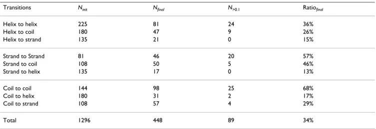
Our optimal model OSS-HMM was built without prior knowledge and without imposing any constraint. Thus, it is interesting to examine the final model as it reveals the internal architecture of secondary structures learned by the model. In the following section, we will describe the main features of the model obtained with DSSP assign-ment and link these observations with previous studies. All transitions between hidden states are initially allowed. As shown in Table 1, many transitions in the final model are estimated to have probability zero. Only 36% of potential transitions remain within the helix box, 57% within the strand box and 68% in the coil box. This high-lights a first feature of secondary structures: even though helices require 15 hidden states they can be modeled by relatively few transitions. On the contrary, β-strand sequences are fuzzier, with a higher connectivity between hidden states. Thus, the paths within the helix box are more constrained than in the strand box. The final model has 448 non-null transitions (out of 1296), of which 89 have a probability greater than 0.1, for a total of 1096 free parameters.

The structure of OSS-HMM is presented in Figure 1. For the sake of clarity, only transitions with probabilities larger than 0.1 are shown. Hidden states are colored according to their amino acid preference. The blue figure close to each state is its Neq value. The Neq value of a hid-den state is an estimation of the number of output states, derived from the Shannon Entropy:

where p(s; r) denotes the transition probability from state s to state r. The sum is taken over all the hidden states. Neq varies from 1 (only one output state) to the total number of hidden states (a state uniformly connected to all the others, including itself). Emission parameters are also pre-sented in the lower part of Figure 1. The emission proba-bility of each amino-acid in each hidden state is given using preference score relative to amino-acid background frequencies.

Some general remarks can be made from this representa-tion:

• The different secondary structures are characterized by different transition usage. Very strong transitions appear in the helix box, whereas they are weaker in strand and

Neq s p s r p s r

r

coil boxes. This is confirmed for helices since some helical states have very low Neq: e. g., H3, H2, H9 and H1 have Neq lower than 2, meaning that the number of output states is limited. No such states are apparent in the strand and coil boxes. The mean Neq value per state is 3.28 for helix, 4.70 for strand and 5.44 for coil. This confirms the observations made from Table 1: helices appear very "structured" motifs with strong transitions and few paths allowed, whereas strands appear to be "fuzzier", less con-strained, with many alternative paths and relatively low transitions probabilities. The coil box is even less struc-tured than the strand box.

• An examination of amino acid preference scores shows that hidden states specifically tend to avoid particular res-idues (many scores less than -2), rather than favor other ones (few scores greater than 2). This seems to denote a kind of "negative design", where there is a stronger con-straint not to include particular residues, than to have some others.

Helix architecture

Helices in proteins are characterized by the so-called amphipathic rule (also known as helical wheel rule): one face is in contact with the solvent and thus bears hydrophilic residues and one face is in contact with the protein interior and shows preference for hydrophobic residues. The canonical a helix has a periodicity of 3.6. The helix periodicity and the amphipathic rule generate a periodicity of 3 or 4 in terms of amino acid properties in the sequence.

The helix box is characterized by a topology that allows unidirectional paths through the graph.

• There is only one entry state for helices: state H3. The amino acid preference of this state is peculiar since it does not favor nor disfavor any amino acids except for a slight tendency to prefer proline and to avoid asparagine. Only state c10 shows a similar lack of strong preference for amino acids (i.e., without score larger than 2 or smaller than -2 and only two scores greater than 1 or less than -1). • Two alternative trajectories among the states are then possible: a "bypass" trajectory proceeding to state H7 and exiting the helix at state H6 and the "main" trajectory that is detailed below. Note that there is a small probability to get back to the main trajectory from the bypass trajectory (state H7). Interestingly this state, H7, is the only helix state with a self transition.

• States belonging to the main trajectory can be divided into two groups: core states (H10, H14, H2, H9, H1, H8, H12) and exit states (H4, H15, H11, H5, H13). As expected from the helix periodicity and amphipathic rule, the graph shows a mixture of 3-state and 4-state cycles with characteristic patterns of hydrophobic and hydrophilic preferences. It is likely that the strong direc-tionality observed between the core states is due to the fact that once in a helix the system must remain in this helix for at least 4 or 6 residues, i.e., one turn or one turn and a half. In other words, the core states correspond to the beginning of a helix.

• The second group of states, the exit states, shows the same 3-state and 4-state cycles with similar patterns of hydrophilic or hydrophobic preferences as the core states but now the cycles can be interrupted at any time to move Table 1: Number of transitions in the final 36 states HMM

Transitions N_init N_final N_>0.1 Ratio_final

Helix to helix 225 81 24 36% Helix to coil 180 47 9 26% Helix to strand 135 21 0 15% Strand to Strand 81 46 20 57% Strand to coil 108 50 5 46% Strand to helix 135 17 0 13% Coil to coil 144 98 25 68% Coil to helix 180 31 2 17% Coil to strand 108 57 4 29% Total 1296 448 89 34%

N_init: number of allowed transitions in the initial model, N_final: number of non-null transitions in the final model, N_>0.1: number of transitions associated with probabilities greater than 0.1 in the final model, Ratio_final: percentage of non-null transitions relative to the initial number.

to a coil state. This shows that helices can end without the need for completing a turn.

Strand architecture

The strand box shows a different structure. The progres-sion through the graph is also rather directional:

• There are 3 entry states (b3, b5, b7) that are all intercon-nected. All entry states are also connected to the same state, b1, that belongs to the core of the strand architec-ture.

Final 36 hidden states HMM learned using DSSP assignment

Figure 1

Final 36 hidden states HMM learned using DSSP assignment. Upper part: hidden state graph. Only transitions associ-ated with probabilities greater than 0.1 are shown. The larger the transition probabilities the thicker the arrows. States are colored according to their amino acid preference (hydrophobic versus hydrophilic). Purple state indicates no strong amino acid preference and red states strongly favor glycine. The two groups of coil states (c1, c6, c12, c5, c4) in green and (c3, c2, c8, c10, c9) in red are discussed in the text. For periodic secondary structures, helix and strand, the entry and exit states are indicated by different symbols. Lower part: amino-acid propensities of each hidden state. Propensities are measured by log-odd scores. The propensity score of amino-acid a for state s is given by: , with P(a | s) the emission probability of amino-acid a in state s and f(a) the background frequency of a in the dataset. A score equal to 1 means that the amino-amino-acid is twice as frequent in state s as in the whole dataset.

p=>0.75 hydrophilic preference hydrophobic preference Helix 3 10 14 2 9 1 8 12 4 15 11 5 13 7 6 C F L I V W Y M A Q N T S H R K E D P G Coil 4 5 6 12 1 11 7 3 2 8 10 9 C F L I V W Y M A Q N T S H R K E D P G Strand 3 7 5 1 8 6 9 4 2 C F L I V W Y M A Q N T S H R K E D P G −2 −1 0 1 2 Score COIL HELIX STRAND c11 H10 H14 H2 H3 H7 H1 H9 H12 H6 H4 H15 H11 H13 H5 H8 c1 c6 c10 c5 c4 c3 c2 c7 c8 c12 c9 3.1 2.5 1.1 1.9 6.7 2.5 2.1 4.5 3.3 3.5 2.2 7.8 5.0 1.9 1.1 3.7 7.3 7.0 9.6 8.3 2.8 4.7 7.2 3.8 4.4 3.4 3.1 5.2 5.5 2.9 6.9 4.4 b8 b6 b2 b4 b9 p in [0.5, 0.75[ secondary structure entry state secondary structure exit state b1 2.6 4.8 b5 5.4 b7 p in [0.1, 0.25[ p in [0.25, 0.5[ b3 4.6 S P a s f a = log2 ( | ) ( )

• the core of the strand architecture is made of states b1, b6, and b8 that form a 3-state cycle. State b1 is connected to entry states, state b6 to exit states and state b8 is one of the two strand states that exhibit a self transition. It is interesting to note that the core of the strand architecture contains only states with a preference for hydrophobic amino acids.

• There are 3 exit states, b2, b4 and b9. There exists two exit routes, one through b2 that is connected to state c7 and c11 and one through states b9 and b4 that are con-nected to states c3 and c2. b2 is peculiar in that, unlike other strand states, it favors proline and aspartate. There is a number of 2-state cycles that correspond to an alternation of hydrophilic and hydrophobic states. This is a known pattern, observed in strands that are at the pro-tein surface. Another pattern often observed in strands is the occurrence of several hydrophobic residues. This pat-tern is represented by paths amongst the core states b1, b8 and b6. It is also known that hydrophobic/hydrophilic patterns in strands are fuzzier than similar patterns in hel-ices. This is clearly apparent when one compares the strength of the connections between states in the helix and strand boxes.

When assigning secondary structure with DSSP, there are very few helices immediately followed by a strand or strands immediately followed by a helix therefore direct connections between helices and strands are associated with small probabilities that do not appear on Figure 1. Coil architecture

The graph structure of the coil box presents a very different organization compared to the helix and strand boxes. The most striking feature is the existence of specific states lead-ing to and comlead-ing from helices or strands (there are only two "core" states, c8 and c6, that are exclusively connected to other coil states). Unlike the two other boxes, half the states in the coil box (c2, c6, c7, c10, c11, c12) have self transitions. The coil states can be divided into 3 groups: • states c11 and c7 are the only states that are found both at the termination of helices and strands (although only the exit route through b2 leads to this states). These states are very connected, including a self connection and act as kinds of "hub" in the coil box.

• a group of states (c2, c3, c8, c10, c9) within the red con-tour that interact with strands.

• a group of states (c4, c5, c6, c1, c12) within the green contour that interact with helices.

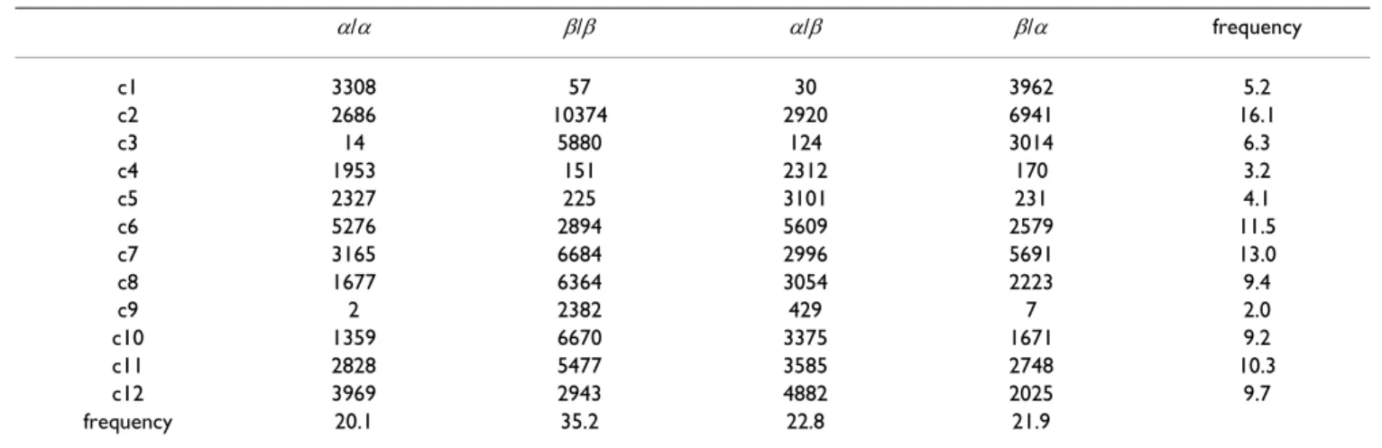
These two groups have the same organization: two states are connected to secondary structure exit states (c4 and c5 after a helix exit state and c2 and c3 after a strand exit state), one state is a "core" state, c6 for the first group and c8 for the second group, and two states lead to a secondary structure entry state (cl and c12 to the helix entry state, and c9 and c10 to the strand entry states). These two groups are relatively independent, there is a weak direct connection between the two groups (through states c10 and c6) and an indirect connection through the hub state c11. These two groups seems to model different types of loop. To further analyze the specific usage of the states in different loop types, the paths through the coil states are analyzed for different kind of loops. Note that these paths are obtained with the Viterbi algorithm. Both amino-acid and secondary structure sequences are given as input to OSS-HMM: in a way similar to the estimation of labeled sequence of secondary structures [31], it is possible to monitor the Viterbi algorithm using the product of amino-acid and label emission parameters instead of the amino-acid emissions only. The protein sequence and the label sequence are considered to be independent emis-sions by the same hidden process. In that case, the Viterbi algorithm computes the most probable trajectory in the hidden Markov Model, given the real secondary structure of the protein. Hence, it is not a secondary structure pre-diction, but the analysis of protein sequences using OSS-HMM. We then collect the number of times each coil state is observed in the four different classes of loops: α/α, β/β, α/β and β/α. The data obtained on the cross-validation set are shown in Table 2.

The repartition of the coil states indicates that the hidden states are preferentially found in particular loop types. For example, state c6 is observed 5256 times in a/a loops and only 2894 in β/β loops, although α/α loops represent 20.1% of the data, and the β/β loops represent 35%. To take into account this non-uniform repartition of differ-ent loop types, Table 2 is then submitted to a correspond-ence analysis. The data projection on the first two axes is shown on Figure 2. The first two axes respectively explain 66% and 32% of the variance. As shown by Figure 2, the first axis differentiate loops found after an helix (α/α and α/β) on one hand, and loops found after a strand (β/β and β/α) on the other hand. It means that, according to the hidden state usage, α/α or α/β differ from β/β or β/α loops. The data projection confirms the observations made from Figure 1: states c4, c5, c6 and c12 appear clearly associated to α/α loops and states c2, c3, c8, c9 and c10 to β/β loops. When projected on the first axis, state c1 appears close to the α/α type.

As shown on Figure 1 states c11 and, to a lesser extend c7, act as "hubs", allowing to switch between α/α and β/β loops. They are located near the origin on the

correspond-ence plot. States of the coil box show a marked tendency to favor particular amino acids: glycine for states c5, c8 and c9 and proline for states c12, and c2.

Comparison with available data in the literature

Several authors studied the sequence specificities of helix termini [32-35]. A direct comparison with these previous studies is not straightforward for several reasons. First, sec-ondary structure boundaries must be the same. As we showed in a previous study [36], the boundaries of helices and strands are the main point of disagreement between different secondary structure assignment methods. For instance, in their study Kumar and Bansal [33] re-assigned helix boundaries (based on DSSP assignment) using geo-metrical criteria. Thus, the reader should keep in mind that eventual discrepancies might occur because the refer-ence assignment is different (see for example ref. [35] that addresses this particular problem). Secondly, these previ-ous studies often revealed some general trends, whereas our model found several states for helix termination. The computation of general trends leads to the attenuation of the information because they average different signals. Previous studies [32-35] showed that amino-acid prefer-ences vary according to the position (begin/middle/end) in helices. Our model shows a directional progression in the hidden state graph in agreement with this feature. Aurora and Rose [32] found that PQDE are preferred at the first positions of alpha-helices. The helix starter H3 in our model shows a preference for proline residues, and H10, the second state in helix favors residues D and E. Kumar and Bansal identified a clear preference for resi-dues GPDSTN at positions preceding a helix [33]. It was confirmed in a recent study [35] in which Gibbs-sampling and helix shifting were used to reveal amino-acid prefer-ence in conjunction with a potential re-definition of helix termini. The idea was to allow a shift in the helix assign-ment, to maximize the sequence specificity of helix-cap.

In our model, the pre-helix state c1 favors residues D, S, T and N (weakly G). State c12, that also leads to the helix box, has a strong preference for Proline.

A typical motif of C-terminal capping in helices is the ter-mination of an helix by a glycine residue [37]. This feature has also be learned by OSS-HMM, since state c5, that fol-lows an helix, shows a strong preference for glycine. More precisely, Aurora and Rose identified several structural motifs of helix capping, corresponding to distinct sequence signatures [32]. This is in agreement with OSS-HMM since several helix states with different features (e.g. H4 and H6) can terminate an helix, and lead to several coil states (c11, c5, c4).

Engel and DeGrado showed a very clear periodicity of amino-acid distribution in helix cores: alternation of resi-dues with opposite physico-chemical properties every 3 or 4 residues [34]. This corresponds to the well-known model of amphipatic helices. Such helices are found at the interface between protein core and protein surface. One face, thus, bears polar residues and the other face hydro-phobic ones. Several cycles appear in the helix core in OSS-HMM: H2/H9/H1 (with possibly H8), H12/H4/H15 and H15/H11/H5/H13. The succession of H12 (hydro-phobic), H4 (polar) and H15(polar) fits well with the amphipatic model, as well as the succession H15(polar), H11 (hydrophobic), H5(hydrophobic) and H13(polar). Although in our model, amino-acids are independent, the periodicity of helices has been learned by the model, via the hidden structure.

Preferences at strand ends have not been well character-ized in the literature. Interestingly, OSS-HMM revealed alternate polar (b3, b7) or apolar (b5) starters of β -strands, as well as alternate polar (b2, b9) or apolar (b4) terminators. This could explain why sequence signatures are weak for strand-capping. If several capping motifs with Table 2: Occurences of coil states in different types of loops in the Viterbi paths of the cross-validation data set

α/α β/β α/β β/α frequency c1 3308 57 30 3962 5.2 c2 2686 10374 2920 6941 16.1 c3 14 5880 124 3014 6.3 c4 1953 151 2312 170 3.2 c5 2327 225 3101 231 4.1 c6 5276 2894 5609 2579 11.5 c7 3165 6684 2996 5691 13.0 c8 1677 6364 3054 2223 9.4 c9 2 2382 429 7 2.0 c10 1359 6670 3375 1671 9.2 c11 2828 5477 3585 2748 10.3 c12 3969 2943 4882 2025 9.7 frequency 20.1 35.2 22.8 21.9

opposite sequence signature co-exist, a global study would conclude to the lack of signature, because several signals are averaged. Our model exhibits several two state cycles that allows the alternation of hydrophobic and polar residues. This alternation has been pointed out in previous studies [38], it reflects the alternation of polar/

non-polar environments of residues in β-strands at the protein surface.

The path through the four states c3, c2, c8 and c10 allows the connection between two strands. Amino-acid ences are respectively (G, D, N), (P), (G) and (no

prefer-Principal component analysis of the association between hidden states and loop type

Figure 2

Principal component analysis of the association between hidden states and loop type. Data are obtained from the Viterbi decoding using secondary structure labeling on the cross-validation data.

ence). The propensities of c3, c2 and c8 fit well with the overall turn potentials identified by Hutchinson and Thornton [39] at position i, i + 1 and i + 2 of turns. How-ever, state c10 has no clear amino acid preference. The correspondence analysis indicates that some states are preferentially used in certain loop type. Previous studies have also revealed that sequence signatures differ accord-ing to the loop type [40]. Much like the hydrophobic/ polar alternation in amphipatic helices, HMMs can take into account such non strictly local correlations, by spe-cializing hidden states according to the hidden states to which they lead, instead of the amino-acids they emit, and the resulting amino-acid sequence bears non strictly local correlations. Amino-acid emissions are independent but they are conditioned with respect to the hidden process. OSS-HMM provides a new framework for the analysis of protein sequences: for example, the paths within the hid-den Markov model could be used to cluster the sequences. It would be particularly interesting to correlate the path based classification with known properties of the struc-tures such as SCOP folds. Preliminary results indicate however that a straightforward classification of the paths is not sufficient [see Additional file 5].

Use of OSS-HMM for generating protein sequences

Hidden Markov models can be used to generate amino acid sequences that are compatible with the underlying model. OSS-HMM is thus useful in bioinformatics appli-cation where simulated protein sequences are needed. For example, in protein threading analysis it is necessary, in order to assess the score significance, to use protein sequences to obtain an empirical score distribution [41]. A simulation study was carried on using OSS-HMM, indi-cating that simulated sequences share similar amino-acid composition with real protein sequences [see Additional file 3]. Concerning the length distribution of secondary structure elements, as no explicit constraint is integrated in the model, simulated sequences contain more very short segments than real sequences. More sophisticated models, i. e. semi-HMM, are needed to allows an explicit

modeling of the length of stay in the hidden states (Aydin et al [22]).

Secondary structure prediction with OSS-HMM

Evaluation on the independent test set

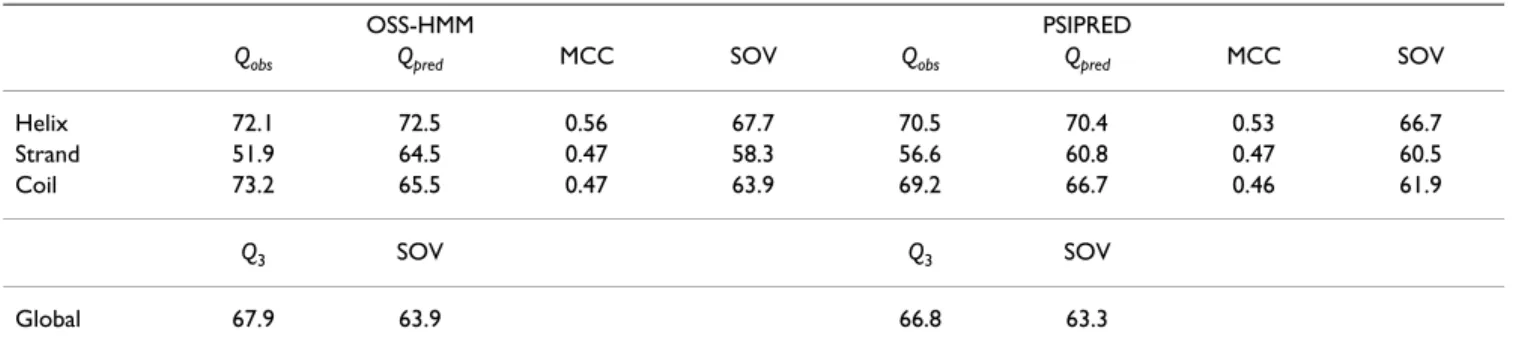
The prediction performance of OSS-HMM is evaluated on an independent test set of 505 protein sequences that were never used for training or model selection. These sequences share no more than 25% sequence identity with the sequences of the cross-validation data set and between sequence pairs; they constitute an appropriate evaluation data set. Prediction is done using a single sequence as input. To compare with existing methods, prediction are also done with the PSIPRED program (ver-sion 2.45) [4], using the single-sequence mode. This method is based on neural networks and sequence pro-files generated by PSI-BLAST. Here, PSI-BLAST is not used. Prediction scores obtained with OSS-HMM and PSIPRED are presented in Table 3. Here, the Q3 score is computed

on a per-residue basis. The Q₃ score obtained by OSS-HMM is 67.9% and 66.8% with PSIPRED. Due to its limited number of parameters, OSS-HMM exhibits no over-fit-ting: during the cross-validation, we obtained a mean per-residue Q₃ score of 67.9% on the data used to train the model, and 67.6% on the data not used to train the model (data not shown).

As can be seen from the various scores reported, OSS-HMM is very efficient concerning α-helix prediction, with a MCC of 0.56, but less efficient for β-strand and coil pre-diction, with MCC equal to 0.47. The low Q_obs (sensitivity) of β prediction, 51.9%, and high Q_obs for coil prediction, 73.2%, indicate that coils are frequently predicted instead of β-strands. This difficulty to predict β-strands is a known problem of secondary structure prediction method, prob-ably due to the non-local component of β-sheet forma-tion. It is difficult, with a HMM, to take into account this kind of long-range correlation with a model that has a rea-sonable number of parameters. We tried to integrate a non-local information in the prediction, without any sig-nificant amelioration (data not shown).

Table 3: Prediction accuracy obtained for the 505 sequences of the independent test set, using single sequences

OSS-HMM PSIPRED

Q_obs Q_pred MCC SOV Q_obs Q_pred MCC SOV Helix 72.1 72.5 0.56 67.7 70.5 70.4 0.53 66.7 Strand 51.9 64.5 0.47 58.3 56.6 60.8 0.47 60.5

Coil 73.2 65.5 0.47 63.9 69.2 66.7 0.46 61.9

Q3 SOV Q3 SOV

Global 67.9 63.9 66.8 63.3

Comparison with PSIPRED prediction scores shows that OSS-HMM offers a global Q₃ score of more than one point above PSIPRED score (67.9 vs 66.8%). Such a small differ-ence has to be statistically tested for significance. Since the variances of Q₃ scores per protein obtained by OSS-HMM and PSIPRED were not equal, as assessed by a F-test, the Welch test was used to compare them. The test is signifi-cant at the 5% level, we then conclude that OSS-HMM is more efficient than PSIPRED for the single-sequence based prediction. The detailed scores indicate OSS-HMM is better than PSIPRED for helix prediction, both in sensi-tivity and selecsensi-tivity. PSIPRED detects more β-strand – Q_obs is 56.6%, vs 51.9% for OSS-HMM – but is thus less specific – Q_pred is 60.8 vs 64.5% for OSS-HMM.

Testing against EVA dataset

We also tested the prediction accuracy on a dataset of 212 protein sequence from the EVA website. This dataset has been used to rank several secondary structure prediction methods and was the largest available at this time. Using homologous sequence information, the top-three meth-ods on this dataset were:

1. PSIPRED [4]: Q₃ = 77.8%,

2. PROFsec (B. Rost, unpublished): Q₃ = 76.7%, 3. PHDpsi [5] : Q₃ = 75%.

We ran the prediction on the 212 sequences, again using single sequences only, with OSS-HMM and PSIPRED. The per-sequence Q₃ scores achieved for each protein chain, by PSIPRED and OSS-HMM, are shown on Figure 3.

EVA dataset includes 20 membrane protein chains : 1pv6:A, 1pw4:A, 1rhz:A, 1zcd:A, 1zhh:B, 2a65:A, 1q90:N, 1q90:L, 1q90:M, 1s51:I, 1s51:J, 1s51:L, 1s51:M, 1s51:T, 1s51:X, 1s51:Z, 1rh5:B, 1rkl:A, 1u4h:A and ls7b:A. As can be seen on Figure 3, PSIPRED achieves good prediction for membrane proteins, whereas the prediction is rather poor with the HMM. Membrane proteins have amino acid propensities very different from those of globular pro-teins. As membrane proteins were excluded from the learning set to train the HMM, it is not surprising that their HMM-based predictions are largely incorrect. When these 20 sequences are excluded, the global Q₃ score on the remaining 192 proteins is 68.9% for PSIPRED and 68.6% for OSS-HMM, computed on 20 539 residues. EVA data set also contains very short sequences : 42 sequences are shorter than 50 residues. On very short sequence, a different prediction for a few residues has dra-matic consequences on the Q₃ score per protein, as shown on Figure 3. Proteins shorter than 50 residues are plotted in gray, they are responsible for the great dispersion of the

data. Some rather short sequences are shown in the plot: 1ycy (62 residues), 1r2m (70 residues), 1zeq:X (84 resi-dues), 1zv1A (59 resiresi-dues), 1r4g:A (53 residues). The mean length of a sequence in the EVA dataset is 189 resi-dues, and 212 residues in the independent test set. The protein length distribution of EVA dataset is shifted toward short sequences when compared to the length dis-tribution in the independent test set (data not shown). In order to analyze the effect of short sequences, and keep sufficient data, a Q₃ score is computed on the "core" of the protein sequences: the five terminal residues of each sequence are excluded from the computation. The global Q₃ score on the "core" of sequences are 68.1% for psipred and 69.2% for OSS-HMM.

This analysis indicates that the performance observed on our independent test set and the EVA dataset both con-clude to a better single-sequence based prediction using our OSS-HMM.

Confidence scale for the prediction

The posterior probabilities obtained for each structural class can be used as a confidence scale. In Figure 4, we show the per-residue Q₃ scores computed on the independ-ent test set, for residues with posterior probability lying in a given range. As can be seen, the correlation is excellent between posterior probability and the rate of good predic-tion: residues with high probabilities are better predicted. Thus, the posterior probability given by OSS-HMM is a good indicator of the confidence in the prediction. Influence of the secondary structure assignment software

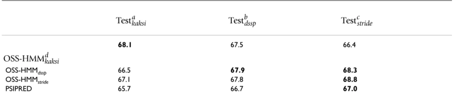
During the development of our method, several second-ary structure assignment methods were tested, both for HMM training and during the prediction evaluation. We tested the STRIDE [42], and KAKSI methods [36]. In Table 4, we report the per-residue Q₃ obtained with three flavors of OSS-HMM trained with KAKSI, DSSP and STRIDE assignments, and PSIPRED, when compared to secondary structure assignments provided by KAKSI, DSSP and STRIDE.

Not surprisingly, a better accuracy is achieved by the HMM when the same assignment method is used for training and evaluation (the estimated standard deviation being 0.2, the Q₃ scores achieved by OSS-HMM_dssp com-pared to DSSP and STRIDE assignments are equivalent). In these cases, the Q₃ score of OSS-HMM is always higher than the Q₃ score of PSIPRED. It is interesting to note that STRIDE assignments seem to be easier to predict either by OSS-HMM or PSIPRED, even though PSIPRED was trained with DSSP assignments.

Comparison with other HMM-based methods

For a precise comparison of OSS-HMM with other HMM-based methods, the evaluation should be done on

identi-cal datasets and compared to the same reference assign-ment. Here, we will only discuss the reported accuracies; conclusion about the possible superiority of a method

Q₃ obtained for each protein of the EVA 212 dataset, by PSIPRED and OSS-HMM

Figure 3

Q₃ obtained for each protein of the EVA 212 dataset, by PSIPRED and OSS-HMM. Globular proteins are shown as triangles and membrane proteins as crosses. Proteins shorter than 50 residues are indicated with gray symbols. The diagonal where both PSIPRED and OSS-HMM Q3s are equal is shown as a dashed line. OSS-HMM refers to the HMM presented in this

article.

20

40

60

80

100

20

40

60

80

100

Q3 score psipred

Q3 score OSS−HMM

should be made very cautiously. The first methods that used HMM for protein secondary structure prediction, proposed by Asai et al [9], Stultz et al [10,11], and Gold-man et al [12-14] were tested on small datasets. Moreover, the data bank contents are continuously growing, which induces an automatic improvement of the predictive methods because more data are available for training. Thus, the comparison with Asai, Stultz, Goldman and coworkers is not straightforward.

Among recent methods, Brenner et al [17], using a hidden Markov model with a sliding window in secondary struc-ture, reported a Q₃ score of 66.4% on a dataset of 513 sequences, using single sequence only. This result was obtained using the 'CK' mapping of the 8 classes of DSSP into three: (H) = helix, (E) = strand, others = coil, because it yielded a better accuracy than the 'EHL' mapping (see Method section). Using an amino-acid sliding window and amino-acid grouping, Zheng observed a Q₃ score of 67.9% on a small dataset of 76 proteins [18]. Very recently, Aydin et al obtained some very good results with semi-HMM and single sequences: a Q₃ score of 70.3% [22]. Their assignment method was DSSP with the 'CK' mapping and a length correction to remove strands shorter than 3 residues and helices shorter than 5 residues,

whereas we use the 'EHL' mapping and no length correc-tion. With the 'EHL' mapping and no length correction, they reported a Q₃ score of 67.4%, which is less than our results with HMM, i. e. 67.9%. To explore the influence of the length correction, we evaluate the Q₃ score on the independent test set of 505 sequences, assigned by DSSP with the length correction. We obtained Q3 = 69.6%.

Thus, it seems that OSS-HMM is, at least as accurate, maybe better than the other methods based on HMM that use single sequences.

Prediction using multiple sequences

It is well established that the use of evolutionary informa-tion improves the accuracy of secondary structure predic-tion methods [4,5]. The optimal model OSS-HMM estimated on single sequences can be used to perform the prediction with several sequences without further modifi-cation: homologous sequences retrieved by a PSI-BLAST search are independently predicted and the predictions are merged afterward in a consensus prediction. The underlying hypothesis is that homologous sequence share the same secondary structure. An example of multiple sequence based prediction for the SCOP domain d1jyoa_ is shown on Figure 5. Using the sequence of dljyoa_, OSS-HMM achieves a Q₃ score equal to 68.5%. The region around residues 60 to 100, indicated by ellipses, is not correctly predicted. The true secondary structure in this region consists in a α-helix of 15 residues (h1), a β-strand of 5 residues (b1) followed by a very short helix, and a sec-ond β-strand of 8 residues (b2) (see segments highlighted by ellipses on Figure 5). Using the single sequence, h1 is predicted as two strand segments and a short helix and s1 and s2 are predicted as one long helix interrupted by one residue in strand. The PSI-BLAST search with the sequence of d1jyoa_ produced a set of 8 sequences. Independent predictions for the 8 sequences show that sequences 2 to 8 have a high probability associated with helix in the region of h1. In the same way, sequences 2, 3 and 7 are predicted correctly as strand in the region s1. Concerning strand s2, only sequences 2 and 7 get a correct prediction. In sequences 3 to 6 this region is predicted as a helix, but have a non negligible probability of strand. The sequence of d1jyoa_ is present twice in the set because it was retrieved by the PSI-BLAST search (sequence 1 on Figure 5). This has no influence on the consensus prediction because the Henikoff weighting scheme ensures that two similar sequences receive the same weight and that the removal of one sequence results in the remaining sequence having a weight that is the double. The Henikoff weights in this sequence family varies from 0.096 to 0.150. Sequences 2 and 7, that contain a correct predic-tion for s2, have large weights (0.146 and 0.150). The final Q₃ score with the multiple sequences is 79.2%.

Q₃ score as a function of the posterior probability value

Figure 4

Q₃ score as a function of the posterior probability value. The Q3 score is computed on the subset of residues that are predicted with probabilities in given ranges. The dis-tribution of residues in the probability ranges is shown as a gray bar-plot. The right axis is related to this distribution.

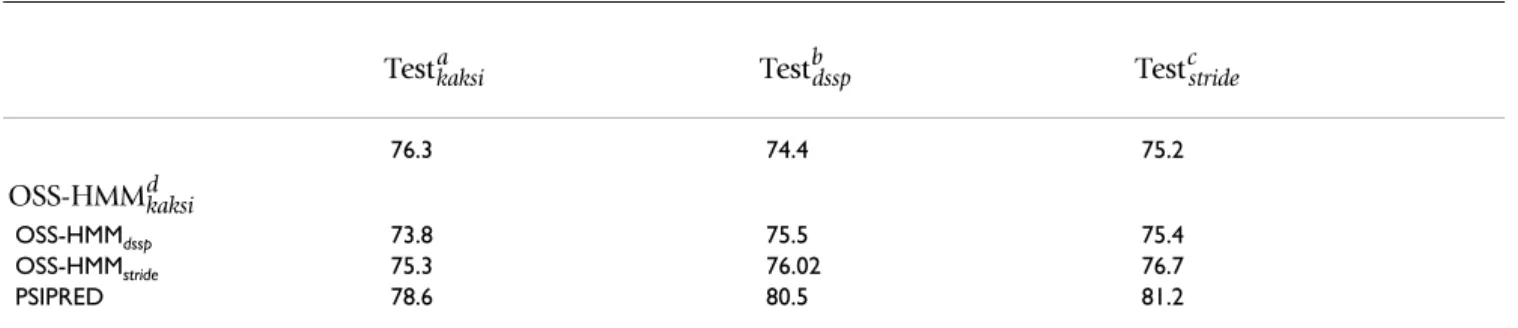
Table 5 reports the per-residue Q3 scores obtained by

OSS-HMM trained using various assignment methods, with different assignments taken as reference, on the 516 sequence of the independent test set. PSIPRED is also tested on this data set, using the same data bank for the profile generation. OSS-HMM achieves Q3 scores of 76.3,

75.5 and 76.7% using respectively KAKSI, DSSP and STRIDE assignments. PSIPRED outperforms OSS-HMM, whatever the assignment used for learning or evaluation with Q₃ scores ranging from 78.6 to 81.2%, depending on the assignment considered as the reference. It should be noted, however, that our HMMs were trained on single sequences and thus may be not optimal for multiple sequence prediction.

The detailed prediction scores of OSS-HMM trained on DSSP assignment and by PSIPRED are reported in Table 6. When compared to the single sequence-based prediction (Table 3), all the prediction scores have increased. α -heli-ces are still better predicted than strands and coil: the MCC is equal to 0.7 for helices vs 0.6 and 0.57 for strands and coil respectively. The sensitivity (Q_obs) of β-strand pre-diction is only 56.1%, for a specificity (Q_pred) of 80.3%: OSS-HMM predicts too few β-strands, but the β-strand prediction can be trusted. With single sequence, the sensi-tivity and specificity of β-strands of β-strand prediction were respectively equal to 51.9 and 64.5%. The inclusion of homologous sequence information thus greatly increased the specificity and moderately increased the sen-sitivity of the β-strand prediction. Previous studies based on HMM and multiple sequences reported global Q₃ scores of 74.3% by Bystroff et al [16], 72.2% by Brenner et al [17], and 72.8% by Chu et al [21]. Thus, our HMM pre-diction appears to be more efficient than the other meth-ods reported before, when used with homologous sequences. Moreover, our model is very parsimonious, i. e., has a very limited number of parameters when com-pared to complex models like the one of Bystroff et al, and neural networks.

In most of the methods that use evolutionary information with hidden Markov models, the likelihood and re-esti-mation formula are modified to incorporate the probabil-ity of a given profile in a hidden state. It is done using various formulation such as multinomial distribution [16,21,43], large deviation [17] or the scalar product of the emission parameters and the observed frequency (with a normalization to obtain a true probability) [44]. In all these cases, the estimation is done on a set of pro-files and the input for the prediction is a sequence profile. Another method, more closely related to ours, was pro-posed by Kall et al [45]. In this approach, the prediction is performed independently for each sequence. The predic-tions are then used as input for an "optimal accuracy" decoder that ensures that the predicted path is possible within the state graph. This method has the advantage of a satisfactory handling of gaps.

Here, we evaluated the predictive capability of our model, previously trained on single sequences, using a simple voting procedure. Since no strong constraints are applied to the paths within the graphs, we do not need sophisti-cated algorithm to be in agreement with the model struc-ture. Despite the simplicity of the multiple sequence procedure, the results are very promising: OSS-HMM appears to be as good, maybe more efficient, than previ-ous secondary structure prediction methods based on HMM that use evolutionary information. It would be very interesting to see if the explicit integration of sequence profiles for prediction and estimation as in [16,43,44] could increase the prediction accuracy.

Conclusion

In this paper we analyzed OSS-HMM, a model generated using an automated design [23], that allows the discovery of new features about the data. This method could in prin-ciple be applicable to other similar prediction problems, such as predicting transmembrane helices, splice sites, sig-nal peptides, etc. OSS-HMM has a limited number of parameters, which allows a biological interpretation of the state graph. Mathematically speaking, it is simple: a Table 4: Influence of the assignment method upon the Q₃ score obtained for the 505 sequences of the independent test set

68.1 67.5 66.4

OSS-HMMdssp 66.5 67.9 68.3

OSS-HMM_stride 67.1 67.8 68.8

PSIPRED 65.7 66.7 67.0

a_{: evaluation using KAKSI assignment,} b_{: evaluation using DSSP assignment,} c_{: evaluation using STRIDE assignment.} d_{: OSS-HMM}

x denotes 36 state

HMM trained using x assignment.

Test_kaksia Test_dsspb Test_stridec

Example of a multiple sequence prediction for d1jyoa_

Figure 5

Example of a multiple sequence prediction for d1jyoa_. Each plot represents the posterior probabilities of α-helix, β -strand and coil as a function of the position in the sequence, with the color scheme : magenta = helix, green = -strand, grey = coil. "Query" indicates the sequence of the initial sequence d1jyoa_ and "sequence 1" to "sequence 7" are the homologuous sequences retrieved by PSI-BLAST. The Henikoff weight of each sequence is indicated on each plot. "Consensus" indicate the consensus prediction for the sequence family. The predicted secondary structure in each case is shown as a colored bar in the upper part of each plot. The observed secondary structure of d1jyoa_ is plotted in the lower part of the figure. Ellipses focus on zones of the secondary structures that are modified in the prediction using only the query sequence and in the prediction using the multiple sequence alignment.

Q3=68.5% Q3=79.2% 0 20 40 60 80 100 120 0.0 0.4 0.8 weight=0.0963 Query 0 20 40 60 80 100 120 0.0 0.4 0.8 weight=0.0963 sequence 1 0 20 40 60 80 100 120 0.0 0.4 0.8 weight=0.146 sequence 2 0 20 40 60 80 100 120 0.0 0.4 0.8 weight=0.129 sequence 3 0 20 40 60 80 100 120 0.0 0.4 0.8 weight=0.140 sequence 4 0 20 40 60 80 100 120 0.0 0.4 0.8 weight=0.109 sequence 5 0 20 40 60 80 100 120 0.0 0.4 0.8 weight=0.133 sequence 6 0 20 40 60 80 100 120 0.0 0.4 0.8 weight=0.150 sequence 7 0 20 40 60 80 100 120 0.0 0.4 0.8 consensus

first order Markov chain for the secondary structure state succession (hidden process) and independent amino-acids, conditionally to the hidden process. Despite its sim-plicity, it is able to capture some high order correlations such as four-states periodicity in helices and even the spec-ification of distinct types of loops. In this kind of model, high order correlations are implicitly taken into account by the constraints on the transitions. OSS-HMM learned some classical features of secondary structures described previously in other studies: specific sequence signature of helix capping, sequence periodicity of helices and polar/ non polar alternation in β-strands. New features revealed by our model are the presence of several, well distinct amino acid preferences for β-strand capping. To the best of our knowledge, previous studies about β-strand specif-icities did not reveal such strong signatures.

Due to its limited number of parameters, no over-fitting was observed when using OSS-HMM for secondary struc-ture prediction. On single sequences, it performs better than PSIPRED and other HMM-based methods, with a Q₃ score of 67.9%. The use of the same model, OSS-HMM, in a multiple sequence prediction framework gave very promising results with a Q₃ equal to 75.5%. This level of

performance is as good, maybe better, than the previous methods based on HMMs and evolutionary information [16,17,21]. The perspectives of this work are twofolds. First, we can re-estimate the model and carry out the pre-diction using sequence profiles as done in [16,43,44]. A second perspective is the extension to the local structure prediction of non-periodic regions. Most methods predict protein secondary structures as 3 states: helix, strand and coil. Coil is a 'complementary' state for those residues that do neither belong to a helix nor to a strand, accounting for about 50% of all residues. Therefore predicting coils does not provide any information about the residue conforma-tions. One way of extracting more information from the protein sequence is to predict Φ/Ψ zones for coil residues. Such a prediction can be readily included in the HMM and we plan to use it for de novo prediction.

Methods

Data

The dataset is a subset of 2524 structural domains of ASTRAL 1.65 [46] corresponding to the SCOP domain definition [47]. An initial list of domains with no more than 25% identity within sequence pairs was retrieved on the ASTRAL web page [48]. This list is filtered in order to Table 6: Prediction scores obtained for the 505 sequences of the independent test set using multiple sequence information

PSIPRED

Qpred MCC SOV Qobs Qpred MCC SOV

Helix 78.5 83.3 0.70 77.5 85.3 85.9 0.77 85.0 Strand 56.1 80.3 0.60 65.1 76.1 78.2 0.70 78.9 Coil 83.8 68.4 0.57 70.8 78.6 76.9 0.63 71.5 Q₃ SOV Q₃ Global 75.5 72.0 80.5 78.6 a_{: OSS-HMM}

dssp denotes 36 state HMM trained using dssp assignment, b: predictions scores are reported with the dssp assignment taken as the

reference.

OSS-HMMdsspa

Q_obsb

Table 5: Q₃ scores obtained for the 505 sequences of the independent test set using multiple sequence information

76.3 74.4 75.2

OSS-HMMdssp 73.8 75.5 75.4

OSS-HMM_stride 75.3 76.02 76.7

PSIPRED 78.6 80.5 81.2

a_{: evaluation using kaksi assignment,} b_{: evaluation using DSSP assignment,} c_{: evaluation using STRIDE assignment.} d_{: OSS-HMM}

x denotes 36 state

HMM trained using x assignment.

Test_kaksia Test_dsspb Test_stridec

remove NMR structures, X-ray structures with a resolution factor greater than 2.25 Å, membrane proteins and domains shorter than 50 residues [see Additional file 6]. Secondary structures are assigned by DSSP [49], STRIDE [42] or KAKSI [36]. STRIDE and DSSP assignments are reduced to three classes using the 'EHL' mapping employed in EVA evaluation [3]: (H, G, I) = helix, (E, b) = strand, others (S, T, blank) = coil. The whole dataset con-tains 492 724 residues with a defined secondary structure. The dataset is divided into a cross-validation data set and an independent test set containing respectively 2019 sequences (397401 residues) and 505 sequences (95 323 residues). The independent test set is never used in param-eter estimation and model selection. Models are trained and tested using a four-fold cross-validation procedure on the cross-validation data.

Secondary structure contents are similar in the cross-vali-dation and the independent datasets: 38% helix, 22% strand and 40% coil according to STRIDE assignment and 37% helix, 23% strand and 40% coil according to DSSP assignment.

The method is also tested on a dataset of 212 protein sequences retrieved from the EVA website ("common sub-set 6" [50]). DSSP secondary structure assignment of the corresponding sequences were also retrieved on this web-site. This set of 212 protein sequences has been used to evaluate the prediction performance of the methods involved in EVA assessment.

Hidden Markov models

HMM applied to secondary structure prediction

Hidden Markov models are probabilistic models of sequences, appropriate for problems where a sequence is supposed to have hidden features that need to be pre-dicted. The strong theoretical background of HMM (see for example [51]) allows the estimation of model param-eters, and the prediction of the hidden features from the observed sequence. The secondary structure prediction task can be expressed in term of a hidden data problem as follows:

• the secondary structure of a particular residue along the sequence is a hidden process,

• the amino acid sequence is the observed process. The secondary structure succession is governed by a first order Markov chain and amino-acids are independent, conditionally to the hidden process.

In a very basic HMM, each secondary structure is modeled by a single state. The parameters of the model are the tran-sition and emission probabilities. Here, we will consider more complex models with several hidden states per sec-ondary structure. The difficulty is to choose the optimal number of hidden states for each secondary structure. Model parameters are then estimated from available data. HMM training

The number of hidden states for each secondary structure and initial parameter values are chosen as explained in the next section. Models are trained with labeled sequence of secondary structures [31] together with the amino-acid sequence using the Expectation-Maximization (EM) algo-rithm [51]. Secondary structures are labeled according to the DSSP assignment. Labels of secondary structure are removed for the prediction step. All models are trained and handled with the software SHOW [52], extended to handle protein sequences.

Optimal HMM selection

Models of increasing size are built without a priori knowl-edge. All transition probabilities are initially set to , N being the total number of hidden states. Initial emission parameters are randomly chosen. The similarity of models estimated on different data sets is checked [see Additional file 2]. Ten different starting point are used and the model with the best likelihood is selected during the EM estima-tion. For large models, 100 starting points are used to ver-ify that the EM estimation has sufficiently explored the parameter space. This procedure provided results similar to those obtained with 10 starting points. The optimal models are then selected using three criteria:

• prediction accuracy assessed by the Q₃ score,

where N_ij denotes the number of residues in structure i predicted in structure j, and N_tot the total number of resi-dues,

• Bayesian Information Criterion [53] that ensures the best compromise between the goodness-of-fit of the HMM and a reasonable number of parameters,

BIC = logL - 0.5 × k × log(N),

where logL denotes the log-likelihood of the learning data under the trained model, k is the number of independent model parameters and N is the size of the training set. k is

1 N Q N N ii i tot 3=

∑

the actual number of free parameters in the final model, i. e., parameters estimated to be null are not counted. The first term of BIC increases with the number of parameters; it is penalized for parsimony by the second term. BIC cri-terion does not take prediction accuracy into account. • the statistical distance between two models as described by Rabiner [51]. The symmetric distance D_s between two models M1 and M2 is given by:

where O(2) _{is a sequence of length T generated by model}

M₂ and log L(O(2)_|M

i) is the log-likelihood of O(2) under model M_i.

Briefly, the selection is done as follows (see [23] for fur-ther details about the selection procedure). Initially, mod-els with equal number of hidden states for each structural class are considered. The three above criteria help select-ing models with a limited number of hidden states, about 15 per structural class. Then we consider models for which the number of states increases for one structural class while it remains fixed to one for the two other classes. This defines the model size range that needs to be explored for each structural class: 12 to 16 states for helices, 6 to 10 states for strands and 5 to 13 states for coil. Finally, all 225 models within these size ranges are generated and evalu-ated. The optimal model, described in the result section, has 36 hidden states: 15 for helices, 9 for strands and 12 for coil. We will refer to this model as OSS-HMM. HMM prediction using single sequences

Predictions are done using the forward/backward algo-rithm. This allows the computation of the posterior prob-ability of each hidden state in each position of the query sequence, given the model and the whole sequence: P(S_t = u | X), where S_t is the hidden state at position t, u is a par-ticular hidden state and X is the amino-acid sequence (see, e.g., [54] for computation detail).

The posterior probability of hidden states of the same structural class c are summed together:

c being the set of hidden states modeling the structural class. The structural class with the highest probability is predicted.

HMM prediction using multiple sequences

Models estimated with single sequences can be used in a framework of a multiple sequence prediction. The multi-ple sequence based prediction is carried out in three steps: 1. a PSI-BLAST search is performed using the sequence to be predicted, resulting in a family of n homologous sequences,

2. the secondary structures of these n sequences are inde-pendently predicted using the HMM,

3. the n predictions are combined into a unique predic-tion.

In the first step, homologous sequences are extracted using PSI-BLAST with search parameters -j 3 -h 0.001 -e 0.001, against a non-redundant data bank. The redun-dancy level of the data bank is 70% (i.e., no pair of sequences has more than 70% identical residues after alignment) and the data bank has been filtered to remove low-complexity regions, transmembrane regions, and coiled-coil segments. Other data banks (80 and 90% redondancy level, filtered or not) were tested and the above choice provided the best results. In the second step, n predictions are performed, independently for each sequence retrieved in the first step, with the forward-back-ward algorithm.

In the third step, the n independent predictions are com-bined. At each position of the sequence family, the predic-tions of the n sequences for the same position contribute to the final prediction, with a sequence weight. Sequence weights are used to correct for the fact that the n sequences retrieved in the first step do not necessarily correctly sam-ple the sequence space. For examsam-ple, a sequence family can be composed of several very similar sequences and a few more distant sequences. Without sequence weights, the final prediction would be biased toward the set of sim-ilar sequences and the information carried by the more distant sequences would be lost. The probability of the secondary structure s at the position t of the sequence fam-ily F is then given by:

where P_i (S_t = s) is the posterior probability of the second-ary structure s obtained for the single sequence i at posi-tion t (see equaposi-tion 1). The sum is taken over all the n sequences retrieved for the family that do not contain gap at the considered position. The secondary structure with the highest probability is taken as the prediction.

D M M D M M D M M D M M T L O M L s( , ) ( , ) ( , ) ( , ) | log ( ( )| ) log 1 2 2 1 1 2 2 1 2 1 2 1 = + = − ((O( )2 |M₂) | P S_t s X P S_t u X u c ( = | )= ( = | ),

( )

∑

( )

∑

Several weighting scheme were tested: Henikoff weights [55], a weighting scheme introduced by Thompson et al [56] that uses phylogenetic trees, and a new weighting scheme based on information sharing in phylogenetic trees [see Additional file 4].

We also developed a more sophisticated multiple sequence prediction in which the HMM is fed with the sequence families and the corresponding phylogenetic trees [see Additional file 4]. In this case, it is supposed that aligned sequences not only share the same secondary structure but the same path of hidden states.

The best results were obtained using Henikoff weighting scheme and are presented in the Result section.

Assessing the prediction

Accuracy of secondary structure prediction is assessed using standard scores such as Q₃, SOV [57], Q_obs (sensitiv-ity), Qpred (specificity) and Matthew's correlation coeffi-cient [see Additional file 1].

Availability and requirements

Project name:

OSS-EMM Project home page:

http://migale.jouy.inra.fr/mig/mig_fr/servlog/oss-hmm Operating system: Linux Programming language: C++, perl, python. Other requirements:

GSL library (1.3 or higher, http://www.gnu.org/software/ gsl/gsl.html).

Licence:

GNU GPL

Any restrictions to use by non-academics:

no.

Authors' contributions

JM conceived the models and carried out the analysis. JM, JFG and FR conceived the study and participated in its

design and coordination. All authors read and approved the final manuscript.

Additional material

Acknowledgements

We would like to acknowledge Anne-Claude Camproux, Alexandre de Brevern and Catherine Etchebest from EBGM for helpful discussions during the redaction of the manuscript, and Pierre Nicolas from MIG who devel-oped the SHOW software. We thank Claire Guillet and Emeline Legros for their contribution to the work presented in additional file 4. We are grate-ful to INRA for awarding a Fellowship to JM. This research was funded in part by the 'ACI Masse de données – Genoto3D project'.

References

1. Karchin R, Cline M, Mandel-Gutfreund Y, Karplus K: Hidden Markov models that use predicted local structure for fold

Additional file 1

Definition of prediction scores. Definitions of Q3, Qobs, Qpred, MCC and SOV scores.

Click here for file

[http://www.biomedcentral.com/content/supplementary/1472-6807-6-25-S1.pdf]

Additional file 2

Comparing hidden Markov models. Elements about the problem of com-paring HMMs to ensure that the model is interpretable.

Click here for file

[http://www.biomedcentral.com/content/supplementary/1472-6807-6-25-S2.pdf]

Additional file 3

Simulation study. Analysis of amino-acid composition of sequences that are simulated with OSS-HMM and a comparison to real data. Click here for file

[http://www.biomedcentral.com/content/supplementary/1472-6807-6-25-S3.pdf]

Additional file 4

Handling homologs with HMM. Overview of other approaches we devel-oped to integrate evolutionary information in the prediction.

Click here for file

[http://www.biomedcentral.com/content/supplementary/1472-6807-6-25-S4.pdf]

Additional file 5

Classification of protein sequences using paths in the HMM. Attempt to classify protein sequences using their paths in OSS-HMM.

Click here for file

[http://www.biomedcentral.com/content/supplementary/1472-6807-6-25-S5.pdf]

Additional file 6

URL to retrieve the domain lists. Url to retrieve the cross-validation and test data sets.

Click here for file

[http://www.biomedcentral.com/content/supplementary/1472-6807-6-25-S6.pdf]