HAL Id: tel-00968069
https://tel.archives-ouvertes.fr/tel-00968069
Submitted on 31 Mar 2014HAL is a multi-disciplinary open access archive for the deposit and dissemination of sci-entific research documents, whether they are pub-lished or not. The documents may come from teaching and research institutions in France or abroad, or from public or private research centers.
L’archive ouverte pluridisciplinaire HAL, est destinée au dépôt et à la diffusion de documents scientifiques de niveau recherche, publiés ou non, émanant des établissements d’enseignement et de recherche français ou étrangers, des laboratoires publics ou privés.
Development of an energy efficient, robust and modular
multicore wireless sensor network
Hong-Ling Shi
To cite this version:
Hong-Ling Shi. Development of an energy efficient, robust and modular multicore wireless sensor network. Other [cs.OH]. Université Blaise Pascal - Clermont-Ferrand II, 2014. English. �NNT : 2014CLF22435�. �tel-00968069�
N° d’ordre : D. U. 2435
EDSPIC : 641
UNIVERSITÉ BLAISE PASCAL - CLERMONT ІІ
ÉCOLE DOCTORALE DE
SCIENCES POUR L’INGÉNIEUR DE CLERMONT-FERRAND
Thèse
Présentée par
Hong-Ling SHI
Pour obtenir le grade deDOCTEUR D’UNIVERSITÉ
Spécialité : INFORMATIQUE
Development of an Energy Efficient, Robust and Modular
Multicore Wireless Sensor Network
Soutenue publiquement le 23 janvier 2014 devant le jury :
Directeur de la thèse :
Prof. Kun Mean HOU
Membres du jury :
Prof. Bernard Tourancheau (University of Joseph Fourier, rapporteur) Prof. Houda Labiod (ENST ParisTech, rapporteur)
Prof. Alain Quilliot (UBP, examinateur)
Dr. Jean-Pierre Chanet (IRSTEA, examinateur) Prof. Jorge Garcia-Vidal (UPC, examinateur) Dr. Jianjin LI (invité)
Remerciements
First and foremost, I would like to thank my supervisor, Prof. Kun Mean HOU, who gave me an opportunity to do this challenging and interesting research. He is a constant source of inspiration and always helpful when I need help. I learned so such from him and I believe these unforgettable experiences and valuable knowledge will be a great asset in my future careers as well as in my personal life.
I would like to thank Conseil Régional d’Auvergne and Feder for their financial support. I would also like to thank Laboratory LIMOS- UMR 6158 - Université Blaise Pascal/CNRS for providing all necessary equipment to do the research.
I am very grateful to all the members of the jury for their valuable time and feedback. I am very thankful to Prof. Hong SUN from Wuhan University (China) for her recommendation and encouragement. I am very grateful to Dr. Jian-Jin LI and Dr. Christophe DE VAULX for their kind help, patience and support. I am thankful to Prof. Haiying ZHOU and Prof. XiaoZhong YANG from Harbin Institute of Technology (China) for the in-depth discussions with them.
I would like to express many thanks to present and former team members of SMIR group for their efficient cooperation and kind help. Thanks to XunXing DIAO, Hao DING, Xing LIU, YiBo CHEN, Bin TIAN, Peng ZHOU, Khalid el GHOLAMI, Muhammad YUSRO, Lizhong ZHANG, Zuoqin HU, Messaoud KARA, XinChen ZHANG and Jing WU. They have all contributed to create a great work environment.
Finally, I would like to dedicate this dissertation, in loving memory, to my father. May his soul rest in peace! I would also like to dedicate this dissertation to my mother for her support, encouragement, and love over the years. I would also like to thank my sister, my brother, and all my friends who have supported me. Last, but not least, my deepest gratitude is towards my wife, Li-Li HUANG, for her love, patience, and support.
Table of Contents
Table of Contents ... iii
List of Figures ... ix
List of Tables ... xi
List of Acronyms ... xiii
Chapter 1.
Introduction ... 1
1.1.
Motivation and Problem Statement ... 1
1.2.
Our Multicore Solutions ... 3
1.3.
Contributions ... 5
1.4.
Dissertation Structure ... 5
Chapter 2.
General Purpose Dependable System ... 7
2.1.
Introduction ... 7
2.1.1. Dependability Attributes ... 8
2.1.2. Dependability Threats ... 9
2.1.3. Dependability Means ... 9
2.2.
Dependability Evaluation Techniques ... 10
2.2.1. Dependability Terms ... 10
2.2.2. Dependability model types ... 14
2.2.3. Dependability computation methods ... 15
2.3.
Fault Tolerance and Redundancy ... 16
2.3.1. Space Redundancy ... 16
2.3.2. Time Redundancy ... 17
2.4.
MTBF Values Evaluation ... 18
2.5.
RAS of Computer System ... 20
2.6.
Summary ... 22
Chapter 3.
Dependability of Wireless Sensor Networks ... 23
3.1.
Wireless Sensor Networks ... 23
3.1.2. WSN Nodes ... 24
3.1.3. WSN Applications ... 29
3.2.
Major Dependable Challenges ... 33
3.2.1. Application Requirement ... 33
3.2.2. Dependability Threats ... 33
3.2.3. Resource Constraint ... 34
3.3.
Current Dependable Approaches ... 34
3.3.1. Current Approaches ... 34
3.3.2. TMS570 Safety MCU ... 35
3.4.
Observations of Real World WSN Deployments ... 36
3.5.
Summary ... 36
Chapter 4.
Multicore WSN Node Architecture... 37
4.1.
Introduction ... 37
4.2.
Multicore WSN Node Architecture ... 38
4.2.1. Generalized Multicore Architecture ... 38
4.2.2. Functional Safety Mechanism ... 39
4.2.3. Fault-tolerant Mechanism ... 40
4.2.4. Resource-aware Mechanism ... 40
4.2.5. Dissymmetrical Multicore Structure ... 42
4.3.
Different Type of Cores ... 43
4.3.1. IGLOO nano FPGAs ... 43
4.3.2. 4-bit NanoRisc ... 44
4.3.3. 8-bit ATMEGA1281 ... 44
4.3.4. 8-bit RISC core microcontroller AVRRF ... 45
4.3.5. 32-bit RISC core microcontroller AT91SAM7Sx ... 45
4.3.6. Raspberry Pi Board ... 45
4.3.7. PandaBoard ES Board ... 46
4.3.8. ARM CortexTM-M3 Based Microcontroller ... 47
4.3.9. Summary ... 48
4.4.
HSDTVI Interface ... 48
4.4.2. HSDTVI Architecture ... 49
4.4.3. Different Scenario of the HSDTVI Implementation ... 50
4.4.4. Summary ... 57
4.5.
Summary ... 58
Chapter 5.
High Reliability Design Process dedicated to Resource
Constraint Embedded System ... 59
5.1.
Introduction ... 59
5.2.
Traditional Design Process Models ... 59
5.2.1. Waterfall Model ... 60 5.2.2. V Model ... 60 5.2.3. Incremental Model ... 61 5.2.4. Spiral Model ... 62 5.2.5. RAD Model ... 63 5.2.6. Agile Model ... 64 5.2.7. Summary ... 65
5.3.
High Reliability Design Process Based on Multicore Architecture .... 66
5.3.1. General Overview ... 66
5.3.2. Model-Driven Engineering ... 66
5.3.3. Model of Multicore WSN Architecture ... 68
5.3.4. Early Validation of Requirement ... 71
5.3.5. Design for Multicore Run Time Testability ... 74
5.3.6. Fault Injection ... 75
5.4.
Summary ... 78
Chapter 6.
Implementation of Multicore WSN Node ... 79
6.1.
E²
MWSN: High Reliability and High Performance Multicore WSN
Node 79
6.1.1. General Overview ... 796.1.2. Hardware Architecture ... 80
6.1.3. Key Features ... 82
6.1.4. Performance ... 82
6.2.1. General Overview ... 86
6.2.2. Hardware Architecture ... 87
6.2.3. End-Device Sleep & Wakeup Work Mode ... 88
6.2.4. Key Features ... 90
6.2.5. Performance ... 90
6.3.
SIS: High Reliability Sensor Node in Smart Irrigation System ... 92
6.3.1. General Overview ... 92
6.3.2. Hardware Architecture ... 93
6.3.3. Key Features ... 94
6.3.4. Performance ... 95
6.4.
iLiveEdge: High Reliability and Multi-Support Multicore WSN Edge
Router 97
6.4.1. General Overview ... 976.4.2. Hardware Architecture ... 98
6.4.3. Key Features ... 99
6.4.4. Performance ... 99
6.5.
EPER: Highest Performance High Reliability and Multi-Support
Multicore WSN Edge Router ... 100
6.5.1. General Overview ... 100
6.5.2. Hardware Architecture ... 101
6.5.3. Key Features ... 102
6.5.4. Performance ... 103
6.6.
RPiER: Higher Performance High Reliability and Multi-Support
Multicore WSN Edge Router ... 104
6.6.1. General Overview ... 104 6.6.2. Hardware Architecture ... 104 6.6.3. Key Features ... 105 6.6.4. Performance ... 106
6.7.
Related Projects ... 107
6.7.1. Precision Agriculture ... 1076.7.2. Smart Irrigation System ... 110
6.8.
Summary ... 114
Chapter 7.
Conclusion and Ongoing Work ... 117
7.1.
Conclusion ... 117
7.2.
Next Generation WSN node ... 118
7.2.1. Next Generation Multicore SoC for WSN node ... 118
7.2.2. Finite State Machine OS: FSMOS ... 124
7.3.
Perspective ... 128
Bibliography ... 131
RESUME ... 139
List of Figures
Figure 1-1 Overview of WSN applications(Yick et al., 2008) ... 2
Figure 1-2 Block diagram of DFT system... 3
Figure 1-3 Block diagram of Multicore WSN node ... 4
Figure 1-4 Block diagram of Multicore WSN node with redundancy for application core ... 4
Figure 2-1 The dependability tree (Algirdas Avizienis, Laprie, & Randell, 2001) ... 8
Figure 2-2 Typical evolution of failure rate over a lifetime of a hardware system (Dubrova, 2013) ... 11
Figure 2-3 Typical evolution of failure rate over a lifetime of a software system (Dubrova, 2013) ... 11
Figure 2-4 MTBF versus Lifetime ... 13
Figure 2-5 Reliability block diagram of a two-component system: (a) Serial, (b) parallel ... 14
Figure 2-6 MTBF Estimates for Intel® Server System R1208RPMSHOR (Intel Corporation, 2013a) ... 19
Figure 2-7 Laptop three years Failure Rates (SquareTrade, 2009) ... 19
Figure 2-8 Three Years Laptop Malfunction Rates by Manufacturer (SquareTrade, 2009) ... 20
Figure 2-9 IBM server system RAS operations (IBM Corp, 2012) ... 21
Figure 2-10 Advanced RAS features of an IBM System x3850 X5 server (IBM Corp, 2012) ... 21
Figure 3-1 Circuit Board of MICAz ... 24
Figure 3-2 Circuit Board of MICA2 ... 25
Figure 3-3 Circuit Board of Telos B ... 25
Figure 3-4 Circuit Board of IRIS ... 26
Figure 3-5 Circuit Board of Cricket ... 26
Figure 3-6 Block diagram of TI TMS570 microcontroller (Texas Instruments Incorporated., 2013) ... 35
Figure 4-1 Block diagram of TelosB ... 38
Figure 4-2 Block diagram of Multicore Architecture ... 39
Figure 4-3 Standby sparing system (Dubrova, 2013) ... 40
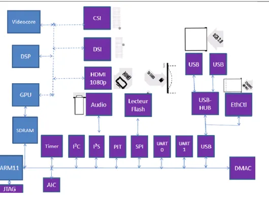
Figure 4-4 Block diagram of the Raspberry Pi Board ... 46
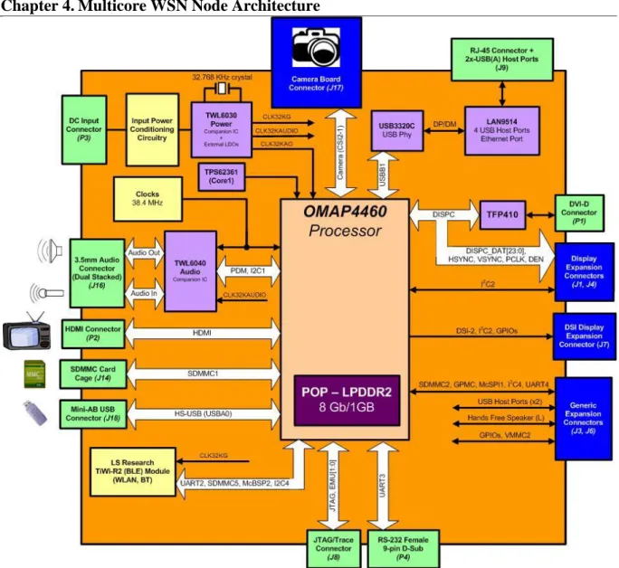
Figure 4-5 Block diagram of the PandaBoard ES Board (PandaBoard ES, 2013) ... 47
Figure 4-6 The HSDTVI Architecture... 50
Figure 4-7 The HSDTVI Interface used for Debug Mode Scenario ... 51
Figure 4-8 Circuit Board of HSDTVI used for Debug Mode Scenario ... 52
Figure 4-9 The HSDTVI Debug Trace and Validate Process ... 52
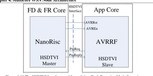
Figure 4-10 The HSDTVI Interface used for real-time Fault Detection Mode Scenario ... 54
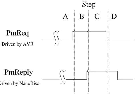
Figure 4-11 Timing diagram of AVR and NanoRisc Communication ... 55
Figure 5-1 Block diagram of Waterfall Model ... 60
Figure 5-2 The V-model of the Systems Engineering Process ... 61
Figure 5-3 The Incremental Model of Development... 62
Figure 5-4 The Spiral model of the Systems Engineering Process ... 63
Figure 5-5 The Rapid Application Development (RAD) Model ... 64
Figure 5-6 The Agile Development Model ... 65
Figure 5-7 Overview of Model Driven Engineering ... 67
Figure 5-8 Example Multicore WSN Architecture Diagram... 68
Figure 5-10 Early Validation Based on Virtual Processor Emulator ... 74
Figure 5-11 Block diagram of the Fault Injection TestBed ... 76
Figure 5-12 Circuit Board of the Fault Injection TestBed ... 76
Figure 6-1 Block diagram of the E²MWSN ... 80
Figure 6-2 Hardware Architecture of E²MWSN ... 80
Figure 6-3 Circuit Board of the E²MWSN ... 81
Figure 6-4 Measure Schematics of the E²MWSN ... 83
Figure 6-5 Block diagram of iLive ... 86
Figure 6-6 Hardware Architecture of the iLive ... 87
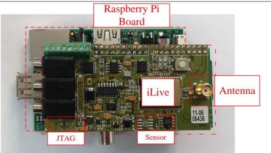
Figure 6-7 Circuit Board of iLive ... 88
Figure 6-8 Timing Diagram of iLive ... 89
Figure 6-9 Measure Schematics of the iLive ... 90
Figure 6-10 Block diagram of the SIS ... 92
Figure 6-11 Hardware Architecture of the SIS ... 93
Figure 6-12 Circuit Board of the SIS ... 94
Figure 6-13 Measure Schematics of the SIS ... 95
Figure 6-14 Block diagram of the iLiveEdge ... 98
Figure 6-15 Hardware Architecture of the iLiveEdge ... 98
Figure 6-16 CircuitBoard of the iLiveEdge ... 99
Figure 6-17 Block diagram of the EPER ... 101
Figure 6-18 Hardware Architecture of the EPER ... 102
Figure 6-19 Circuit Board of the EPER ... 102
Figure 6-20 Block diagram of the RPiER ... 104
Figure 6-21 Hardware Architecture of the RPiER ... 105
Figure 6-22 CircuitBoard of RPiER ... 105
Figure 6-23 Outdoor Experiment in ISIMA Garden ... 108
Figure 6-24 Real world Experiment in Montoldre (Cooperation with Irstea) ... 108
Figure 6-25 Heterogeneous Architecture of the MiLive ... 109
Figure 6-26 Circuit Board of the MiLive ... 110
Figure 6-27 Demo Web page of the MiLive platform ... 110
Figure 6-28 Demo Web page of the SIS Platform ... 111
Figure 6-29 Real World Long Term Online Demo of the SIS Platform ... 111
Figure 6-30 Block diagram of the SEE-stick ... 112
Figure 6-31 SEE-Stick Prototype ... 113
Figure 6-32 SEE-Stick Remote Monitoring Demo Web page ... 114
Figure 7-1 Architecture of Next Generation Multicore SoC ... 119
Figure 7-2 Uniform NanoRisc based on the Multicore SoC ... 120
Figure 7-3 Different Common Risc based on the Multicore SoC ... 121
Figure 7-4 FSMOS Modules based the Multicore SoC ... 122
Figure 7-5 Intra-Chip Multicore Interconnection Networks ... 123
Figure 7-6 Cross Platform of the FSMOS Software Architecture ... 126
List of Tables
Table 3-1 Comparison of common available scalar WSN Nodes ... 27
Table 3-2 Key Features of Low performance WMSN nodes ... 28
Table 3-3 Key Features of Medium performance WMSN nodes ... 29
Table 4-1 Key features of Different Core ... 48
Table 4-2 the HSDVTI Pin connections between AVR and Raspberry Pi Board ... 51
Table 4-3 The HSDVTI Pin connections between NanoRisc and AVR ... 54
Table 4-4 Pseudo Code for Heart Beat Checking of Coordinator ... 55
Table 4-5 Pseudo Code for Error Handle of the coordinator ... 56
Table 4-6 Pseudo Code for Heart Beat Checking of End-device ... 56
Table 4-7 Pseudo Code for Error Handle of End-device... 57
Table 5-1 Example Module List ... 69
Table 5-2 Example High-level Interface of cAVR Module ... 69
Table 5-3 Example High-level Interface of cEvDrv Module ... 70
Table 5-4 Sample Functional Specification of cEvDrv Module ... 71
Table 5-5 Fault Injection modes with contact ... 77
Table 5-6 Fault Injection modes without contact ... 78
Table 6-1 Operation modes of the E²MWSN ... 82
Table 6-2 Task Resource Required of the E²MWSN on single AT91SAM7Sx mode ... 83
Table 6-3 Task Resource Required of the E²MWSN on single ATMEGA1281mode ... 84
Table 6-4 Task Resource Required on AT91SAM7Sx plus ATMEGA1281 mode ... 84
Table 6-5 FIT of Each Core in the E²MWSN* ... 85
Table 6-6 MTBF/MTBCF of Each E²MWSN Operation Mode ... 86
Table 6-7 Default Timing Parameters of iLive ... 89
Table 6-8 Task Resource Required of iLive ... 91
Table 6-9 FIT of each core in the iLive* ... 91
Table 6-10 Task Resource Required of the SIS on Dry Soil * ... 95
Table 6-11 Task Resource Required of the SIS on Normal Soil ... 96
Table 6-12 FIT of Each core in the SIS* ... 97
Table 6-13 FIT of Each core in the iLiveEdge* ... 100
Table 6-14 FIT of Each core in EPER* ... 103
Table 6-15 FIT of Each core in RPiER* ... 106
Table 6-16 Related Ongoing IWoT Real World Projects in SMIR@LIMOS ... 107
Table 6-17 Key Features of Different Multicore WSN Nodes ... 114
Table 6-18 Reliability of Different Multicore WSN Nodes ... 115
List of Acronyms
6LoWPAN IPv6 over Low power Wireless Personal Area Networks BI Business Intelligence
CoAP Constrained Application Protocol COTS Commercial off-the-Shelf
CRM Customer Resource Management
DMRTT Design for Multicore Run Time Testability ECAM Efficient Context Aware Middleware EPER Enhance PandaBoard Edge Router ERP Enterprise Resource Planning
E²MWSN Energy Efficient and Fault Tolerant Multicore Wireless Sensor Network
FIT Failures in Time Failure Rate in Parts per Billion Hours
HEROS Hybrid Event-driven and Real-time multitasking Operating System HRDP High Reliability Design Process dedicated to High Resource
Constraint Embedded System
HSDTVI Hardware Support Debug Test and Validation Interface IEC International Electrotechnical Commission
iLive First generation Intelligent Limos Versatile Embedded WSN iLiveEdge Intelligent LImos VersatileEmbedded Edge Router
IWoT Internet of Things &Web of Things IoT Internet of Things
LiveNode Limos Versatile Embedded wireless sensor NODE MTBCF Mean Time between Critical Failure
MTBF Mean Time between Failure
NC Nano Controller
PGIS Parking Guidance and Information System PSU Power Supply Unit
RAS Reliability, Availability, and Serviceability RTC Real-time Clock
SIS Smart Irrigation System
SMIR Systèmes Multisensoriels Intelligents intégrés et Répartis SPI Serial Peripheral Interface
UART Universal Asynchronous Receiver Transmitter
USART Universal Synchronous/Asynchronous Receiver Transmitter VLSI Very Large Scale Integration
WN Wireless Sensor Node WoT Web of Things
Chapter 1. Introduction
1.1. Motivation and Problem Statement
Wireless Sensor Network (WSN) has attracted more and more attentions from both scientific community and governments around the world in recent years. It is considered as a key technology of the 21st century and as the foundation of Pervasive computing, Mobile computing, Wearable computing (Body Area Network ‘BAN’ etc.) and Internet of Things (IoT). WSN is composed of a set of WSN nodes (Wireless Sensor Network nodes) equipped with different types of sensors and linked with each other by wireless access medium. These WSN nodes can collaborate to perform distributed sensing tasks. The advances in Very Large Scale Integration (VLSI) chip designs, wireless network and Micro-Electro-Mechanical Systems (MEMS) enable the development of smarter, smaller, cheaper and low energy consumption WSN nodes powered by battery.
The WSN nodes use battery as power supply source; connect each other through wireless medium and form a network through self-organization methods (RPL). Therefore, WSN can work without preinstalled wire or existent infrastructure. This key feature enable WSN to be easily and cheaply deployed in areas of interest, which normally very difficult or impossible to access such as inaccessible terrains, moving people and animal, disaster places, and so on. The WSN can serve as an interface to the real world and fulfill the gap between real world and information systems. The smart tiny nodes can sense the environment through different type of sensors; gather information such as temperature, humility, distance, speed, pressure, light, pollution, etc.; make local decisions based on the related information; transfer user interested information to the center server; interact remotely with user through wireless link. Some of them even have the capability to act on the environment through actuators such as electro-valve, alarm speaker etc. These special WSN nodes make a special type of WSN: Wireless Sensor and Actuator Network (WSAN). In this dissertation, WSAN will be considered as a subset of WSN without specific distinction.
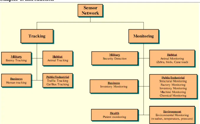
The wide varieties of user interest to real world make wide range of WSN applications. J. Yick classifies them into two categories: monitoring and tracking in (Yick, Mukherjee, & Ghosal, 2008). (see Figure 1-1). Monitoring applications include indoor/outdoor environmental monitoring, health and wellness monitoring, power monitoring, inventory location monitoring, factory and process automation, and seismic and structural monitoring. Tracking applications include tracking objects, animals, humans, and vehicles (Yick et al., 2008).
Chapter 1. Introduction
Figure 1-1 Overview of WSN applications(Yick et al., 2008)
Nowadays there are many WSN nodes such as BTnodes, l’ESB/2 nodes, SmartTags, EYES node, TinyNode, Mote, Mica2, Tmote Sky, Atlas and Imote (Akyildiz, Su, Sankarasubramaniam, & Cayirci, 2002; Baronti et al., 2007; Basaran et al., 2006; Yick et al., 2008) implemented to fulfill the huge amount of applications. Note that, all these WSN nodes are quite similar in term of functionality. They are based on 8 or 16-bit RISC microcontroller, such as Atmel AVR (Atmel-Corporation, 2012b), MSP430 (Texas-Instruments, 2012) etc., equipped with a unique Bluetooth or ZigBee wireless access medium having 200m LOS ‘Line Of Sight’ range (Basaran et al., 2006), and enable to implement a simple wireless sensor application. These WSN nodes have been designed with highly resource constraint, so the fault tolerant is not highly considered during the design process.
Notice that in real world applications, WSN nodes will be deployed in open harsh environment. They may suffer different faults such as physical damage, environmental hazards, interference etc. Therefore based on these faulty sensor nodes, researchers have developed many techniques to increase the reliability of the whole network. Redundant use of WSN nodes, reorganization of sensor network, and overlapped sensing regions are few of the techniques employed to increase the fault tolerance or reliability of the network (Gao, Xu, & Li, 2007; Hsieh, Leu, & Shih, 2010; Khan, Daachi, & Djouani, 2012; M.-H. Lee & Choi, 2008; Nakayama, Ansari, Jamalipour, & Kato, 2007).
This dissertation focuses on developing a reliable WSN from the early stage. We want to develop a more reliable WSN node comparing with the existing one. To achieve this goal, we will introduce a new design process to develop and implement WSN node. The reliability of Very Large Scale Integration (VLSI) is highly improved during recent decades. One of the
most important reasons for the success of VLSI technique is that the whole industry makes Design for Testability (DFT) as their industry standard. DFT makes it possible to assure the detection of all faults in a circuit, reduce the cost and time associated with test development, and reduce the execution time of performing test on fabricated chips.
Figure 1-2 shows the block diagram of a simple DFT system.
Design Under Verification
Source Check
Reference Model
Test Bench
Figure 1-2 Block diagram of DFT system
As we expect our WSN node to be more reliable, and DFT exactly meets this requirement. Therefore, our motivation is applied the DFT concept to our WSN design process in order to improve its reliability.
1.2.
Our Multicore Solutions
Figure 1-3 presents the block diagram of a multicore DFT solution for WSN. To transplant the DFT concept to a new WSN node, first we put the center microcontroller, application core, of tradition sensor node as Design under Verification (DUV) module. Then, we add another core to run the Test Bench (TB) module. We name this core as Fault Detect and Fault Recover Core (FD & FR Core). We use separate core to test and validate the application core in order to avoid the intra-system interference.
Chapter 1. Introduction Application Core Source Check Reference Model
FD&FR Core
Figure 1-3 Block diagram of Multicore WSN node
When faults show up in the application core, which is running the user application software, the FD & FR Core can detect and identify the faults, similarly as TB module do in module/chip validation process, then help the faulty node recover from these faults. The multicore WSN node can tolerate these faults automatically. Because the test and validation process in multicore WSN node is carried out in real-time, so we name this method as Design for Multicore Run Time Testability (DMRTT). Moreover, the application core in DUV module may have a redundancy for further improving reliability as shown in Figure 1-4.
Active Core
Source Check
Reference Model
FD&FR Core
Standby Core
Figure 1-4 Block diagram of Multicore WSN node with redundancy for application core It is known to all that the energy constrain of WSN node is very high. Normal microcontroller is too big in form factor and high in power consumption to be the FD & FR Core. Therefore, we introduce Nano Controller (NC) to be the FD & FR Core. NC is a very small and ultra-low power consumption controller. Because it is very small, so it will not notably affect the cost and complexity of WSN node. Moreover, it is an ultra-low power
consumption controller, which consumes only one percent energy of normal microcontroller, so it can help WSN node to be more energy efficient when the application core is switched off. DMRTT and NC together form our multicore architecture, which can greatly improve the reliability and energy efficiency of WSN node without significant increase in cost and complexity.
1.3.
Contributions
The contributions of this dissertation are in the area of fault tolerance, specifically in the field of system design and hardware platform design of fault tolerance WSN. Overall, the main contributions of this dissertation are:
We first present a novel modular multicore architecture that meets the strict dependability and energy efficiency requirements of wireless sensor networks. The multicore architecture can highly improve the reliability of WSN without sacrificing simplicity.
Then, we present a design process (High Reliability Design Process dedicated to Resource Constraint Embedded System: HRDP) based on multicore architecture to ease the development of dependable WSN. The HRDP can easily adjust to apply in any resource constrained embedded system to improve the reliability.
Finally, we demonstrate the flexibility of our multicore architecture on several hardware platforms, E²MWSN, iLive, SIS, iLiveEdge, EPER, RPiER, etc. These hardware platforms already form some WSN in different long-term, battery operated real-world applications. They can meet the application requirements very well.
1.4.
Dissertation Structure
This dissertation has seven chapters. The remainder of the dissertation is organized as follows:
Chapter 2, General Purpose Dependable System, presents a survey of dependable system. It tries to provide the necessary background for a general understanding of the issue discussed in later chapters.
Chapter 3, Dependable Wireless Sensor Networks, provides a general overview of the dependable WSN. By considering the needs of applications, this chapter describes the shortcomings of traditional wireless architectures and current approaches motivates design choices made later in this dissertation.
Chapter 4, Multicore WSN Node Architecture, presents the overall framework, multicore architecture, to address the dependability of WSN. The designing goal of our multicore
Chapter 1. Introduction
architecture is trying our best to improve the reliability of WSN without significant increasing cost and complexity.
Chapter 5, High Reliability Design Process dedicated to Resource Constraint Embedded System, discusses the design process (High Reliability Design Process dedicated to Resource Constraint Embedded System: HRDP) that developers may carry out to make full use of multicore architecture. The HRDP and multicore architecture are both technologies independent, they both can easily adjust to any resource constrained embedded system to improve the reliability.
In Chapter 6, Implementation of Multicore Wireless Sensor Node, we present several hardware platforms, E²MWSN, iLive, SIS, iLiveEdge, EPER, RPiER, etc., and several real-world applications based on these platforms. These hardware platforms will demonstrate the flexibility of our multicore architecture. Additionally the applications will validate the real-world performances of our architecture.
Chapter 7 summarizes the thesis and concludes with a prediction of future technological trends.
Chapter 2. General Purpose Dependable System
The dependability of computer system has been a challenge ever since computers first appeared in the middle of the 20th century. In those days, computers were built by using unreliable components such as vacuum tubes, relays, and so on. They were expensive, and used mainly by government and big corporations.
Nowadays, computers are built from more reliable components, such as semiconductor components, and other components from more advanced technology. With the ever-increasing circuit density, computers are more reliable and no longer expensive commodities thanks to fault detections and corrections techniques (Blundell, 2007). They becoming an every-day commodity, deeply embedded in practically every aspect of our lives, from visible desktops, laptops, smart phones etc., to invisible vital components of cars, home appliances, medical equipment, aircraft, industrial plants, and power generation and distribution systems.
As we are increasingly dependent on services provided by computer systems and our vulnerability to computer failures is also growing. We would like these systems to be dependable: they should still deliver an acceptable level of service in spite of faults. Notice that how to design a low cost robust embedded system is still a challenge.
In this chapter, we will present a survey of the techniques dedicated to dependable system. These techniques will be the fundamentals of our target fault tolerant wireless senor network.
2.1. Introduction
Dependability is defined in (A. Avizienis, Laprie, Randell, & Landwehr, 2004) as the ability to deliver service that can justifiably be trusted. It also encompasses mechanisms designed to increase and maintain the dependability of a system. Dependability covers the availability performance and its influencing factors: reliability performance, maintainability performance and maintenance support performance (including management of obsolescence). The International Electrotechnical Commission (IEC), via its Technical Committee TC 56 develops and maintains international standards in the field of dependability (IEC, 2013).
Before giving more details on different technical methods for improving dependability, we firstly discuss overview of dependability concepts.
Chapter 2.General Purpose Dependable System
Figure 2-1 The dependability tree (Algirdas Avizienis, Laprie, & Randell, 2001)
Figure 2-1 shows a systematic exposition of the concepts of dependability (Algirdas Avizienis et al., 2001), it can be broken down into three elements:
Attributes - A way to assess the dependability of a system;
Threats - An understanding of the things that can affect the dependability of a system; Means - Ways to increase a system's dependability;
Dependability is a generic concept that is led by three groups of fundamental concepts: its attributes, the threats to its attainment and the means to reach the desired dependability goals.
2.1.1.
Dependability Attributes
The dependability attributes represent different aspects of the service delivery. They are used to express and analyze the quality of the service delivered or expected from the system. Based on the needs of the user(s), several kinds of attributes can be found, but they are almost compositions or specializations of the following basic ones:
Availability (A(t)): The probability that a system is operating correctly and is available to perform its functions at the instant of time t.
Reliability (R(t)): The conditional probability that a system has functioned correctly throughout an interval of time, [t0, t], given that the system was performing correctly
at time t0.
Safety (S(t)): The probability that a system will either perform its functions correctly or will discontinue its functions in a well-defined, safe manner.
Confidentiality: absence of unauthorized disclosure of information Integrity: absence of improper system state alterations
Maintainability (M(t)): The probability that an inoperable system will be restored to an operational state within the time t.
2.1.2.
Dependability Threats
The threats to dependability are faults, errors and failures. They are the circumstances at the origin of an incorrect service delivery. Their effects deteriorate the level of satisfaction of the dependability attributes.
Fault: A physical defect, imperfection, or flaw that occurs in hardware or software; A fault is the adjudged or hypothesized cause of an error. A fault is active when it produces an error, otherwise it is dormant
Error: The occurrence of an incorrect value in some unit of information within a system; An error is that part of the system state that may cause a subsequent failure Failure: a deviation in the expected performance of a system; A failure occurs when
an error reaches the service interface and alters the service, i.e., system cannot provide correct system function.
2.1.3.
Dependability Means
The development of a dependable computing system calls for the combined utilization of a set of four techniques:
Fault prevention: A technique that an attempts to prevent the occurrence of faults; It is more related to general engineering processes and is handled by quality control techniques employed during design and development of systems.
Fault tolerance: The ability to continue the correct performance of functions in the present of faults; It is carried out via the implementation of error detection and system recovery mechanisms.
Chapter 2.General Purpose Dependable System
Fault removal: A technique that deals with how to reduce the number or severity of faults; It can be carried out both during the development phase, and during the use phase of a system. In development phase, it consists of verification, diagnosis and correction. In use phase, it consists in a corrective or a preventive maintenance. Fault forecasting: A technique that deals with how to estimate the present number,
the future incidence, and the likely consequences of faults. It is conducted by carrying out an evaluation of the system behavior with respect to fault occurrence or activation.
In order to improve the dependability, the combinations of those techniques are strongly recommended. In this dissertation, the architecture of our WSN node is directly support fault tolerance; we will use fault removal in the development phase to help verify each components and whole system; fault prevention is handled thought out all the design process.
2.2. Dependability Evaluation Techniques
As Peter Drucker once said: “If you can’t measure it, you can’t manage it.” (Brown, 1982) If we cannot estimate the dependability of present and the future candidate design, we cannot make good decisions. Therefore, we need use dependability evaluation techniques in design process to help to estimate the dependability of design, and then improve it.
2.2.1.
Dependability Terms
2.2.1.1. Failure rateA failure rate is the expected number of failures per unit time. For example, if a processor fails, on average, once every 1000 hours, then it has a failure rate failures/hour. (Dovich, 1990) (IEC, 2013)
The failure of a system is
1 N i i
(2.1)While iis the failure rate of sub system.
From failure rate , we can have Reliability (R(t)):
( ) t
R t e (2.2)
The common used unit of failure rate is FIT (Failures in Time Failure Rate in Parts per Billion Hours). One FIT equals one failure per billion (109) hours (once in about 114,155 years). The FIT is especially good for the failure rate of individual components, since their failure rates are often very low.
Figure 2-2 and Figure 2-3 provide a typical evolution of failure rate over a lifetime of a hardware system and a software system (Dubrova, 2013).
Figure 2-2 Typical evolution of failure rate over a lifetime of a hardware system (Dubrova, 2013)
Figure 2-3 Typical evolution of failure rate over a lifetime of a software system (Dubrova, 2013) As shown in Figure 2-2, hardware failures rate can typically characterize by a bathtub curve. The chance of a hardware failure is high during the initial life of the module (Phase I). The failure rate during the rated useful life (Phase II) of the product is low. Once the end of the life (Phase III) is reached, failure rate of modules increases again.
Software failures rate, however, does not show the same characteristics similar as hardware. A possible curve is shown in Figure 2-3 if we projected software failures rate on the same axes (Reliability Analysis Center, 1996). There are two major differences between hardware and software curves. One difference is that in the last phase (Phase III), software does not have an increasing failure rate as hardware does. In this phase, software is approaching obsolescence; there is no motivation for any upgrades or changes to the software. Therefore, the failure rate will not change. The second difference is that in the useful-life phase (Phase II), software will experience a drastic increase in failure rate each time an upgrade is made. The failure rate levels off gradually, partly because of the defects found and fixed after the upgrades.
Chapter 2.General Purpose Dependable System
2.2.1.2. Mean time to failure
Another important and frequently used measure of interest is mean time to failure defined as follows. The mean time to failure (MTTF) of a system is the expected time of the occurrence of the first system failure (Dubrova, 2013).
0 ( ) MTTF R t dt
(2.3) 0 0 1 1 [ ] t t MTTF e dt e
(2.4)2.2.1.3. Mean time to repair
The mean time to repair (MTTR) of a system is the average time required to repair the system. MTTR is commonly specified in terms of the repair rate μ, which is the expected number of repairs per unit time (Dubrova, 2013):
1
MTTR
(2.5)
From the definition of MTTF and MTTR, we can have Availability: 100% MTTF MTTF Availability MTTR (2.6)
2.2.1.4. Mean time between failures
The mean time between failures (MTBF) of a system is the average time between failures of the system. The MTBF should be used as part of a model that assumes the failed system will be repaired immediately (zero elapsed time) as opposed to mean time to failure (MTTF), which measures average time between failures of non-repairable systems only. However, in practice, MTBF is commonly used for both types of systems, repairable and non-repairable (Reliability Information Analysis Center, 2005; Zzyzx Peripherals, 2001).
MTBF is a measure of how reliable a hardware product or component is. It describes the flat, bottom of the bathtub curve of failure rate. MTBF is equal to the inverse of failure rate.
1
MTBF
(2.7)
Note that many products with very low failure rates during "normal life" will wear out in a few years, so that the Lifetime may be much less than MTBF. The Figure 2-4 shows the relationship between MTBF and Lifetime.
Figure 2-4 MTBF versus Lifetime
Unlike the hours from the MTBF calculations, lifetime indicates the operating hours expected under normal operating conditions. The lifetime is the period of time between starting to use the device and the beginning of the wear-out phase. This period of time is determined by the life expectancy of the components used in the assembly of the unit. As with any design, the weakest component with the shortest life expectancy determines what the life of the whole product will be. For example in power supplies, the electrolytic capacitors have the shortest lifetime expectancy.
So the lifetime is determined by the weakest component, so the redundancy cannot help to improve the lifetime. Meanwhile the MTBF can be highly affected by the architecture (redundancy e.g.). In case of Dual Modular Redundant (DMR) system with same component, each component has MTBF1000 hours, the MTBF of the DMR system is 1,000,000 hours. While in case of Triple Modular Redundant (TMR) system with same each component has MTBF1000 hours, the MTBF of the TMR system will increase to 1,000,000,000 hours. 2.2.1.5. Mean time between critical failures
The mean time between critical failures (MTBCF) of a system is the average time between critical failures of the system. MTBCF is a subset of MTBF because it only counts those failures that result in a mission abort or mission failure. The reliability analyst needs to be able to distinguish between those failures that are critical to the mission versus those that are not (failures that are not critical to the mission will still need to be fixed and counted as part of the MTBF calculation)(Reliability Information Analysis Center, 2005).
Chapter 2.General Purpose Dependable System
2.2.1.6. Summary
In this dissertation, we mainly use MTBF and MTBCF to evaluation the dependability of different WSN architecture. Therefore, we focus on the core and necessary external components, the rest components such as PCB board, connectors, sensors, batteries, RF antenna, etc. are not taken into account.
2.2.2.
Dependability model types
There are mainly two common dependability models: reliability block diagrams and Markov processes. Reliability block diagrams belong to a class of combinatorial models, which assume that the failures of the individual components are mutually independent. Markov processes belong to a class of stochastic processes, which take the dependencies between the component failures into account, making the analysis of more complex scenarios possible.
Combinatorial reliability models include reliability block diagrams, fault trees, success trees and reliability graphs. Figure 2-5 show an example of serial and parallel two-component system.
Figure 2-5 Reliability block diagram of a two-component system: (a) Serial, (b) parallel First, reliability block diagrams assume that the system components are limited to the operational and failed states and that the system configuration does not change during the mission. Hence, they cannot model standby components, repair, as well as complex fault detection and recovery mechanisms. Second, the failures of the individual components are assumed to be independent. Therefore, the case when the sequence of component failures affects system reliability cannot be adequately represented (Reliability Analysis Center, 1996).
Contrary to combinatorial models, Markov processes take into account the interactions of component failures making the analysis of complex scenarios possible.
The WSN node is only a tiny design, so in this dissertation, we chose reliability block diagrams as the dependability models of our design.
2.2.3.
Dependability computation methods
The computation methods of dependability are based on the model of dependability. Therefore, in this dissertation, we mainly discuss the computation methods based on Reliability block diagrams. Reliability block diagrams can be used to compute system reliability as well as system availability.
2.2.3.1. Reliability computation
To compute the reliability of a system represented by a reliability block diagram, we need first to break the system down into its serial and parallel parts. Next, the reliabilities of these parts are computed. Finally, the overall solution is composed from the reliabilities of the parts.
Given a system consisting of n components with R t being the reliability of the ii( ) th component. If the n components are serial parts, the reliability of the overall system is given by (Dubrova, 2013)
( )serial ni i( )
R t R t (2.8)
Else, if the n components are parallel parts, the reliability of the overall system is given by (Dubrova, 2013)
( ) 1 n(1 ( ))
parallel i i
R t R t (2.9)
For example, if a serial system with 100 components is to be built, and each of the components has a reliability 0.+999, the overall system reliability is 0.905.
In case of parallel system having 5 components, each component has a reliability 0.96, the reliability of the system is 0.999999.
2.2.3.2. Availability computation
If we assume that the failure and repair times are independent, then we can use reliability block diagrams to compute the system availability. This situation occurs when the system has enough spare resources to repair all the failed components simultaneously. Given a system consisting of n components with Ai(t) being the availability of the ith component, the
availability if the overall system is given by (Dubrova, 2013)
( )serial ni i( )
A t A t (2.10)
( )parallel 1 ni(1 i( ))
Chapter 2.General Purpose Dependable System
2.3. Fault Tolerance and
Redundancy
As be mentioned before, in order to improve the dependability, the combinations of different dependable means should be used in the development of WSN nodes. Beyond fault removal in the development phase and fault prevention in all the design process, the ability of fault tolerance of whole design should be most important feature. It is practically impossible to foresee all the factors and run the system in a perfect environment. So the system is requested to continue the correct performance of functions in the present of faults, support fault-tolerance. Therefore, in this part, we will intro various redundancy approaches to achieve fault-tolerance.
Redundancy is the provision of functional capabilities that would be unnecessary in a fault-free environment. There are mainly two kinds of redundancy: space and time. Space redundancy provides additional components, functions, or data items that are unnecessary for a fault-free operation. Space redundancy is further classified into hardware, software and information redundancy, depending on the type of redundant resources added to the system. In time redundancy, the computation or data transmission is repeated and the result is compared to a stored copy of the previous result (Dubrova, 2013).
2.3.1.
Space Redundancy
2.3.1.1. Hardware RedundancyHardware redundancy is achieved by providing two or more physical instances of a hardware component. For example, a system can include redundant processors, memories, buses or power supplies. Hardware redundancy is often the only available method for improving the dependability of a system, when other techniques, such as better components, design simplification, manufacturing quality control, software debugging, have been exhausted or shown to be more costly than redundancy.
There are three basic forms of hardware redundancy: passive, active and hybrid (Dubrova, 2013).
Passive redundancy achieves fault tolerance by masking the faults that occur without
requiring any action on the part of the system or an operator.
Active redundancy requires a fault to be detected before it can be tolerated. After the
detection of the fault, the actions of location, containment and recovery are performed to remove the faulty component from the system.
Hybrid redundancy combines passive and active approaches. It can mask the fault like in
passive redundancy and reconfigure to recovery like in active redundancy. It is more reliable but more expensive than previous methods.
2.3.1.2. Software Redundancy
Reliability in software domain is still an open issue; it is not as well understood as fault-tolerance in hardware domain. There are controversial opinions on whether reliability can be used to evaluate software. Software failures are mostly due to the activation of design faults by specific input sequences. This makes the reliability of a software module dependent on the environment that generates input to the module over the time.
Many current techniques for software fault tolerance are trying to follow the same schemes of hardware redundancy. They can be divided into two groups, single-version techniques and multi-version techniques (Dubrova, 2013).
Single version techniques aim to improve fault-tolerant capabilities of a single software module. It consists of fault detection, containment and recovery mechanisms. The recovery processes use the concept of retrying the same operation in expectation that the problem is resolved after the second try.
Multi-version techniques employ redundant software modules, developed following design diversity rules. The software version programming closely resembles hardware N-modular redundancy.
2.3.1.3. Information Redundancy
Information redundancy techniques add extra information to date to tolerate faults. They can be divided into two types: error detecting codes and error correcting codes (Wikipedia, 2013).
Error detection is the detection of errors caused by noise or other impairments during transmission from the transmitter to the receiver. Error detecting code is most commonly realized using a suitable hash function (or checksum algorithm). A hash function adds a fixed-length tag to a message, which enables receivers to verify the delivered message by recomputing the tag and comparing it with the one provided.
Error correction is the detection of errors and reconstruction of the original, error-free data. An error-correcting code (ECC) or forward error correction (FEC) code is a system of adding redundant data, or parity data, to a message, such that it can be recovered by a receiver even when a number of errors (up to the capability of the code being used) were introduced, either during the process of transmission, or on storage.
2.3.2.
Time Redundancy
Space redundancy techniques discussed so far impact physical entities like cost, weight, size, power consumption, etc. In some applications, extra time is of less importance than extra hardware, and then time redundancy will be a better solution. Time redundancy is achieved by
Chapter 2.General Purpose Dependable System
repeating the computation or data transmission and comparing the result to a stored copy of the previous result. If the repetition is done twice, and if the fault, which has occurred, is transient, then the stored copy will differ from the re-computed result, so the fault will be detected. If the repetition is done three or more times a fault can be corrected. Permanent faults can also be detected by repeating computation several times using different coding schemes.
Apart from detection and correction of faults, time redundancy is useful for distinguishing between transient and permanent faults. If the fault disappears after the re-computation, it is assumed to be transient. In this case, the hardware module is still usable and it would be a waste of resources to switch it off the operation. Otherwise, if the fault is permanent, the system of course should switch off or go to a safety state to avoid affect the rest parts of other system.
2.4. MTBF Values Evaluation
The MTBF value of COST component (microcontroller e.g.) is calculated from failure rate , which normally provided by manufacturer. The manufacturer (Atmel (Atmel-Corporation, 2012c) e.g.) provides the FIT data of component under optimal conditions and only related to hardware. According to Blue Max Technology, “Stressing a component beyond normal usage conditions may reduce the actual MTBF to a point below the ‘predicted MTBF’. Generally, reliability decreases as temperature increases, so components that are operated in warm environments with poor air flow will tend to have a lower MTBF than those operated in cool environments with good air flow.” According to Military & Aerospace Technology, “For every 10ºC you increase temperatures on electronics, your MTBF will be cut in half, so the hotter the electronics get, the lower the MTBF.” The temperature and the humility are not only part of the parameters, which will affect the reliability of our design. The reliability of system will also be affected by other parameters such as interference, metastability, high-energy particles, software bug, misuse of the hardware and SRAM transition fault (Autran et al., 2012). That is why the real experience of error free period is always much shorter than the theoretical MTBF provided by the manufacturer.
For example, the MTBF of a standard PC is 30,000 hours or 3.4 years (Minicom Advanced Systems Ltd., 2013). The MTBF estimates for the Intel® Server System is about 50,000 hours (Intel Corporation, 2013a). The Figure 2-6 shows the MTBF Estimates of sub and total system of Intel® Server System R1208RPMSHOR.
Figure 2-6 MTBF Estimates for Intel® Server System R1208RPMSHOR (Intel Corporation, 2013a) From the Figure 2-6, we can find that the most robust sub system of Intel® Server System R1208RPMSHOR is Front Panel board. Its MTBF is 8,272,282 hours, 944 years. The server board S1200V3RPM’s MTBF is 371,523 hours, 42 years. As mentioned in Figure 2-4, the MTBF/MTBCF is related to the failure rate (bottom of the bathtub curve) of the system, not the product lifetime. Therefore, we cannot say that Front Panel board can work for 944 years or server board S1200V3RPM can work for 42 years. Of course, from our own experience, we can easy to find out that server (with high MTBF) is normally more reliable than the PC (with low MTBF) and demands less reboot requirements. The MTBF trend is concurrent with our user experience.
Warranty firm Square Trade has released a research paper analyzing the failure rate for 30,000 laptops comparing brands and hardware categories in 2009 (SquareTrade, 2009). The headline news of the report is that over three years, one out of three laptops will fail, and that Asus and Toshiba laptops have the lowest failure rates, while Acer, Gateway, and HP have higher than average failure rates. Additionally, two-thirds of those problems are hardware malfunctions, while the final third are classified as accidental damage. The Figure 2-7 and the Figure 2-8 show the results in this report.
Chapter 2.General Purpose Dependable System
Figure 2-8 Three Years Laptop Malfunction Rates by Manufacturer (SquareTrade, 2009) From the Figure 2-7 and the Figure 2-8, we can know that the raw MTBF is concurrent with the malfunction rates of design in product life. However, everyone has the experience to reboot PC from time to time to fix some unknown problems. Those unknown problems make the one-time useable period of PC much short than the raw MTBF. The laptops normally work indoor with user-friendly interface for user to detect the running status and manually reboot to recovery from fault. This manually fault detection and recovery mechanical enable PC resume to work until it suffer malfunction.
Meanwhile, the WSN node is working in the outdoor environment, so even its raw MTBF is relative high, and the node will not suffer malfunction in short period, but without recovery mechanical, the one-time usable period will much shorter than the raw MTBF. In our experiments, the unicore WSN network will lose 20% of its nodes in only two-week time. Therefore, we proposed to use multicore architecture to enable to implement a WSN node, which supports fault auto detection and auto recovery. By using this new multicore WSN architecture, we want to improve greatly the usable period of WSN node. Furthermore, in some of multicore WSN instances, by adopted space redundancy, we will improve both the one-time usable period and the raw MTBF of WSN node at the same time.
2.5. RAS of Computer System
Reliability, availability, and serviceability (RAS) was originally introduced by IBM as a term to describe the robustness of their mainframe computers (International Business Machines Corporation, 1970). Different operational states of a IBM server based on RAS concepts are illustrated by the Figure 2-9 (IBM Corp, 2012). This combination of hardware and software self-recovery techniques are part of advanced RAS features that increase the availability of services that must be 24x7.
Figure 2-9 IBM server system RAS operations (IBM Corp, 2012)
For years, RAS already became a standard engineering term in computer system, especially in computer system of mission-critical applications such as database, enterprise resource planning (ERP), customer resource management (CRM), and business intelligence (BI) applications. These applications require being available 24x7 on a wide area or global basis. A failure affecting a single core business application can easily cost hundreds of thousands to millions of dollars per hour. In order to improve RAS, many approaches are adopted in different aspect of computer system. The IBM RAS server architecture is illustrated by the Figure 2-10. Moreover similar RAS system, non-stop servers, is also developed by HP (Hewlett-Packard Development Company, 2012).
Figure 2-10 Advanced RAS features of an IBM System x3850 X5 server (IBM Corp, 2012) The RAS architecture is symmetric space (processor, system bus, memory, devices and storage) and time redundancy (system recovery). The RAS concept used to implement very
Chapter 2.General Purpose Dependable System
expensive IBM and HP servers are not energy efficient. Due to the resource constraint, these approaches cannot directly use in WSN nodes. Thus, RAS concept cannot be applied to implement energy efficient multicore, modular WSN node.
2.6. Summary
In this chapter, we discussed the dependability concepts, dependability evaluation techniques, dependability terms, dependability model types, dependability computation methods, various redundancy approaches to achieve fault-tolerance, etc. Notice that, how to quantify the dependability of a real world system (HW and SW) is still an open question? The MTBF provided by the VLSI chip manufacturer is a quality indicator but it does not reflect the real world system MTBF.
In fact, a fault is a defect in hardware or software component. A manifestation of a fault, resulting in deviation from accuracy and faults may cause errors. A failure is a non-performance of expected action and errors may cause failures.
There are three types of fault: permanent, intermittent and transient. Intermittent faults occur because of unstable or marginal hardware due to environmental changes (loose connections, aging components, critical timing, interconnect coupling, resistive or capacitive variations and noise in the system). Transient faults occur because of high energy particles, temperature, humidity, pressure, voltage, power supply, vibrations, fluctuations, electromagnetic interference, ground loops, cosmic rays, alpha particles, cross talk, and electrostatic discharge. The error causes by non-permanent fault is a Soft Error ‘SE’. Permanent faults reflect irreversible physical changes. The improvement of semiconductor design and manufacturing techniques has significantly decreased the rate of occurrence of permanent faults (A. C. S. Beck, Lisbôa, & Carro, 2012).
Intermittent and transient faults are expected to represent the main source of errors experiences by VLSI circuits. Failure avoidance, based on design technologies and process technologies would not fully control intermittent and transient faults.
Fault tolerant solutions, presently employed in custom design systems will become widely used in off-the-shelf ICs (Mile Stojčev 2004). For the WSN outdoor application (harsh environment), there are many soft errors. Consequently for the wide spread use of outdoor WSN robustness is a main key feature.
In order to improve the dependability of our system, the following parts of this dissertation will mainly detail on fault tolerance architecture based on active redundancy, fault removal and fault prevention is the design process.
Chapter 3. Dependability
of
Wireless
Sensor
Networks
Unlike general-purpose computing systems, WSN nodes are not easily accessible for inspection and maintenance. At the same time, the nodes have far more stringent uptime requirements than general-purpose systems; 24/7/365 uptime is usually necessary. Moreover, WSN node has high resource constraint (limited power supply, memory and CPU) and some WSN nodes are working in mission critical applications. Therefore, these real world requirements demand a great deal of research in fault tolerance and dependable wireless sensor network. The following sections will discuss different WSN nodes, WSN application, dependability threats and current approaches. The shortages of current approaches motivate the need of multicore architecture presented in this dissertation.
3.1. Wireless Sensor Networks
3.1.1.
Introduction
Wireless Sensor Network ‘WSN’ is an active research field, which explores many technological challenges, while the WSN node design is one of the most challenging areas. The main constraints of WSN are resource and energy consumption. Consequently, the traditional embedded hardware and software solutions cannot be applied to WSN. For example, the Intel Itanium (9100 series features clock speed of up to 1.66 GHz and 667 MHz Front Side Bus (Intel Corporation, 2008)) consumes 104W. However, the energy content of a pair of alkaline AA 1.5V 2000mAh batteries is only 21.6kJ (2 * 1.5 * 2000 * 10-3 * 3600 = 2.16 *104 J). The power consumption of the WSN node is application dependent. It is relied on the sensor type, sample frequency, duty-cycling system, sleeping period, wireless access media, and so on. However, in order to achieve 5-years lifetime with a pair of alkaline batteries, the average power consumption must less than 137µW (2.16 *104 /3600/24/365/5 = 1.37*10-4 W). Furthermore, if takes into account discharge curve of the battery voltage, the average power consumption should be even less. Thus, a WSN node should fulfill a task as a PC but consume 1 million times less energy.
A wireless sensor network is composed of a set of WSN nodes deployed in a field of interest to monitor specific phenomena. The WSN nodes can be equipped with a variety of sensors, such as air temperature sensor, air humility sensor, light sensor, soil temperature
Chapter 3. Dependability of Wireless Sensor Networks
sensor and soil moisture sensor. These WSN nodes sense specific environment phenomena, perform simple signal processing, and then send data to a central server through sink node.
WSNs can be used for a wide variety of applications dealing with monitoring (precision agriculture, environment data collection, etc.), control (disturbed sensing and controlling), and surveillance (smart care, battle-fields surveillance, etc.).
The following part will briefly introduce currently existed WSN nodes and WSN Applications.
3.1.2.
WSN Nodes
Recent advances in Very Large Scale Integration (VLSI) chip designs, wireless network and Micro-Electro-Mechanical Systems (MEMS) have led to the development of low-cost, low-power, and small size WSN nodes. Different institutes or companies have developed various kinds of WSN nodes. An exhaustive survey on WSN hardware has been done by Tatiana Bokareva (Bokareva, 2013). The information on various sensors, WSN nodes, processor, radio chipsets, sensor network operating system, protocols is available at Sensor Network Museum (TIK WSN Research Group, 2013). Here we briefly introduce two types of WSN nodes: Scalar WSN nodes and Multimedia WSN nodes.
3.1.2.1. Scalar WSN Nodes
The common available Scalar WSN nodes include: MICAz
The processor board of MICAz is MPR2400, which is based on Atmel ATmega128L. The MICAz (MPR2400) IEEE 802.15.4 radio (ZigBee compliant) offers both high speed (250 kbps) and hardware network security (AES-128). Direct sequence spread spectrum radio provides resistance to RF interference and data security. The 51-pin expansion connector supports Analog Inputs, Digital I/O, I²C, SPI and UART interfaces. It provides 75-100 meter of outdoor range line of sight communication (1/2 wave dipole antenna).
MICA2
The processor and radio board used in MICA2 is MPR400, which is based on Atmel ATmega128L. The radio uses 868/916 MHz frequency band and supports data rate of 38.4kbps. A variety of sensors and data acquisition boards for the MICA2 mote is available which can be connected to the standard 51 pins expansion connector. Apart from its basic function as WSN node, it can also function as a base station when interfaced with MIB 510/MIB 520. The MIB510/MIB520 provides a serial/USB interface for both programming and data communications. Theoretically, it supports 150 meter of outdoor range for line of sight communication (1/4 wave dipole antenna).
Figure 3-2 Circuit Board of MICA2 Telos B
The MICA2 and MICAz motes are found to be more suitable for field deployment purposes. The Telos B motes have programming and data collection facility via USB and is thus suitable for testbed deployment in lab for experimentation. It utilizes IEEE 802.15.4/ZigBee compliant radio (2.4-2.4835 GHz) which enables 250kbps of data transfer. The Telos B is based on 8 MHz TI MSP430 microcontroller with 10kB RAM. It has 1MB external flash for data logging, integrated onboard antenna and optional sensor suite including integrated light, temperature and humidity sensor.