HAL Id: hal-00748951
https://hal.archives-ouvertes.fr/hal-00748951
Submitted on 6 Nov 2012
HAL is a multi-disciplinary open access
archive for the deposit and dissemination of
sci-entific research documents, whether they are
pub-lished or not. The documents may come from
teaching and research institutions in France or
abroad, or from public or private research centers.
L’archive ouverte pluridisciplinaire HAL, est
destinée au dépôt et à la diffusion de documents
scientifiques de niveau recherche, publiés ou non,
émanant des établissements d’enseignement et de
recherche français ou étrangers, des laboratoires
publics ou privés.
An adaptive test for zero mean
Cécile Durot, Yves Rozenholc
To cite this version:
Cécile Durot, Yves Rozenholc. An adaptive test for zero mean. Mathematical Methods of Statistics,
Allerton Press, Springer (link), 2006, 15 (1), pp.26-60. �hal-00748951�
M A T H E M A T I C A L M E T H O D S O F S T A T I S T I C S
AN ADAPTIVE TEST FOR ZERO MEAN C. Durot1 and Y. Rozenholc2
1Laboratoire de Math´ematiques, Universit´e Paris Sud 91405 Orsay cedex, France
E-mail: cecile.durot@math.u-psud.fr 2MAP5 – UMR CNRS 8145 – Universit´e Paris 5 45, rue des Saints-P`eres, 75270 Paris cedex 06, France
E-mail: yves.rozenholc@math-info.univ-paris5.fr
Assume we observe a random vector y ofRn
and write y = f + ε, where f is the expectation of yand ε is an unobservable centered random vector. The aim of this paper is to build a new test for the null hypothesis that f = 0 under as few assumptions as possible on f and ε. The proposed test is nonparametric (no prior assumption on f is needed) and nonasymptotic. It has the prescribed level α under the only assumption that the components of ε are mutually independent, almost surely different from zero and with symmetric distribution. Its power is described in a general setting and also in the regression setting, where fi= F (xi) for an unknown regression function F and fixed design points xi∈[0, 1]. The test is shown to be adaptive with respect to H¨olderian smoothness in the regression setting under mild assumptions on ε. In particular, we prove adaptive properties when the εi’s are not assumed Gaussian nor identically distributed.
Key words: adaptive test, minimax hypothesis testing, nonparametric alternatives, sym-metrization, heteroscedasticity.
2000 Mathematics Subject Classification: 62G10, 62G08.
1. Introduction
Assume we observe a random vector y ∈ Rn and write y = f + ε, where f is
the unknown expectation of y and ε = (ε1, . . . , εn)T is an unobservable random
vector with mean zero. Assume the εi’s are mutually independent with symmetric
distribution (we mean that for every i, εi has the same distribution as −εi). Our
aim is to build a nonasymptotic test for the null hypothesis H0: f = 0 against the
nonparametric composite alternative H1: f 6= 0, when no prior assumption is made
on f and as few as possible assumptions are made on ε. In particular, we do not
c
°2006 by Allerton Press, Inc. Authorization to photocopy individual items for internal or personal use, or the internal or personal use of specific clients, is granted by Allerton Press, Inc. for libraries and other users registered with the Copyright Clearance Center (CCC) Transactional Reporting Service, provided that the base fee of $50.00 per copy is paid directly to CCC, 222 Rosewood Drive, Danvers, MA 01923.
assume a priori that f belongs to a given smoothness class, and the εi’s are not
assumed identically distributed nor Gaussian. The proposed test is defined as a multi-test and is based on a symmetrization principle that exploits the symmetry assumption.
The problem of hypothesis testing in the general model y = f + ε has rarely been addressed in the literature. Baraud et al. (2003) consider the problem of testing the null hypothesis that f belongs to a given linear subspace of Rn. No
prior information on f is required, but they assume that the components of ε are independent with the same Gaussian distribution. Under the same assumptions, Baraud et al. (2005) propose a test for the null hypothesis that f belongs to a given convex subset of Rn.
An interesting particular case of the general model above is the regression model, which is obtained in the case where fi = F (xi) for all i = 1, . . . , n. Here, the xi’s
are nonrandom design points and F is an unknown function. In this context, many tests have been proposed for the null hypothesis that F belongs to a given set F against a nonparametric alternative. Typically, F is a parametric set of functions orF is restricted to a single function, which amounts to F = {0}. These tests are often based on a distance between a nonparametric estimator for F and an estimator for F that is computed under the null hypothesis, see, e.g., M¨uller (1992). This requires the choice of a smoothing parameter such as a bandwidth. Other tests consider the smoothing parameter itself as a test statistic, see, e.g., Eubank and Hart (1992). Another approach consists in building a test statistic as a function of estimators for the Fourier coefficients of F , see, e.g., Chen (1994). We refer to the book of Hart (1997) for a review of these methods.
Recently, the problem of adaptive minimax testing has been addressed. Suppose that the null hypothesis is F ≡ 0 and consider the alternative that F is bounded away from zero in the L2-norm,kF k2≥ ρ(n), and possesses smoothness properties.
The minimal rate of testing (that is the minimal distance ρ(n) for which testing with prescribed error probabilities is still possible) has been first derived in a white noise model with signal F . The result depends heavily on the kind of smooth-ness imposed, see Ingster (1982, 1993) and Ermakov (1991) for Sobolev smoothsmooth-ness and Lepski and Spokoiny (1999) for Besov smoothness. The optimal rate and the structure of optimal tests depend on the smoothness parameters, whereas these pa-rameters are usually unknown in practical applications. In the white noise model, Spokoiny (1996) proves that the minimal rate of testing for H0: F ≡ 0 is altered
by a log log n factor when F belongs to a Besov functional class with unknown parameters. He builds a rate optimal adaptive test based on wavelets. Gayraud and Pouet (2005) obtain similar results in a regression model for a composite null hypothesis under H¨olderian smoothness. They prove that, in the Gaussian model, the optimal rate of testing is altered by a log log n factor if the smoothness param-eter is unknown. They build an adaptive test which achieves the optimal rate over a class of H¨olderian functions with smoothness parameter s > 1/4 in a possibly non-Gaussian model. Other examples of adaptive tests are given by Baraud et al. (2003), H¨ardle and Kneip (1999) and by Horowitz and Spokoiny (2001). All these adaptive tests are defined as multi-tests. Roughly speaking, the authors first build a test Ts that is minimax for a fixed smoothness parameter s and reject the null
Most of non-adaptive tests for zero mean involve a smoothing parameter which is chosen in a somewhat arbitrary way (Staniswalis and Severini, 1991). Adaptive tests do not show this drawback but either they require the errors to be i.i.d. Gaussian (H¨ardle and Kneip, 1999, Baraud et al., 2003) or they are asymptotic (Horowitz and Spokoiny, 2001, Gayraud and Pouet, 2005). Moreover, existing tests involve estimation of the unknown variance. This requires either homoscedasticity (Gayraud and Pouet, 2005) or regularity assumptions on the variance (Horowitz and Spokoiny, 2001). On the contrary, our test requires very mild assumptions on the errors, is nonasymptotic and needs neither variance estimation nor arbitrary choice of a parameter. It has the prescribed level under the only assumption that the εi’s are mutually independent with symmetric distributions (the εi’s may have
different distributions). Moreover, it achieves the optimal rate of testing over the class of H¨olderian functions with smoothness parameter s > 1/4 in the case where the εi’s satisfy a Bernstein-type condition, and in particular, in the homoscedastic
Gaussian case. The test still achieves the optimal rate of testing for s≥ 1/4 + 1/p in the case where the εi’s possess bounded moments of order 2p for some p≥ 2.
The paper is organized as follows. The testing procedure is described in Sec-tion 2. It is also stated in this secSec-tion that the proposed test has the prescribed nonasymptotic level. In Section 3, we discuss implementation of the test. The power is studied in Section 4 under various assumptions on the εi’s. In Section 5,
we compute the rate of testing of the test in a regression model under a H¨olderian assumption. A simulation study is reported in Section 6 and the proofs are given in Section 7.
2. The Testing Procedure
Assume we observe a random vector y of Rn and write
y = f + ε,
where f is an unknown vector of Rn and ε is an unobservable random vector
with mean zero. Assume that the components of ε are independent and possess a symmetric distribution around zero, which means that for all i, εiand−εi have the
same distribution. Assume furthermore that for all i, εi is almost surely different
from zero. Our aim is to build a test with nonasymptotic level α for the hypothesis H0: f = 0 against H1: f 6= 0. Here, α is a fixed number in (0, 1). The test
is based on a symmetrization principle that exploits the symmetry assumption. Before describing the test more precisely, let us introduce some notation.
Notation:
• For every set A, let |A| denote the cardinality of A and let 1Abe the indicator
function of A, which means that 1A(x) equals 1 if x∈ A and 0 otherwise.
• Let w be a random vector of Rn, independent of y, with independent
compo-nents wi distributed as random signs: P (wi= 1) = P (wi=−1) = 1/2.
• For all u, v ∈ Rn, let u
× v be the vector of Rn with ith component (u
× v)i=
uivi.
• Let k · kn be the Euclidean norm in Rn.
• For every partition m of {1, . . . , n} into Dmnonempty subsets em,1, . . . , em,Dm,
Πm be the orthogonal projector onto the linear span of {tm,1, . . . , tm,Dm}. Thus
for all u∈ Rn and i = 1, . . . , n
(Πmu)i = Dm X j=1 µ 1 |em,j| X k∈em,j uk ¶ 1em,j(i), kΠmuk 2 n= Dm X j=1 1 |em,j| µ X k∈em,j uk ¶2 .
The test is based on the following heuristics. Under H0, y has the same
distribu-tion as w×y. Hence for every partition m of {1, . . . , n}, kΠmyk2nandkΠm(w×y)k2n
have the same distribution. Under H1, as f 6= 0, consider an (unobservable)
par-tition m such that for every e ∈ m the numbers (fi)i∈e all have the same sign.
Then for every e∈ m, |Pi∈efi| ≥ |Pi∈ewifi| with a strict inequality if wi =−1
and fi 6= 0 for some i ∈ e, hence one has kΠmfk2n > kΠm(w× f)k2n provided
wi =−1 and fi 6= 0 for some i ∈ {1, . . . , n}. Thus under H1 there exists m such
that kΠmyk2n tends to be larger thankΠm(w× y)k2n, whereas under H0,kΠmyk2n
andkΠm(w× y)k2n are of the same order of magnitude for every m. Therefore, we
propose to reject H0 if there exists m such thatkΠmyk2n exceeds a given quantile
ofkΠm(w× y)k2n. Since the quantiles ofkΠm(w× y)k2n cannot be computed (they
depend on the unknown distribution of y) we consider conditional quantiles given y. The precise construction of the test is as follows. Consider a collection of par-titionsM and positive numbers αm withPm∈Mαm= α. We reject H0 if there
exists m∈ M such that kΠmyk2nexceeds the y-conditional quantile ofkΠm(w×y)k2n
defined by
qmy(αm) = inf©x∈ R, P£kΠm(w× y)k2n > x| y
¤
≤ αmª.
The critical region of our test is thus
(1) sup
m∈M
©
kΠmyk2n− qmy(αm)ª> 0.
Note that qy
m(αm) can theoretically be computed since it only depends on the
known distribution of w, but its exact calculus requires about 2n computations
which cannot be performed in practice. Hence we estimate it through Monte-Carlo simulations, see Section 3. It is stated in the following theorem that the test has a nonasymptotic level α.
Theorem 1. Assume we observe y = f + ε, where f ∈ Rn and the ε i’s are
independent random variables with symmetric distribution. AssumeP (εi= 0) = 0
for all i = 1, . . . , n. Let M be a collection of partitions of {1, . . . , n}, let α and (αm)m∈Mbe positive numbers such thatα =Pm∈Mαm. Then
PH0 ¡ sup m∈M{ kΠm yk2n− qym(αm)} > 0¢≤ α. Remarks.
• Like the adaptive tests mentioned in the introduction, our test is a multi-test: the null hypothesis is rejected if one of the tests with critical regions{kΠmyk2n >
qy
m(αm)} rejects. A given partition m allows us to detect alternatives with a given
smoothness s, and adaptive properties arise from the use of many partitions. • Our method allows us to test the more general null hypothesis H0: f ∈ V ,
where V is a linear subspace of Rn, but for this problem, we need the ε
i’s to be
i.i.d. Gaussian. Let V be a linear subspace of Rn with dimension k < n, let Π
be the orthogonal projector onto V⊥ and let ∆ be the diagonal matrix of which
(n− k) first diagonal components equal 1 and the others are zero. There exists an orthogonal matrix O with Π = OT∆O. Now, let y
V be the random vector that
consists of the (n− k) first components of ∆Oy = OΠy, let fV be the expectation
of yV and let εV = yV − fV. If the εi’s are i.i.d. Gaussian, so are the components of
εV. Since testing f ∈ V amounts to testing fV = 0 within the model yV = fV+ εV,
this may be done by applying our method. Then the theoretical results we obtain in the i.i.d. Gaussian model for H0: f = 0 (see Sections 4 and 5) can be generalized
to H0: f ∈ V . We do not detail these results.
3. Practical Implementation By definition, qy
m(αm) is the 1− αm quantile of the discrete distribution with
support ©kΠm(u× y)k2, u∈ {−1, 1}nª, which puts mass k2−n at a given point x
of the above set if there exist k vectors u∈ {−1, 1}n withkΠ
m(u× y)k2= x. The
exact calculation of qy
m(αm) thus requires about 2n computations, which cannot
be performed in practice. We thus suggest estimation of this quantile instead of computing its exact value. The practical implementation of the test then is as follows. Draw independent random vectors w1, . . . , wB which all are distributed
like w and are independent of y. For every m∈ M, compute the empirical quantile defined by b qmB(αm) = inf n x∈ R, B1 B X b=1 1kΠm(wb×y)k2 n>x≤ αm o and reject H0if (2) sup m∈M © kΠmyk2n− bqmB(αm)ª> 0.
It is stated in the following theorem that the test with critical region (2) has asymptotically level α if B→ ∞. Therefore, it suffices to choose B large enough so that the level of this test is close to α. But our aim is to consider quite moderate B so we also provide in Theorem 2 a control of the level in terms of α and B, under the additional assumption that the distributions of the εi’s are continuous. This
result provides a control of what we lose in terms of first kind error probability when we consider the critical region (2) instead of (1).
Theorem 2. Under the assumptions of Theorem1, lim B→∞PH0 ¡ sup m∈M{kΠm yk2n− bqmB(αm)} > 0¢≤ α.
If moreover the distributions of the εi’s are continuous, then
PH0 ¡ sup m∈M{kΠm yk2 n− bqmB(αm)} > 0¢≤ α + X m∈M 2Dm−n+|M| √π 2√2B.
By Theorem 2, it suffices to choose B = c|M|2 with a large enough c > 0
so that the level is close to α. The estimation of qy
m(αm) then requires about
n|M|2computations. In practical applications, one can consider, for instance, the
collection of dyadic partitions Md defined in Section 5. The cardinality of Md is
about log2n hence, using B with order of magnitude (log2n)2, we get a level close
to the nominal level α in about n(log2n)2 computations.
The following theorem describes what we lose in terms of second kind error probability when we consider the critical region (2) instead of (1).
Theorem 3. For every m ∈ M, let δm < αm. Under the assumptions of
Theorem1, we have for every f∈ Rn
lim B→∞Pf ¡ sup m∈M{kΠ myk2n− bqBm(αm)} > 0¢≥ Pf¡ sup m∈M{kΠ myk2n− qym(δm)} > 0¢. 4. Power
In this section, we study the power of the test with critical region (1). By Theorem 3, similar results hold for the test with critical region (2) provided B is large enough. LetM be a collection of partitions of {1, . . . , n}. Let α and β be fixed numbers in (0, 1). Let (αm)m∈M be positive numbers such that α =Pm∈Mαm.
The aim of this section is to describe a subsetFn(β) of Rn\ {0} over which the
power of the test is greater than 1− β, i.e., which satisfies (3) Pf¡ sup
m∈M{kΠmyk 2
n− qmy(αm)} > 0¢≥ 1 − β, for all f ∈ Fn(β).
For every partition m, the subsets e∈ m which contain only one point do not contribute to the power of the test since their contributions to the norms of Πmy
and Πm(w× y) are identical. Hence we restrict ourselves to collections M which
do not contain what we call the trivial partition, that is the partition made up of n singletons. For every m∈ M, we set
Jm,1={j ∈ {1, . . . , Dm}, |em,j| = 1}, Jm,2={j ∈ {1, . . . , Dm}, |em,j| ≥ 2}
(hence Jm,26= ∅) and
Im= min j∈Jm,2|e
m,j|.
We study the power of the test under two different assumptions on the εi’s
integrability. First, we assume that the εi’s satisfy the following Bernstein-type
condition: there exist positive real numbers γ and µ such that for all integers p≥ 1,
(4) max
1≤i≤nE(ε 2p
i )≤ γp!µp−2.
Thus the εi’s possess bounded moments of any order and ε2i possesses an exponential
moment, hence the errors are much integrable. Note however that this assumption is less restrictive than the Gaussian assumption: if the εi’s are Gaussian with
bounded variance σ2
i ≤ σ2, then E(ε 2p
i )≤ p!(2σ2)p, so (4) holds with µ = 2σ2 and
γ = µ2. It is also less restrictive than the boundedness assumption: if
|εi| ≤ c for
all i, then (4) holds with µ = c2 and γ = µ2. Secondly, we assume there exist p
≥ 2 and µ > 0 such that
(5) max
1≤i≤nE(ε 2p i )≤ µp.
Note that under both assumptions, the εi’s possess bounded variances and fourth
moments: E(ε2
i)≤ σ2 and E(ε4i)≤ µ4 for all i and some positive σ and µ4. It is
also assumed in the sequel that|fi| ≤ L for all i = 1, . . . , n and a possibly unknown
L > 0.
4.1. Power under the Bernstein-type condition.
Theorem 4. Assume we observe y = f + ε, where the εi’s are independent
variables with symmetric distribution. Assume P (εi = 0) = 0 and |fi| ≤ L for
a positive number L and all i. Assume moreover (4) holds for all integers p≥ 1 and some positive γ and µ. Let M be a collection of partitions which does not contain the trivial one. Let α, β in (0, 1) and (αm)m∈M be positive numbers with
P
m∈Mαm= α. For every A = (A1, . . . , A5)∈ (0, ∞)5,m∈ M and f ∈ Rn let
∆1(m, f, A) = A1kf − Πmfk2n+ A2 s γDm β (6) + A3(√γ + µ + L2) · 1 + 1 Im log µ2D m β ¶¸ log µ 2 βαm ¶ + A4(√γ + µ + L2) s Dm · 1 + 1 Imlog µ2D m β ¶¸ log µ 2 βαm ¶ + A5L2|Jm,1|.
Then there exists an absolute A such that (3) holds with Fn(β) = n f ∈ Rn, kfk2n≥ inf m∈M∆1(m, f, A) o .
Hence our test is powerful over Fn(β) provided the constants A1, . . . , A5 are
large enough. This set is large if there exists m∈ M such that Πmf is close to f ,
Dm and|Jm,1| are small, while Imis large enough.
This result applies to the i.i.d. Gaussian model. Assume that the εi’s are i.i.d.
N (0, σ2) and in order to make appear the signal to noise ratio, assume that there
exists L > 0 such that |fi| ≤ σL for all i. Then (4) holds with µ = 2σ2 and
γ = µ2. Theorem 4 consequently applies with √γ and √γ + µ + L2 replaced by σ2
and σ2(1 + L2) respectively. However (see Section 7.7), one can obtain a slightly
sharper result by using Cochran’s theorem: the power of the test is greater than 1− β as soon as (7) kfk2n≥ inf m∈M ½ A1kf − Πmfk2n + A3σ2(1 + L2) · 1 + 1 Im log µ 2Dm β ¶¸ log µ 2 βαm ¶ + A4σ2(1 + L2) s Dm · 1 + 1 Im log µ2D m β ¶¸ log µ 2 βαm ¶ + A5σ2L2|Jm,1| ¾
for large enough Ak’s. This condition reduces to (8) kfk2n≥ inf m∈M ½ C1kf − Πmfk2n+ C2σ2 · log µ 2 βαm ¶ + s Dmlog µ 2 αmβ ¶¸¾ , where C1is an absolute constant and C2only depends on L, provided this infimum
is achieved at a partition m∗ ∈ M with (9) 1 Im∗ log µ2D m∗ β ¶ ≤ 1 and, e.g., |Jm∗,1| ≤ p Dm∗.
Instead of (9), Baraud et al. (2003) assume that (Dm+log(1/α))/(n−Dm) remains
bounded to prove that the power of their test is greater than 1− β under condi-tion (8). Hence, both tests are powerful on similar sets. However, unlike the test of Baraud et al. our test requires neither Gaussian nor homoscedasticity assumptions.
4.2. Power under the bounded moments assumption.
Theorem 5. Assume we observe y = f + ε, where the εi’s are independent
variables with symmetric distribution. Assume P (εi = 0) = 0 and |fi| ≤ L for a
positive numberL and all i. Assume moreover (5) holds for some p≥ 2 and µ > 0. Let M be a collection of partitions which does not contain the trivial one. Let α, β in (0, 1) and (αm)m∈M be positive numbers with Pm∈Mαm = α. For every
A = (A1, . . . , A6)∈ (0, ∞)6,m∈ M, and f ∈ Rn let ∆2(m, f, A) = A1kf − Πmfk2n+ A2(µ + L2) s Dm β (10) + A3p(µ + L2) · 1 + √1 Im µ Dm β ¶1/p¸ log µ 2 αm ¶ + A4(µ + L2) s pDm · 1 + √1 Im µD m β ¶1/p¸ log µ 2 αm ¶ + A5L2|Jm,1| + A6 µ β. Then there exists an absolute A such that (3) holds with
Fn(β) = n f ∈ Rn, kfk2 n≥ inf m∈M∆2(m, f, A) o .
Let us compare this with Theorem 4. There are two main differences between ∆1 and ∆2. First, the absolute constants A3 and A4 in ∆1 are replaced in ∆2 by
A3p and A4√p respectively. Next, the term
1 Im log µ 2Dm β 
in ∆1 is replaced in ∆2 by the greater term
1 √I m µD m β ¶1/p ,
which depends on the error integrability. Hence, as expected, the set where our test is powerful is larger under the Bernstein-type condition than under the bounded moments condition.
5. Rate of Testing In this section we assume
fi= F (xi), i = 1, . . . , n,
for fixed numbers xi∈ [0, 1] and an unknown F : [0, 1] → R. We aim at testing
H′
0: F ≡ 0 against H1′ : F 6≡ 0.
For this task, we consider the so-called collection of dyadic partitionsMd ={mk,
k∈ I}, where
I = {2l, l
∈ N, 2l
≤ n/2} and mk consists of the nonempty sets among
½ i, xi ∈ µj − 1 k , j k ¸¾ , j = 1, . . . , k.
Let α and β in (0, 1) and αm= α/|Md|. As in Section 4, we restrict our attention
to the test with critical region (1), which still has level α in this setting. The aim of this section is to study the power of this test when the εi’s satisfy either (4) or (5)
and F is assumed H¨olderian. In particular, we aim at proving adaptive properties of the test with respect to H¨olderian smoothness. We distinguish between the cases where the H¨olderian smoothness of F is at most one or greater than one.
Assume the H¨olderian smoothness of F to be at most one: there exist s∈ (0, 1], R > 0, and L > 0 such that
(11) ∀(u, v) ∈ [0, 1]2,
|F (u) − F (v)| ≤ R|u − v|s, and sup
u∈[0,1]|F (u)| ≤ L. Assume moreover (12) |Jmk,1| ≤ a0 p Dmk and Imk≥ an k , all k∈ I,
for absolute constants a0 ≥ 0 and a > 0. This means that the design points are
almost equidistant. In particular, the condition is satisfied with a0= 0 and a = 1/2
if xi= i/n for all i. The following corollary of Theorems 4 and 5 provides conditions
on f under which the test is powerful, that is (13) Pf¡ sup
m∈M{kΠ
myk2n− qmy(αm)} > 0¢≥ 1 − β.
For the sake of simplicity, it is assumed that αm= α/|Md| for every m but it is
worth noticing that the results remain true ifPm∈Mαm= α and αm≥ (log2n)−cα
Corollary 1. Assume we observe y = f + ε, where the εi’s are independent
variables with symmetric distribution and fi = F (xi) for fixed xi ∈ [0, 1] and an
unknownF . Assume P (εi= 0) = 0 for all i and F satisfies (11) for unknown s∈
(0, 1], R > 0, and L > 0. LetM = Md be the collection of dyadic partitions. Let
α and β in (0, 1). For every m∈ M, let αm= α/|M|. Assume furthermore (12).
1. If (4) holds for all integers p≥ 1 and some positive numbers γ and µ, then (13) holds whenevern is large enough and one of the three following conditions is fulfilled for a large enough C (here, δ = √γ + µ + L2 andC only depends on a, a
0,α, β): (a) s > 1/4 and √1 nkfkn≥ CR 1/(1+4s) µδ√log log n n ¶2s/(1+4s) ; (b) s = 1/4 and √1nkfkn≥ CR2/3n−1/4δ1/6(log n× log log n)1/12;
(c) s < 1/4 and √1nkfkn≥ CRn−s.
2. If (5) holds for some p≥ 2 and µ > 0, then (13) holds whenever n is large enough and one of the three following conditions is fulfilled for a large enough C (here, δp= √p(µ + L2) and C only depends on a, a0,α, β):
(a) s≥ 1/4 + 1/p and √1nkfkn≥ CR1/(1+4s) µ δp√log log n n ¶2s/(1+4s) ; (b) s∈ [1/4 − 1/p, 1/4 + 1/p) and 1 √nkfkn≥ CR(2+3p)/(2+3p+8ps) µ δp√log log n n5/4 ¶4ps/(2+3p+8ps) ; (c) s≤ 1/4 − 1/p and √1nkfkn≥ CRn−s.
If xi = i/n for all i and F satisfies (11) then
1
√nkfkn ≥ kF k2− Rn−s.
Hence in that case, Corollary 1 holds withkfkn/√n replaced by kF k2. In
partic-ular, if s > 1/4 and (4) holds with µ = 2σ2and γ = µ2(which is indeed the case if
the εi’s are i.i.d.N (0, σ2)), then the power of the test is greater than a prescribed
1− β whenever n is large enough and kF k2≥ CR1/(1+4s)
µ
σ2√log log n
n
¶2s/(1+4s)
for a positive C, which only depends on L/σ, α, and β. This rate is precisely the minimal rate of testing obtained by Spokoiny (1996) in a white noise model. It is also the minimal rate of testing obtained by Gayraud and Pouet (2005) in the i.i.d. Gaussian regression model (but they do not describe the role of R and σ in this setting). This proves that our test achieves the optimal rate of testing under the
Bernstein-type condition (4) if s > 1/4, and also under the less restrictive moment condition (5) if s ≥ 1/4 + 1/p. In the case where s ≤ 1/4, the optimal rate of testing is not known, even in the i.i.d. Gaussian model. Note however that the rate Rn−s (obtained when s < 1/4 and (4) holds, and also when s
≤ p − 1/4 and (5) holds) was already obtained by Baraud et al. (2003) in the i.i.d. Gaussian setting for s < 1/4.
Now, assume the H¨olderian smoothness of F to be greater than one: there exist d∈ N \ {0}, κ ∈ (0, 1], R, and L such that
(14) ∀(u, v) ∈ [0, 1]2, |F(d)(u)− F(d)(v)| ≤ R|u − v|κ, and sup
u∈[0,1]|F (u)| ≤ L.
Here, F(d) denotes the dth derivative of F (which is assumed to exist) and we
denote by s = d + κ the H¨olderian smoothness of F . For technical reasons, we restrict ourselves to the case where xi= i/n for all i.
Corollary 2. Assume we observe y = f + ε, where the εi’s are independent
variables with symmetric distribution andfi= F (i/n) for an unknown F . Assume
P (εi = 0) = 0 for all i and F satisfies (14) for unknown d ∈ N \ {0}, κ ∈ (0, 1],
R > 0, and L > 0. Let s = d + κ > 1 and letM = Md be the collection of dyadic
partitions. Let α and β in (0, 1). For every m ∈ M, let αm = α/|M|. Assume
furthermore that either(4) holds for all integers p≥ 1 and some positive numbers γ and µ, or (5) holds for some p≥ 2 and µ > 0. Then there exists C > 0, which only depends on α, β, and s, such that (13) holds whenever n is large enough and
(15) kF k2≥ CR1/(1+4s) µ δ√log log n n ¶2s/(1+4s) .
Here, δ = √γ + µ + L under assumption (4) and δ = √p(µ + L2) under
assump-tion(5).
Thus our test achieves the optimal rate of testing when s > 1 under mild as-sumptions on the εi’s.
6. Simulations
We carried out a simulation study to demonstrate the behavior of our test. We also simulated the test TP2,Mdya proposed by Baraud et al. (2003) in order to
compare the performance of the two tests.
6.1. The simulation experiment. We generated a random vector ε∈ Rn from a given distributionG and computed y = f + ε, where n ∈ {64, 128, 256} and fi = F (xi) for a given function F and fixed xi’s. We considered the collection of
dyadic partitionsM = Mdas defined in Section 5, we set α = 5% and αm= α/|M|
for every m ∈ M. Then, we generated B = 2500 independent copies of w and computed bqB
m(αm) from these copies. Finally, we rejected the null hypothesis that
F ≡ 0 if (2) holds. For given G, F and n, we repeated this step 1500 times in order to get 1500 independent tests, and we computed the percentage of rejections among these tests. We thus obtained an estimate for the level (if F ≡ 0) or for the power of our test. In order to assess the accuracy of the estimate, we repeated the above
computations independently 100 times and computed the mean and the standard deviation of the percentages of rejection obtained over these 100 simulations. For every choice ofG, F , and n, we obtained a small standard deviation (about 2.10−3
to 5.10−3), which means that the mean of the percentages of rejection is a good
estimate for the actual level of the test. For each simulation, we treated likewise the TP2,Mdya test of Baraud et al. (2003).
We considered five different distributions G. In all cases, the variables εi are
mutually independent, with mean zero. The first distribution (called Gaussian) is the one under which our test and the test TP2,Mdya both have prescribed level:
the εi’s are identically distributed and standard Gaussian. Then we considered
two distributions, called Mixture and Heteroscedastic, under which our test has prescribed level, while TP2,Mdya does not: under Mixture the εi’s are i.i.d. mixture
of Gaussian distributions as defined in Baraud et al. (2003) ((b), p. 236); under Heteroscedastic, εi is a centered Gaussian variable with variance
v(i) = sin4 µ 4π µi − 1 n− 1 ¶µn − i n− 1 ¶¶ .
Finally, we considered two distributions, called Type I and Asymmetric under which none of the two tests have prescribed level: in both cases, the εi’s are i.i.d., Type I
is defined as in Baraud et al. (2003) ((c), p. 236) and under Asymmetric, the εi’s
are distributed as 3 2√5 µ U−2/5 −53 ¶ ,
where U is uniformly distributed on [0, 1]. The distribution of the εi’s is weakly
asymmetric under Type I and strongly asymmetric under Asymmetric.
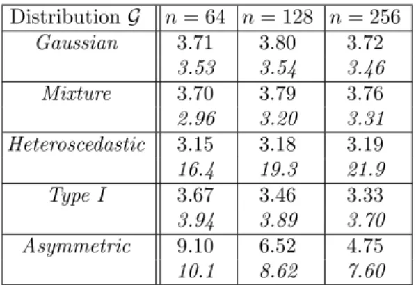
6.2. The level. We first considered the case where F ≡ 0 in order to estimate the level of the tests. For simplicity, the mean of 100 percentages of rejection (as described in Section 6.1) is called here the estimated level. The estimated levels obtained for differentG and n are given in Table 1. Under Gaussian, Mixture and Heteroscedastic the estimated level of our test is, as expected, no greater than the nominal level. Under Type I, the estimated level remains less than the nominal level which means that the method is robust against a slight departure from symmetry. Under Asymmetric, the estimated level is greater than α when n is small and, despite asymmetry, it is smaller than α for n = 256. Even if we cannot explain rigorously this phenomenon, it seems interesting to us to explain it heuristically. Recall that the test consists in selecting a good partition m∗ and
then comparing the distributions of kΠm∗yk2n and kΠm∗(w× y)k2n. If n is large,
then either each subset in m∗ contains a large number of points or the number of
subsets in m∗ is large (or even, the two properties hold simultaneously). If each
subset in m∗ contains a large number of points, then by the central limit theorem
the projections of y and w× y on these subsets have distributions, which are close to Gaussian; if the number of sets in m∗ is large, then the squared norm of the
projections of y and w× y on m∗ (which are sums of projections on the subsets
in m∗) have distributions close to Gaussian. It thus seems that the combination of
two central limit theorems forceskΠm∗yknandkΠm∗(w×y)k to have distributions,
of the εi’s are not symmetric. This explains why the level of our test is less than α
under Asymmetric for large n.
We now compare the performance of our test with that of TP2,Mdya. Under
Gaussian, Mixture, and Type I, the two tests have similar estimated levels and are conservative. Under Heteroscedastic, our test is still conservative while the estimated level of TP2,Mdya is much larger than α, even for large n. Finally, under
Asymmetric, both tests have estimated level larger than α when n is small. But our test performs better than TP2,Mdya, all the more so that n increases. In particular,
our test has the prescribed level when n = 256, whereas TP2,Mdya has not.
Table 1. Estimated level of our test (Roman) and TP1,Mdya (italic) for the five different
distributionsG when α = 5% and n ∈ {64, 128, 256} DistributionG n = 64 n = 128 n = 256 Gaussian 3.71 3.80 3.72 3.53 3.54 3.46 Mixture 3.70 3.79 3.76 2.96 3.20 3.31 Heteroscedastic 3.15 3.18 3.19 16.4 19.3 21.9 Type I 3.67 3.46 3.33 3.94 3.89 3.70 Asymmetric 9.10 6.52 4.75 10.1 8.62 7.60
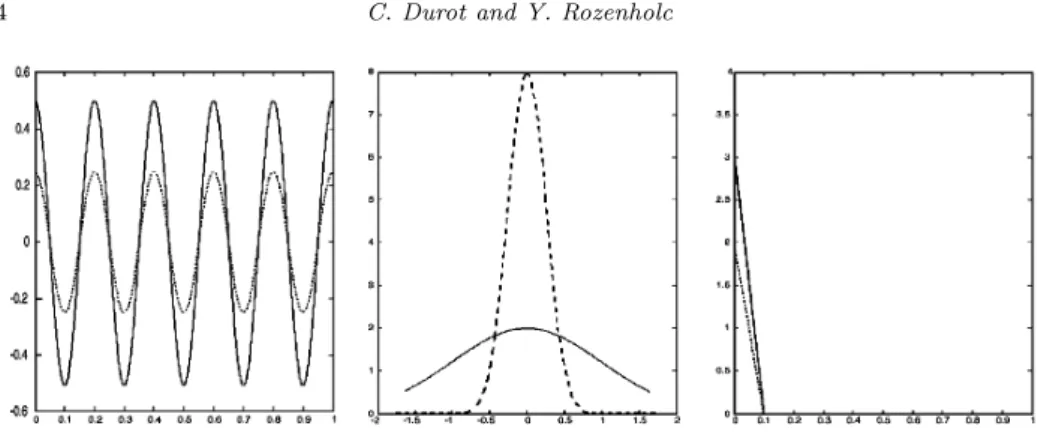
6.3. The power. In this section, we consider cases where F 6≡ 0, so the mean of 100 percentages of rejection (as described in Section 6.1) is called here estimated power. To choose regression functions F , we were inspired by Baraud et al.(2003), where simulations of a test for linearity were performed. To adapt their alternatives to the case of testing for zero regression, we removed the linear part of their functions, so we considered the following functions:
F1k(x) = c1k cos(10πx), k = 1, 2, 3, 4,
F2k(x) = 5 φ(x/c2k)/c2k, k = 1, 2,
F3k(x) =−c3k(x− 0.1)1x≤0.1, k = 1, 2, 3,
where φ is the standard Gaussian density and c11, c12, . . . , c33are equal to 0.25, 0.5,
0.75, 1, 0.25, 1, 20, 30, 40 respectively (see Figure 1). Thus for j∈ {1, 3}, the larger k the farther Fjk is from the null function. In the case of alternatives F1k and F3k
we set xi = (i− 0.5)/n, while for F2k the xi’s are simulated once for all as i.i.d.
centered Gaussian variables with variance 25 in the range [Φ−1(0.05), Φ−1(0.95)],
where Φ is the standard Gaussian distribution function.
Under Gaussian (see Table 2), the two tests have similar power against alter-natives F1k and F2k: the estimated powers are good against F2k and quite small
Figure 1. Alternatives F11, F12 (left), F21, F22 (center) and F31, F32 (right). Alternatives Fj1 and Fj2 are drawn in dotted and plain lines
respectively
against F1k, especially for small values of k and n. The estimated power of TP2,Mdya
is greater than that of our test against F3k, all the more so n is small and k is large
(that is, the signal/noise ratio is large). This is certainly due to the small number of indices i such that F3k(xi) 6= 0. Indeed, our test can detect an alternative if
kΠm∗yk2nis significantly larger thankΠm∗(w× y)k2n for a well chosen partition m∗,
butkΠm∗yk2nremains close tokΠm∗(w× y)k2n if there are only a few indices i such
that yi is significantly different from zero.
Table 2. Estimated power of our test (Roman) and TP
2,Mdya
(italic) under Gaussian distribution. The nominal level is α = 5%
DistributionG Gaussian F F11 F12 F13 F14 F21 F22 F31 F32 F33 n = 64 4.41 8.00 19.4 41.7 99.9 100 12.2 20.2 27.5 4.29 7.78 18.5 39.5 99.8 100 16.2 40.4 72.4 n = 128 6.46 25.0 69.4 96.7 100 100 34.4 70.3 91.2 6.12 24.2 68.2 96.3 100 100 43.3 89.4 99.8 n = 256 12.3 70.1 99.5 100 100 100 84.8 99.9 100 11.7 68.9 99.5 100 100 100 87.8 100 100
Under Mixture or Type I (see Table 3), the estimated powers of the two tests are smaller than under Gaussian, which is due to a greater variance of the errors: under Mixture(resp. Type I), the common variance of the εi’s equals 4.678 (resp. 4). One
can notice however that the signal/noise ratio is the same under Gaussian with F11
(resp. F12, resp. F31) as under Type I with F12 (resp. F14, resp. F33), and is close
to that under Mixture with F12 (resp. F14, resp. F33). Comparing the estimated
powers in these cases shows that, the signal/noise ratio being fixed, both tests have similar powers under these three distributions.
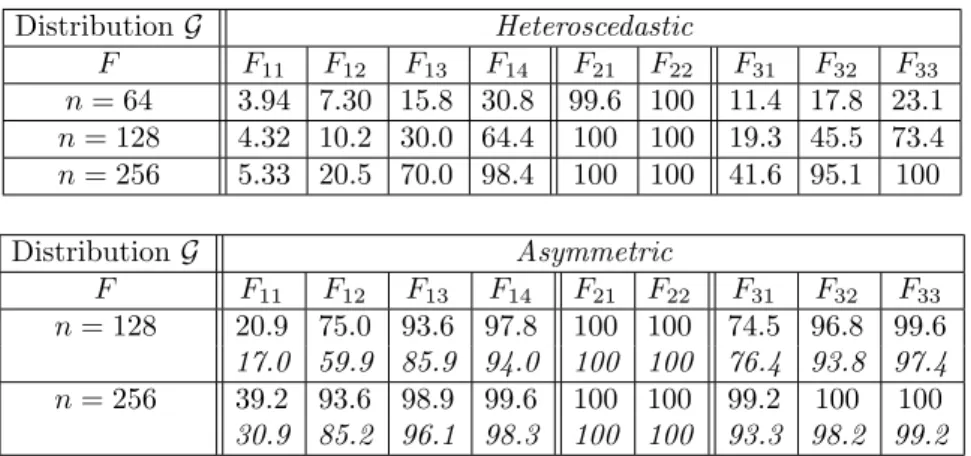
Finally, we studied the power of the two tests under Heteroscedastic and Asym-metric. We give in Table 4 the estimated powers only in the cases where the
Table 3. Estimated power of our test (Roman) and TP
2,Mdya (italic)
under Mixture and Type I distributions. The nominal level is α = 5%
DistributionG Mixture F F11 F12 F13 F14 F21 F22 F31 F32 F33 n = 64 3.93 4.61 6.24 9.32 88.0 98.0 6.15 9.11 12.9 3.12 3.63 4.63 6.80 87.1 97.5 5.06 8.43 14.4 n = 128 4.31 6.63 13.0 25.6 99.8 100 9.74 19.5 34.2 3.60 5.32 10.1 20.5 99.8 100 8.46 18.7 37.3 n = 256 5.16 11.9 31.7 63.4 100 100 18.9 47.1 78.6 4.41 10.0 27.6 59.0 100 100 17.0 45.7 79.5 DistributionG Type I F F11 F12 F13 F14 F21 F22 F31 F32 F33 n = 64 3.88 4.50 5.86 8.68 92.8 99.9 4.99 7.27 10.6 4.15 4.69 5.93 8.38 92.4 99.9 5.67 9.08 15.6 n = 128 3.99 6.21 12.4 26.4 100 100 8.04 17.5 33.8 4.41 6.52 12.3 25.2 100 100 9.25 21.0 43.0 n = 256 4.58 11.8 35.1 70.8 100 100 18.3 51.4 87.3 4.98 11.9 33.9 69.1 100 100 19.3 53.3 88.7
Table 4. Estimated power of our test (Roman) and TP2,Mdya (italic) under Heteroscedastic and
Asymmetricdistributions. The nominal level is α = 5% DistributionG Heteroscedastic F F11 F12 F13 F14 F21 F22 F31 F32 F33 n = 64 3.94 7.30 15.8 30.8 99.6 100 11.4 17.8 23.1 n = 128 4.32 10.2 30.0 64.4 100 100 19.3 45.5 73.4 n = 256 5.33 20.5 70.0 98.4 100 100 41.6 95.1 100 DistributionG Asymmetric F F11 F12 F13 F14 F21 F22 F31 F32 F33 n = 128 20.9 75.0 93.6 97.8 100 100 74.5 96.8 99.6 17.0 59.9 85.9 94.0 100 100 76.4 93.8 97.4 n = 256 39.2 93.6 98.9 99.6 100 100 99.2 100 100 30.9 85.2 96.1 98.3 100 100 93.3 98.2 99.2
estimated level of the test is not much larger than the nominal level. In particular, under Heteroscedastic we only give the estimated power of our test. We can see that the estimated power of our test is smaller under Heteroscedastic than under Gaussian, but remains reasonable. Under Asymmetric, the estimated power of our test is in most cases greater than that of TP2,Mdya, although the estimated level of
In conclusion, our test is powerful against various alternatives (provided the number of indices i such that yi is significantly different from zero is large enough)
and robust against departures from Gaussian distribution and homoscedasticity. It is also robust against slight departures from symmetry.
7. Proofs
Some of the proofs require lemmas. Lemmas are stated when needed and proved in Section 7.8.
7.1. Proof of Theorem 1. Under H0, we have y = ε, so our aim here is to prove that
(16) P¡ sup
m∈M{kΠ
mεk2n− qεm(αm)} > 0¢≤ α.
For every u∈ Rn, let
|u| and sign(u) be the vectors of Rn with ith component
|ui|
and
(17) (sign(u))i = 1{ui≥0}− 1{ui<0},
respectively. The distribution of εi is symmetric about zero and P (εi = 0) = 0,
hence sign(ε) has the same distribution as w and is independent of|ε|. Moreover, w× sign(ε) has the same distribution as w. Since
w× ε = w × sign(ε) × |ε|,
it follows that the distribution of w× ε conditionally on ε is identical to its distri-bution conditionally on|ε|. In particular, qε
m(αm) = qm|ε|(αm), where
q|ε|m(αm) = inf©x∈ R, P [ kΠm(w× ε)k2n > x| |ε| ] ≤ αmª.
But conditionally on |ε|, w × ε has the same distribution as sign(ε) × |ε| = ε. Therefore for every m∈ M,
P¡kΠmεk2n> qmε(αm)| |ε|
¢
= P¡kΠm(w× ε)k2n> qm|ε|(αm)| |ε|
¢ ≤ αm.
Integrating the latter inequality yields
P¡kΠmεk2n > qmε(αm)¢≤ αm.
By assumptionPm∈Mαm= α, hence we get (16). ¤
7.2. Proof of Theorem 2. The first kind error probability of the test with critical region (2) satisfies
P¡ sup m∈M{kΠ mεk2n− bqBm(αm)} > 0¢≤ P£∃m, qεm(αm) <kΠmεk2n ¤ + PBn, where PBn = P£∃m, kΠmεk2n > bqmB(αm) and qεm(αm)≥ kΠmεk2n ¤ .
It thus follows from Theorem 1 that (18) P¡ sup m∈M{kΠmεk 2 n− bqBm(αm)} > 0¢≤ α + PBn. We can have qε
m(αm)≥ kΠmεk2n if and only if pεm> αm, where
pεm= P
¡
kΠm(ω× ε)k2n≥ kΠmεk2n| ε
¢ . Likewise, we can have bqB
m(αm) <kΠmεk2n if and only if 1 B B X b=1 1kΠm(wb×ε)k2n≥kΠmεk2n ≤ αm.
Conditioning with respect to ε thus yields PBn ≤ X m∈M E · P µ 1 B B X b=1 1kΠm(wb×ε)k2 n≥kΠmεk2n≤ αm| ε ¶ 1pε m>αm ¸ . For every m∈ M, let Sε
m be a random variable, which is distributed conditionally
on ε as a binomial variable with parameter B and probability of success pε m. The
Hoeffding inequality yields PBn ≤ X m∈M E£P (Smε ≤ Bαm| ε)1pε m>αm ¤ (19) ≤ X m∈M E£exp(−2B(pεm− αm)2)1pε m>αm ¤ . By dominated convergence, lim B→∞E £ exp(−2B(pε m− αm)2)1pε m>αm ¤ = 0,
so the first part of the theorem follows from (18). In order to prove the second part, we compute the distribution of pε
min the case where the distributions of the
εi’s are continuous (see Section 7.8 for a proof).
Lemma 1. Under the assumptions of Theorem 1 with the additional assump-tion that the distribuassump-tions of the εi’s are continuous, pεm has a discrete uniform
distribution on the set
E =©k2Dm−n, k = 1, . . . , 2n−Dmª.
Combining (19) and Lemma 1 we get PBn ≤ X m∈M µ 2Dm−n X x∈E, x>αm exp(−2B(x − αm)2) ¶ ≤ X m∈M µ 2Dm−n+ Z 1 αm exp(−2B(x − αm)2) dx ¶ . The result now follows from (18) and straightforward computations. ¤
7.3. Proof of Theorem 3. The second kind error probability of the test with critical region (2) satisfies
Pf ¡ sup m∈M{kΠm yk2n− bqBm(αm)} ≤ 0 ¢ ≤ Pf £ ∀m, qmy(δm)≥ kΠmyk2n ¤ + QBn, where QBn = Pf £ ∃m, kΠmyk2n≤ bqBm(αm) and qmy(δm) <kΠmyk2n ¤ .
Using the same arguments as in the proof of Theorem 2 (and also the same notation) we get QBn ≤ X m∈M Ef£Pf(Smy > Bαm| y)1py m≤δm ¤ , where Sy
mis a random variable distributed conditionally on y as a binomial variable
with parameter B and probability of success py
m. By assumption, δm < αm for
all m, so by dominated convergence, QB
n tends to zero as B→ ∞, which proves the
result. ¤
7.4. Proof of Theorems 4 and 5. In this section, we first describe the common line of the proof for the two theorems and then describe the specific arguments for each of them. The lemmas stated in this section are proved in Section 7.8. The following three inequalities are repeatedly used throughout the proof: for all positive real numbers a and b
(20) √a + b≤√a +√b;
for all positive real numbers a, b and θ,
(21) 2√ab≤ θa + θ−1b;
for all positive numbers a, b and k we have (22) (a + b)k ≤ 2k(ak
∨ bk).
Line of proof. Fix β∈ (0, 1) and f ∈ Fn(β). The second kind error probability
of the test at f satisfies Pf¡ sup m∈M{kΠm yk2 n− qym(αm)} ≤ 0¢≤ inf m∈MPf ¡ kΠmyk2n≤ qym(αm)¢.
Therefore, the power of the test is at least 1− β whenever there exists m ∈ M such that
(23) Pf¡kΠmykn2 ≤ qmy(αm)¢≤ β.
Since f ∈ Fn(β), there exists a partition m∈ M such that
(24) kfk2
where ∆ denotes either ∆1 or ∆2. In the sequel, m denotes such a partition. We
aim to prove that (23) holds for this partition, provided the Ak’s are large enough.
Now we show that the subsets em,j which contain only one point cannot contribute
to the power of the test. Let ey∈ Rn with ith component ey
i = 0 if i∈ em,j for an
index j ∈ Jm,1 and eyi = yi otherwise. For every j ∈ Jm,1, let i(j) be the unique
element of em,j. By definition of Πm, kΠmyk2n= X j∈Jm,2 1 |em,j| µ X i∈em,j yi ¶2 + X j∈Jm,1 yi(j)2 =kΠmyek2n+ X j∈Jm,1 yi(j)2 . Let e qym(αm) = inf©x∈ R, Pf¡kΠm(w× ey)k2n> x| y ¢ ≤ αmª. We have wi=±1, so kΠm(w× y)k2n=kΠm(w× ey)k2n+ X j∈Jm,1 y2 i(j), and we get qym(αm) = eqmy(αm) + X j∈Jm,1 y2i(j). Hence (23) amounts to (25) Pf¡kΠmyekn2 ≤ eqmy(αm)¢≤ β,
which means that the sets with only one point can be removed from the condition. Thus we aim to prove that (25) holds provided the Ak’s are large enough. We set
Zm=kΠm(w× ey)k2n= X j∈Jm,2 1 |em,j| µ X i∈em,j wiyi ¶2 and Mm= max j∈Jm,2 ½ 1 |em,j| X i∈em,j y2i ¾ .
We first give an upper bound for eqmy (αm) in order to control the probability in (25).
Lemma 2. e
qmy(αm)≤ Ef(Zm| y) + 8Mmlog(1/αm) + 4
q
2Ef(Zm| y)Mmlog(1/αm).
The obtained upper bound depends on Ef(Zm | y) and Mm, which we have
to control. It is proved in the following two lemmas that with high probability, these variables are not much greater than their expectation. The control we obtain depends on the assumptions on ε.
Lemma 3. Under the assumptions of Theorem1, Pf µ Mm≥ 18(√γ∨ µ ∨ L2) · 1 + 1 Imlog µ3D m β ¶¸¶ ≤β3 and Pf ³ Ef(Zm| y) ≥ Ef(Zm) + 8(√γ∨ L2) p Dmlog(3/β) + 2(µ∨ L2) log(3/β) ´ ≤ β3. Lemma 4. Under the assumptions of Theorem5, there exists an absolute con-stantC≥ 1 such that
Pf µ Mm≥ Cp(µ ∨ L2) · 1 + √1 Im µ 3Dm β ¶1/p¸¶ ≤β3. Moreover, Pf ³ Ef(Zm| y) ≥ Ef(Zm) + 4(µ∨ L2) p 6Dm/β ´ ≤β3.
The main issue to prove Theorems 4 and 5 is to derive from the three lemmas above that (26) Pf ¡ e qmy(αm)≤ Ef(Zm) + Rm ¢ ≥ 1 −2 3β,
where Rmis a positive real number to be chosen later. Then,
(27) Pf ¡ kΠmyek2n≤ eqym(αm) ¢ ≤ 2 3β + Pf ¡ kΠmyek2n≤ Ef(Zm) + Rm ¢ ,
and it remains to prove that the right-hand side probability is less than or equal to β/3. In order to do that, we state a concentration inequality which proves that with high probability, kΠmyek2n is not much smaller than its expectation. Here
again, the obtained control depends on the assumptions on ε. In the sequel, ef denotes the expectation of ey.
Lemma 5. Under the assumptions of Theorem5,
Pf µ kΠmyek2n≤ EfkΠmeyk2n−6 s γDm β − 1 3kΠmfek 2 n−14(√γ∨µ∨L2) log µ 6 β ¶¶ ≤ β3. Lemma 6. Under the assumptions of Theorem5,
Pf µ kΠmeyk2n≤ EfkΠmyek2n− 3µ s Dm β − 1 3kΠmfek 2 n− 9µ β ¶ ≤β3.
In both cases, there is R′ m≥ 0 such that (28) Pf ³ kΠmyek2n ≤ EfkΠmyek2n− R′m− 1 3kΠmfek 2 n ´ ≤β3.
Thus the right-hand side probability in (27) is less than or equal to β/3 as soon as (29) Ef(Zm) + Rm≤ EfkΠmeyk2n− R′m−
1 3kΠmfek
2 n,
hence it suffices to prove (29). By assumption, the wi’s and the yi’s are
mutu-ally independent, and the distribution of wi is symmetric about zero. Therefore,
E(wi) = 0 and the random variables wiyiare mutually independent with zero mean
and variance Ef(y2i) = E(ε2i) + fi2. Hence,
(30) Ef(Zm) = X j∈Jm,2 1 |em,j| X i∈em,j (E(ε2i) + fi2).
We have|em,j| ≥ Im for all j∈ Jm,2, so
EfkΠmeyk2n− Ef(Zm) = X j∈Jm,2 1 |em,j| µ X i∈em,j E(ε2i) + ³ X i∈em,j fi ´2 − X i∈em,j (E(ε2i) + fi2) ¶ ≥ X j∈Jm,2 1 |em,j| µ X i∈em,j fi ¶2 −I1 m X j∈Jm,2 X i∈em,j fi2. Hence EfkΠmyek2n− Ef(Zm)≥ kΠmfk2n− |Jm,1| max 1≤i≤nf 2 i − 1 Imkfk 2 n.
In order to prove (29), it suffices to prove
(31) 2 3kΠmfk 2 n≥ 1 Imkfk 2 n+|Jm,1| max 1≤i≤nf 2 i + Rm+ R′m.
By definition, Im≥ 2 and by the Pythagoras equality,
(32) kΠmfk2n=kfk2n− kf − Πmfk2n.
Thus it suffices to prove 1 6kfk 2 n≥ 2 3kf − Πmfk 2 n+|Jm,1| max 1≤i≤nf 2 i + Rm+ R′m.
But f satisfies (24), so it suffices to check that for large enough Ak,
(33) ∆(m, f, A)≥ 4kf − Πmfk2n+ 6 © |Jm,1| max 1≤i≤nf 2 i + Rm+ R′m ª .
Now to prove Theorems 4 and 5, it remains to compute Rm and R′m and to
check (33) with ∆ replaced by ∆1 and ∆2respectively.
Proof of Theorem4. By (30),
Ef(Zm)≤ Dm(
p
2γ + L2).
Using (21) we thus get Ef(Zm) + 8(√γ∨ L2)
p
Dmlog(3/β) + 2(µ∨ L2) log(3/β)
≤ 7(√γ∨ µ ∨ L2)¡D
m+ log(3/β)¢.
Combining Lemmas 2 and 3 proves that with probability greater than 1− 2β/3, e qmy(αm)≤ Ef(Zm) + 8(√γ∨ L2) p Dmlog(3/β) + 2(µ∨ L2) log(3/β) + 144(√γ∨ µ ∨ L2) · 1 + 1 Im log µ3D m β ¶¸ log µ 1 αm ¶ + 24(√γ∨ µ ∨ L2) s 7 µ Dm+ log µ 3 β ¶¶µ 1 + 1 Im log µ 3Dm β ¶¶ log µ 1 αm ¶ . Using (20) and (21), we get that with probability greater than 1− 2β/3,
e qmy(αm)≤ Ef(Zm) + 8(√γ∨ L2) p Dmlog(3/β) + 151(√γ∨ µ ∨ L2) log(3/β) + 151(√γ∨ µ ∨ L2) · 1 + 1 Im log µ 3Dm β ¶¸ log µ 1 αm ¶ + 24(√γ∨ µ ∨ L2) s 7Dm · 1 + 1 Im log µ 3Dm β ¶¸ log µ 1 αm ¶ . By assumption, log(1/αm) and log(3/β) are positive, so we obtain (26) with
Rm= 151(√γ∨ µ ∨ L2) · 1 + 1 Im log µ3D m β ¶¸ log µ 3 βαm ¶ + 72(√γ∨ µ ∨ L2) s Dm · 1 + 1 Im log µ 3Dm β ¶¸ log µ 3 βαm ¶ . By Lemma 5, we have (28) with
R′m= 6
p
γDm/β + 14(√γ∨ µ ∨ L2) log(6/β),
so (33) holds with ∆ replaced by ∆1provided A1, . . . , A5 are large enough. ¤
Proof of Theorem5. By (30),
Combining Lemmas 2 and 4 proves that with probability greater than 1− 2β/3, e qmy(αm)≤ Ef(Zm) + 4(µ∨ L2) s 6Dm β + 8Cp(µ∨ L2) · 1 +√1 Im µ 3Dm β ¶1/p¸ log µ 1 αm ¶ + 18(µ∨ L2) v u u tCpµDm+ s Dm β ¶· 1 +√1 Im µ3D m β ¶1/p¸ log µ 1 αm ¶ . Using (20) and (21), we get (26) with
Rm= 19(µ∨ L2) s Dm β + 17Cp(µ∨ L 2) · 1 + √1 Im µ 3Dm β ¶1/p¸ log µ 1 αm ¶ + 18(µ∨ L2) s CpDm · 1 + √1 Im µ 3Dm β ¶1/p¸ log µ 1 αm ¶ . By Lemma 6, we have (28) with
R′m= 3µ
p
Dm/β + 9µ/β,
so (33) holds with ∆ replaced by ∆2provided A1, . . . , A6 are large enough. ¤
7.5. Proof of Corollary 1. We define δ and δ′ in the following way. If (4) holds for all p≥ 1 and some γ and µ, we set δ = δ′ = √γ + µ + L2. If (5)
holds for some p≥ 2 and some µ, we set δ =√p(µ + L2) and δ′ = p(µ + L2). By
Step 2 in the proof of Corollary 1 of Baraud et al. (2003), kf − Πmkfk
2
n≤ nR2k−2s
for all k ∈ I. Moreover, |M| ≤ log n/ log 2, so there exists cα > 0, which only
depends on α, such that
log(1/αm)≤ cαlog log n.
We have (12) and Dmk ≤ k for all k ∈ I, so it follows from Theorem 4 that the
power of the test is greater than 1− β whenever (4) holds and kfk2 n≥ A inf k∈I ½ nR2k−2s+ δ µ 1 + k nlog n ¶ log log n (34) + δ s k µ 1 + k nlog n ¶ log log n ¾ ,
for a large enough A. Likewise, it follows from Theorem 5 that the power of the test is greater than 1− β whenever (5) holds and
kfk2n ≥ A inf k∈I ½ nR2k−2s+ δ′ µ 1 +k 1/p+1/2 √n ¶ log log n (35) + δ s k µ 1 + k 1/p+1/2 √n ¶ log log n ¾
for a large enough A. In (34) and (35), A > 0 only depends on a, a0, α, and β. In
the sequel,I′ denotes the subset of
I defined as follows. Under (4), I′ is the set of
those k ∈ I, which satisfy k log n ≤ n and under (5), I′ is the set of those k
∈ I, which satisfy k1/p+1/2≤√n, that is k≤ np/(p+2).
• Assume first that (4) and 1 (a), resp. (5) and 2 (a), hold for a large enough C. By (34) and (35), the power of the test is greater than 1− β whenever
kfk2 n≥ 2A h inf k∈I′ ©
nR2k−2s+ δpk log log nª+ δ′log log ni. Let (36) k∗= µ nR2 δ√log log n ¶2/(1+4s) . We have nR2k−2s≤ δpk log log n
if and only if k ≥ k∗ and for large enough n, there exists k′ ∈ I′ such that k∗ ≤
k′ ≤ 2k∗. Therefore,
inf
k∈I′
©
nR2k−2s+ δpk log log nª≤ 2δpk′log log n
≤ 4δpk∗log log n≤ 4nR2/(1+4s) µ δ√log log n n ¶4s/(1+4s) .
The power of the test is thus greater than 1− β whenever n is large enough and kfk2 n≥ 2A · 4nR2/(1+4s) µ δ√log log n n ¶4s/(1+4s) + δ′log log n ¸ .
This indeed holds if n is large enough and either 1 (a) or 2 (a) is fulfilled for a large enough C.
• Assume (4). By (34), the power is greater than 1 − β whenever n is large enough and (37) kfk2 n≥ 3A inf k∈I\I′ ½ nR2k−2s+ δk r 1
nlog n× log log n ¾
for a large enough A. Let k∗=
µ n3/2R2
δ√log n× log log n
¶1/(1+2s)
.
If s = 1/4 and n is large enough, there exists k′∈ I \ I′ such that k
∗≤ k′≤ 2k∗. Therefore, inf k∈I\I′ ½ nR2k−2s+ δk r 1
nlog n× log log n ¾
≤ 4δk∗
r 1
The power of the test is thus greater than 1− β whenever n is large enough and 1 (b) holds for a large enough C. Let k0 be a point inI with k0≥ n/8. Then (37)
holds whenever kfk2 n≥ 3A ½ nR2k−2s 0 + δk0 r 1
nlog n× log log n ¾
.
Since k0≤ n/2, this indeed holds if n is large enough and 1 (c) is fulfilled for a large
enough C.
• Assume (5) holds for some p ≥ 2. If n is large enough, we have for all k ≥ 1 δ′k1/p+1/2n−1/2log log n
≤ δk1/2p+3/4n−1/4plog log n.
By (35), the power is thus greater than 1− β whenever n is large enough and (38) kfk2n≥ 4A inf k∈I\I′ n nR2k−2s+ δk1/2p+3/4n−1/4plog log no. Let k∗= µ n5/4R2 δ√log log n ¶4p/(2+3p+8ps) . If s∈ [1/4 − 1/p, 1/4 + 1/p) and n is large enough, there exists k′
∈ I \ I′such that k∗≤ k′≤ 2k∗. Therefore, inf k∈I\I′ n nR2k−2s+ δk1/2p+3/4n−1/4plog log no≤ 4δk1/2p+3/4∗ n−1/4 p log log n. The power of the test is thus greater than 1− β whenever n is large enough and 2 (b) holds for a large enough C. Let k0 be a point inI with k0≥ n/8. Then (38)
holds whenever kfk2 n ≥ 4A n nR2k−2s 0 + δk 1/2p+3/4 0 n−1/4 p log log no.
This indeed holds if n is large enough and 2 (c) is fulfilled for a large enough C. ¤ 7.6. Proof of Corollary 2. Let k∗ be given by (36) and let k′ ∈ I be such that k∗ ≤ k′ ≤ 2k∗ (such a k′ exists provided n is large enough). By
Theorems 4 and 5, it suffices to prove that kfk2
n exceeds ∆(mk′, f, A) for large
enough n and a fixed A, where ∆ denotes either ∆1or ∆2. By (31), one can choose
A1=
2/3 2/3− 1/Imk′
.
Moreover, there exists A0> 0, which only depends on α, β, and A such that
∆(mk′, f, A)≤ A1kf − Πmfk2n+ A0δ
p
By (32), it thus suffices to show that for large enough n, (39) kΠmk′fk 2 n≥ 3 2Imk′ kfk2n+ A0δ p k′log log n.
We need further notation. Let Fn be the function defined by Fn(t) = F (xi) for all
t ∈ (xi−1, xi], i = 1, . . . , n, where we set xi = i/n for all i = 0, . . . , n. For every
j = 0, . . . , k′, let tj= 1 n X i≤j |emk′,i| = 1 n ·nj k′ ¸
(here, [x] denotes the integer part of x). Let Q be the orthogonal projector from L2[0, 1] onto the set of step functions, which are constant on each interval (tj−1, tj],
and let Qrbe the orthogonal projector from L2[0, 1] onto the set of step functions,
which are constant on each interval ((j−1)/k′, j/k′], j = 1, . . . , k′. Since t
j−1−tj≤ 2/k′ and |tj− j/k′| ≤ 1/n, we have kQF k2 2= k′ X j=1 1 tj− tj−1 µ Z tj tj−1 F (x) dx ¶2 ≥ 14kQrFk22− 2k′2 kF k2 ∞ n2
(recall that (a + b)2≥ a2/2− b2 for all real numbers a and b). Now,
kQ(F − Fn)k2≤ kF − Fnk2≤ kF − Fnk∞≤ kF′k∞/n and we have kΠmk′fkn=√nkQFnk2. Therefore, kΠmk′fkn ≥ √ nkQF k2− kF′k∞/√n≥ √n 2 kQrFk2− √ 2k′ kF k∞ √n − kF′ k∞/√n.
The partition of [0, 1] associated with Qris equispaced (all intervals have the same
length 1/k′), so one can prove that there exist positive numbers C
1 and C2, which
only depend on s, such that
kQrFk2≥ C1kF k2− C2Rk′−s,
see Proposition 2.16 of Ingster and Suslina (2003). It then follows from the definition of k′and the assumption s > 1 that there exist positive numbers C′
1 and C2′, which
only depend on s, such that for large enough n, kΠmk′fkn≥ C
′
1√nkF k2− C2′√nRk′−s.
Note that
and that Imk′ tends to infinity as n goes to infinity. Thus in order to prove (39), it
suffices to prove that for large enough n and some A′ 0> 0, kF k22≥ A′0 ½ R2k′−2s+ δ n p k′log log n ¾ .
But this is indeed the case if F satisfies (15) for a large enough C > 0. ¤ 7.7. Power in a Gaussian homoscedastic model. In this section, we assume that the εi’s are i.i.d.N (0, σ2) and|fi| ≤ σL for all i. We will prove that
the power of the test is greater than 1− β whenever f satisfies (7) for large enough Ak’s. Under the above assumptions, Lemmas 2 and 3 are valid with µ = 2σ2,
γ = µ2, and L2replaced by σ2L2. In particular, we have (26) with
Rm= 302σ2(1 + L2) · 1 + 1 Imlog µ3D m β ¶¸ log µ 6 βαm ¶ + 144σ2(1 + L2) s Dm · 1 + 1 Im log µ 3Dm β ¶¸ log µ 6 βαm ¶ .
Moreover, one can improve the result given in Lemma 5 under the Gaussian as-sumption, due to the Cochran theorem. Indeed, let D′
m denote the cardinality
of Jm,2. By the Cochran Theorem, kΠmeyk2n/σ2 is a non-central χ2 variable with
D′
mdegrees of freedom and non-centrality parameterkΠmfek2n/σ2. By Lemma 1 of
Birg´e (2001), we thus have for all positive x
Pf · 1 σ2kΠmyek 2 n ≤ 1 σ2EfkΠmyek 2 n− 2 sµ D′ m+ 2 σ2kΠmfek2n ¶ x ¸ ≤ exp(−x). Using (20) and (21) one obtains
Pf h kΠmyek2n ≤ EfkΠmyek2n− 2σ2 p D′ mx− 1 3kΠmfek 2 n− 6σ2x i ≤ exp(−x), for all x > 0. Setting x = log(3/β) in this inequality yields
Pf · kΠmyek2n≤ EfkΠmyek2n− 2σ2 s Dmlog µ 3 β ¶ −13kΠmfek2n− 6σ2log µ 3 β ¶¸ ≤ β3. Therefore, we have (28) with
R′m= 2σ2
p
Dmlog(3/β) + 6σ2log(3/β).
Let ∆(m, f, A) denote the bracketed term in (7). Then (32) holds provided the Ak’s are large enough, which proves the announced result. ¤
7.8. Proof of the lemmas. We first recall two inequalities, which will be used in this section.
Bernstein’s Inequality. Let X1, . . . , Xn be independent real-valued random
variables. Assume that there exist positive numbersv and c such that for all integers k≥ 2 n X i=1 E[|Xi|k]≤ k! v 2c k−2.
Let S =Pni=1(Xi− E[Xi]). Then for every x > 0, P
£
S ≥√2vx + cx¤≤ exp(−x). Rosenthal’s Inequality. Let X1, . . . , Xn be independent centered real-valued
random variables with finitet-th moment, 2≤ t < ∞. Then there exists an absolute constant L such that
E¯¯¯ n X i=1 Xi ¯ ¯ ¯ t ≤ Ltttmax µXn i=1 E|Xi|t, ³Xn i=1 E|Xi|2 ´t/2¶ .
Proof of Lemma1. For notational convenience, we omit subscript m. For every j = 1, . . . , D and z∈ Rn, define the set
Aj(z) byAj(z) ={0} if D = 1 and Aj(z) = ½ X k6=j 1 |ek| ³ X i∈ek uizi ´2 , u∈ {±1}n ¾
if D > 1. For every j = 1, . . . , D let
Ej ={e ⊂ ej s.t. e6= ∅ and e 6= ej}. Finally, let Y = D \ j=1 n
z∈ Rn s.t. ∀u ∈ {±1}n,∀a, a′∈ Aj(z),∀e ∈ Ej,
4X i∈e uizi X i∈ej\e uizi6= (a′− a)|ej| o .
The εi’s are independent and all have a continuous distribution, so the event
{ε ∈ Y} is the intersection of a finite number of events having probability one. We thus assume in the sequel without loss of generality that ε ∈ Y. Let u and u′ be
elements of{±1}n such that
(40) kΠ(u × ε)k2n=kΠ(u′× ε)k2n. Fix j∈ {1, . . . , D}. We have 0 =kΠ(u × ε)k2 n− kΠ(u′× ε)k2n= 1 |ej| ·³ X i∈ej uiεi ´2 −³ X i∈ej u′iεi ´2¸ + a− a′ for some a, a′ ∈ Aj(ε). Setting e ={i ∈ ej s.t. ui= u′i} we get ³ X i∈ej uiεi ´2 −³ X i∈ej u′iεi ´2 =X i∈ej (ui+ u′i)εi X i∈ej (ui− u′i)εi= 4 X i∈e uiεi X i∈ej\e uiεi,
since ui=−u′i for every i∈ ej\ e. As ε ∈ Y, either e = ∅ or e = ej. Thus for all
j = 1, . . . , D, either ui = u′i for all i∈ ej or ui =−u′i for all i∈ ej. This implies
that the cardinality of the set ©
kΠ(u × ε)k2
n, u∈ {±1}n
ª
is 2n−D and that for every element a of this set, the cardinality of the set
©
u∈ {±1}n s.t. a =kΠ(u × ε)k2n
ª is equal to 2D. This proves that conditionally on ε,
kΠ(w × ε)k2
n has a discrete
uniform distribution on a set with 2n−D distinct values. Clearly,
kΠεk2
n belongs
to this set, so pε = k2D−n for some k = 1, . . . , 2n−D. More precisely, we have
pε= k2D−nif and only if the cardinality of the following set is equal to k:
©
kΠ(u × ε)k2
n s.t. kΠ(u × ε)k2n ≥ kΠεk2n, u∈ {±1}n
ª . But this set has the same cardinality as the set
©
kΠ(u × |ε|)k2
n s.t. kΠ(u × |ε|)k2n ≥ kΠ(sign(ε) × |ε|)k2n, u∈ {±1}n
ª , where we recall that sign(ε) is the vector in Rn defined by (17). Since sign(ε) has
the same distribution as w and is independent of |ε| (see the proof of Theorem 1) we get P (pε= k2D−n | |ε|) = P³ X u∈{±1}n 1kΠ(u×|ε|)k2 n≥kΠ(w×|ε|)k2n = k| |ε| ´ . Moreover conditionally on|ε|, kΠ(w × |ε|)k2
nhas a uniform discrete distribution on
a set with 2n−D distinct values. Therefore,
P¡pε= k2D−n| |ε|¢= 2D−n. Integrating this inequality yields the result. ¤
Proof of Lemma 2. First, note that Lemma 2 is trivial whenever eyi = 0 for all
i since in that case eqy
m(αm) = 0. We thus assume in the sequel that there exists i
such that eyi6= 0. In particular, Mm> 0. Now, note that Zmcan be written as the
sum of squared random variables: Zm=
X
j∈Jm,2
X2 j,
where for every j∈ Jm,2,
Xj = X i∈J wiyi p |em,j| 1em,j(i).
Here,
(41) J = [
j∈Jm,2
em,j.
Denote by Sm the unit sphere in R|Jm,2|. Then
Zm1/2= sup a∈Sm X j∈Jm,2 ajXj = sup a∈Sm X i∈J wi yiaj(i) p |em,j(i)| ,
where for every i, j(i) denotes the unique integer in Jm,2 that satisfies i∈ em,j(i).
If S′
mdenotes a finite subset of Sm, then it follows from a result of Massart (2006)
that for all x≥ 0, Pf · sup a∈S′ m X j∈Jm,2 ajXj≥ Ef ³ sup a∈S′ m X j∈Jm,2 ajXj | y ´ + x| y ¸ ≤ exp µ − x 2 8σ2(S′ m) ¶ , where σ2(S′m) = sup a∈S′ m X i∈J y2 ia2j(i) |em,j(i)| = sup a∈S′ m X j∈Jm,2 a2 j |em,j| X i∈em,j y2i.
But Sm is separable and for every subset Sm′ of Sm, σ2(Sm′ )≤ Mm. Hence for all
x≥ 0, Pf £ Zm1/2≥ Ef(Zm1/2| y) + x | y ¤ ≤ exp(−x2/8Mm). In particular, Pf£Zm1/2≥ Ef(Zm1/2| y) + p 8Mmlog(1/αm)| y¤≤ αm.
Squaring the inequality yields Pf h Zm≥ Ef2(Zm1/2| y) + 8Mmlog(1/αm) + 2Ef(Zm1/2| y) p 8Mmlog(1/αm)| y i ≤ αm. By definition of eqy m(αm) we thus have e qym(αm)≤ Ef2(Zm1/2| y) + 8Mmlog(1/αm) + 2Ef(Zm1/2| y) p 8Mmlog(1/αm),
and the result follows from the Jensen inequality, which implies Ef2(Zm1/2| y) ≤ Ef(Zm| y). ¤
Proof of Lemma3. By definition of Mm, we have for all real numbers x and c
Pf£Mm≥ c + x ¸ ≤ X j∈Jm,2 Pf · 1 |em,j| X i∈em,j yi2≥ c + x ¸ .
In particular, if c is large enough so that Ef(y2i)≤ c for all i, then for all x (42) Pf £ Mm≥ c + x ¤ ≤ X j∈Jm,2 Pf · 1 |em,j| X i∈em,j ¡ y2i − Ef(yi2) ¢ ≥ x ¸ . Let p≥ 1. By (22), y2pi ≤ 22p(ε 2p i ∨ L2p) and in particular, y 2p i ≤ 22p(ε 2p i + L2p). Therefore, (43) Ef(yi2p)≤ 2 2p+1max©γp!µp−2, L2pª ≤ γ0p!µp−20 ,
where γ0= 25(γ∨ L4) and µ0= 4(µ∨ L2). By Bernstein’s inequality, we thus have
for all x≥ 0 Pf · X i∈em,j ¡ y2i − Ef(y2i) ¢ ≥ 2qγ0|em,j|x + µ0x ¸ ≤ exp(−x). Moreover, Ef(y2i)≤ L2+ √2γ, so by (42), Pf · Mm≥ p 2γ + L2+ 2 rγ 0x Im +µ0x Im ¸ ≤ Dmexp(−x). We have p 2γ + L2+ 2 rγ 0x Im + µ0x Im ≤ p 2γ + L2+ (2√γ0+ µ0) µ 1 + x Im ¶ ≤ 18(√γ∨ µ ∨ L2) µ 1 + x Im ¶ . Hence for all x > 0,
Pf · Mm≥ 18(√γ∨ µ ∨ L2) µ 1 + x Im ¶¸ ≤ Dmexp(−x).
Setting here x = log(3Dm/β) yields the first assertion in Lemma 3. The variables wi
are independent with mean zero and variance 1, and these variables are independent from y. Hence conditionally on y, they are still independent with mean zero and variance 1, and we derive from the definition of Zmthat
(44) Ef(Zm| y) = X j∈Jm,2 1 |em,j| X i∈em,j y2i. By (43), X j∈Jm,2 X i∈em,j Ef ·µ y2 i |em,j| ¶p¸ ≤Dm2γ0p! µµ 0 2 ¶p−2 , so Bernstein’s inequality yields for all x≥ 0
Pf h Ef(Zm| y) ≥ Ef(Zm) + p 2Dmγ0x +1 2µ0x i ≤ exp(−x). Setting here x = log(3/β) completes the proof of the lemma. ¤
Proof of Lemma 4. By Rosenthal’s inequality, there exists an absolute constant C′> 0 such that for all j
Ef ¯ ¯ ¯ X i∈em,j (yi2− Ef(y2i)) ¯ ¯ ¯ p ≤ (C′p)pmaxn X i∈em,j Ef|yi2− Ef(y2i)|p, ³ X i∈em,j var(y2 i) ´p/2o .
Moreover, by Jensen’s inequality, Eε4
i ≤ µ2for all i, so by (22), varf(yi2)≤ Ef(yi4)≤ 24(µ2+ L4). Hence, ³ X i∈em,j varf(yi2) ´p/2 ≤ 25p/2 |em,j|p/2(µp∨ L2p).
On the other hand, X i∈em,j Ef|y2i−Ef(yi2)|p≤ 2p X i∈em,j £ Ef(yi2p)+|Ef(y2i)|p ¤ ≤ 2p+1+2p|em,j|(µp+L2p), so we get Ef ¯ ¯ ¯ X i∈em,j (y2 i − Ef(yi2)) ¯ ¯ ¯ p ≤ (Cp)p |em,j|p/2(µp∨ L2p),
where for instance C = 24C′. We have E
f(y2i) ≤ µ + L2, so (42) and Markov’s inequality yield Pf£Mm≥ µ+L2+x¤≤ (Cp)p(µp∨L2p) X j∈Jm,2 1 xp|e m,j|p/2 ≤ (Cp) p(µp ∨L2p) Dm xpIp/2 m
for all x > 0. In particular, Pf · Mm≥ µ + L2+ Cp(µ∨ L2) 1 √ Im µ 3Dm β ¶1/p¸ ≤ β3.
We can assume without loss of generality that C ≥ 1, so the first assertion of Lemma 4 follows. We have (44), where the yi’s are independent. Therefore,
varf£Ef(Zm| y)¤≤ max 1≤i≤nEf(y
4
i)Dm≤ 24(µ2+ L4)Dm.
Now the second assertion of the lemma follows from the Bienaym´e–Chebyshev in-equality. ¤
Proof of Lemma5. LetJ be defined by (41). We have kΠmyek2n =kΠmeεk2n+kΠmfek2n+ 2 X j∈Jm,2 1 |em,j| ³ X i∈em,j εi ´³ X i∈em,j fi ´ ,