HAL Id: hal-00907402
https://hal.archives-ouvertes.fr/hal-00907402
Submitted on 21 Nov 2013
HAL is a multi-disciplinary open access archive for the deposit and dissemination of sci-entific research documents, whether they are pub-lished or not. The documents may come from teaching and research institutions in France or abroad, or from public or private research centers.
L’archive ouverte pluridisciplinaire HAL, est destinée au dépôt et à la diffusion de documents scientifiques de niveau recherche, publiés ou non, émanant des établissements d’enseignement et de recherche français ou étrangers, des laboratoires publics ou privés.
Hemodynamics
Olivier Pironneau
To cite this version:
Olivier Pironneau. Simplified Fluid-Structure Interactions for Hemodynamics. Numerical Simulations of Coupled Problems in Engineering, 33, Springer Verlag, pp.57-70, 2014, Springer series Computa-tional Methods in Applied Sciences. �hal-00907402�
SIMPLIFIED FLUID-STRUCTURE INTERACTIONS FOR
HEMODYNAMICS
Olivier Pironneau⋆
⋆ Laboratoire Jacques-Louis Lions, Universit´e Pierre et Marie Curie (Paris VI), Boite courrier
187, 75252 Paris Cedex 05. France. [email protected]
Key words: Blood flow, hemodynamics finite element method, pressure boundary con-ditions, Primary: 91B28, 65L60; Secondary: 82B31
Abstract. Computing blood flows in a closed vascular system by isolating one section for simulation creates difficulties due to the time-periodic structure of the flow and possible non-physical back flow in the simplified geometry.
We propose some solutions in the context of a simplified fluid structure interaction on a fixed geometry but with pressure dependent normal velocities at the compliant walls. The present analysis is based on the Surface Pressure model for the fluid-structure inter-actions.
1 Introduction
Mastering the simulation of blood flow is the key to proper design of by-passes, stents and heart valves (see Thiriet[18] for instance).
The problem was addressed by Charles Peskin in the nineties and his team have made impressive simulations since using fictitious domains and immersed boundary techniques [14, 13, 19, 1].
Another approach, taken by Quarteroni et al [6] and the REO project at INRIA [5, 4, 20] is to discretize the full fluid-structure coupled problem with solvers working in moving domains.
In a seminal paper [12], Nobile and Vergana showed that the problem is well posed and conserves energy. Nevertheless the numerical simulations are expensive [2] and there is room for simplifications.
In the special case of aortic flow the geometry does not change much. Typically the aorta has a radius of 1cm and a computational geometry deals with a section of length of 5 to 10 centimeters; the thickness of the aortic wall is around 0.1cm; the heart pulse is about 1Hz and the pressure drop roughly 6KPa.
In principle arteries are deformable solids subject to large displacements and nonlinear elasticity (e.g.[8, 9, 11]). But when small displacement occurs only and linear elastic-ity applies, shell models like Koiter’s can be used. It was shown in [12] that if lateral displacements are neglected, Koiter’s model reduces to a scalar equation for the normal displacement η
ρsh∂ttη − ∇ · (T∇η) − ∇ · (C∇∂tη) + a∂tη + bη = fs, η, ∂tη given at t = 0 (1)
on the mean position Σ of the vessel’s wall; here h denotes the average thickness of the vessel and ρs its volumic mass; T is the pre-stress tensor (needed because at rest the
vessel is blown up by the blood ); C is a damping term, a, b are viscoelastic terms and fs
the external normal force, i.e. −σs
nn the normal component of the normal stress at the
surface of the solid.
Notice however that the other components of the normal stress tensor cannot be matched with the fluid when the displacement is assumed normal.
Finally ssume that [h, T, C, a] << b; then the Surface Pressure Model is obtained: −σsnn = bη, with b =
Ehπ
A(1 − ξ2) (2)
where A is the vessel’s cross section, E the Young modulus, ξ the Poisson coefficient. Some typical values (MKSA):
E = 3M P a, ξ = 0.3, A = πR2, R = 0.01, h = 0.001, ⇒ b = 3.3107ms−2
2 Boundary Conditions
With simple toroidal coordinates (r, θ, φ) → (x = R cos φ, y = R sin φ, z = r sin θ) where R = R0 + r cos θ, ∇ · u = hrhθhφ(∂r ur hθhφ + ∂θ uθ hφhr + ∂φ uφ hrhθ ) (4)
with hr = 1, hθ = 1r, hφ= R1 because, by definition
1 h2 k = (∂kx)2+ (∂ky)2+ (∂kz)2, k = r, θ, φ (5) So ∇ · u = 0 and u × n = 0 imply ∇ · u = ∂rur+ ur R0+ 2r cos θ r(R0+ r cos θ) = 0 ⇒ ∂rur|∂Ω = − ur r R0+ 2r cos θ R0+ r cos θ (6) Similarly ∇u =X i eih i⊗ ∂k( X k eku k), i, k ∈ (r, θ, φ) (7) with
er = (cos θ cos φ, cos θ sin φ, sin θ)T,
eθ = (− sin θ cos φ, −sinθ sin φ, cos θ)T, eφ= (− sin φ, cos φ, 0)T (8)
Thus nT(∇u)n = ∂ rur+ ur r (1 + r Rcos 2θ) ⇒ σf nn = p + 2(1 + r R cos 2θ)µ ru · n. (9) Hence the matching conditions at the fluid-structure interface on a torus of small radius r and big radius R are
∂tη = u · n, p = 2(1 +
r Rcos
2θ)µ
r∂tη + bη (10) Notice that (10) implies
∂tp = 2(1 +
r Rcos
2θ)µ
r∂tu · n + bu · n (11) Equation (19) and the above lead to the following problem:
3 Moving Fluid Domains versus Fixed Domains 3.1 Energy Considerations
Assuming the fluid Newtonian and incompressible, the pressure p and the velocity u are given by the Navier-Stokes equations
ρf(∂u
∂t + u · ∇u) − ∇ · σ
f
= 0, ∇ · u = 0, (12) where ρf is the volumic mass of the fluid, µ the viscosity and σf = −pI + µ(∇u + ∇uT)
is the stress tensor.
To check the energy budget one multiplies (12) by u and integrates by parts: Z Ω [ρ f 2 ∂t|u| 2+µ 2(∇u + ∇u T ) : (∇u + ∇uT)] + Z ∂Ω ρf 2 |u| 2u · n = Z ∂Ω σs· u. (13) The fluid velocity on ∂Ω is equal to the wall velocity, so (see [6])
Z Ω(t) 1 2∂t|u| 2 + Z ∂Ω 1 2|u| 2u · n = ∂ t Z Ω(t) 1 2|u| 2 (14)
This leads to the following energy identity Z Ω(T ) ρf 2|u| 2(T ) + Z Ω×(0,T ) µ 2|∇u + ∇u T |2 = Z Ω(0) ρf 2|u| 2(0) + Z ∂Ω×(0,T ) σs· u. (15) 3.2 The problem in Strong form
Now if we consider (12) on a fixed domain with zero tangential velocities but non-zero normal velocities on the walls then to conserve energy we need to change u · ∇u into u · ∇u − 1
2∇|u|
2 which happens to be −u × ∇ × u due to the identity
u · ∇u = 1 2∇|u|
2− u × ∇ × u. (16)
Let us recall another identity:
−∆u = ∇ × ∇ × u + ∇∇ · u (17) Therefore the modified Navier-Stokes system suited to flows in fixed domains with zero tangential components on the walls (u × n = 0) is
ρf(∂u
∂t − u × ∇ × u) + µ∇ × ∇ × u + ∇p = 0, ∇ · u = 0, (18) In a domain Ω with u · n = 0 and p related by (11) on ∂Ω, as shown below.
3.3 The problem in Variational Form
Its variational formulation of is: find u, p such that ∀ˆu, ˆp with ˆu × n|∂Ω = 0,
Z Ω [ρf(∂u ∂t − u × ∇ × u) · ˆu + µ∇ × u · ∇ × ˆu − p∇ · ˆu − ˆp∇ · u] + Z ∂Ω pˆu · n = 0. (19) with p related to u · n by (11).
Problem 1 Find u, p, η such that ∀ˆu, ˆp, ˆη with ˆu × n|∂Ω = 0, u and η given at t = 0,
Z Ω [ρf(∂u ∂t − u × ∇ × u) · ˆu +µ∇ × u · ∇ × ˆu − p∇ · ˆu − ˆp∇ · u] + Z ∂Ω [(α∂tη + bη)ˆu · n + bˆη(∂tη − u · n)] = 0. (20) with α = 2µ r(1 + r Rcos 2θ).
Energy estimates derive by choosing ˆu = u, ˆp = p, ˆη = η Z Ω ρf|u|2(T ) + Z ∂Ω bη2(T ) + Z Ω×(0,T ) 2µ|∇ × u|2 + Z ∂Ω×(0,T ) α(∂tη)2 = Z Ω ρf|u|2(0) + Z ∂Ω bη2(0) (21) 3.4 Approximation with Edge Element
Boundary conditions like u × n are hard to enforce. Furthermore boundary conditions involving the pressure have their own difficulties (see [16, 17]). In [7] it is argued that finite element approximations of (20) requires edge elements. An error analysis is given with Pk−Pk−1 discontinuous elements with degrees of freedom being edge fluxes of degree
k plus face fluxes of degree k − 1 and volume fluxes of degree k − 2 for the velocities. Although the proof of convergence is done for k ≥ 2, we tested the same idea with P1
Raviart-Thomas elements (called RT0) for the velocity and P0 discontinuous elements
for the pressure. Note that the theory does not back the use of this element but we wanted to see the effect of discontinuous elementd on the result. Also, in theory η should be P0-discontinuous like the pressure; first we took it P1-continuous to simplify the
im-plementation because then we can add to the formulation a small regularization −ǫ∆η everywhere in Ω so as to avoid having degrees of freedom for η only on the boundary. Then we tested also η approximated with the P1 Raviart-Thomas element and formulated
the laplacian of η in mixed form; this augments considerably the number of degree of freedom: 3 ∗ (nv + ne) + 2 ∗ nv for the P2 − P1 − P1 element (tested in [15], see also
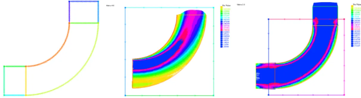
Figure 1: Left: Surfaces of constant pressure for a flow with ν = 10−3, b= 200 in a quarter of a torus
with R = 4, r = 2 discretized on a fixed geometry with the Nedelec edge element for the velocity, peacewise constant pressures and linear continuous deformation. Right: same as left but with a mixte Raviart-Thomas element for the displacement
the RT0− P0− RT0+ P0 element, where n
v is the number of vertices, ne the number of
edges, ntthe number of elements We tested these 3 sets of element on a simple geometry:
a quarter of a torus with a pressure drop imposed from the top horizontal cross section to the right vertical one. The cross section of the torus is a circle of radius 1cm. This circle is extruded on a greater circle of radius 4cm. The pressure drop is 6 cos(πt), b = 200 and ν = 0.001.
The time step is 0.05. The mesh has nv = 1395, nt = 6120, ne= 1336. The computation
is stopped at t = 0.75.
The results are shown on figure 4. On a core [email protected] it takes 17 seconds with the Nedelec-P1−P1element to compute 16 time steps with the characteristic-Galerkin method
for the non-linear terms (see [15]) and 22 seconds with the Nedelec/Raviart-Thomas element (see figure 1).
4 A formulation where the Displacement is Eliminated
Notice that η can be eliminated from (10), giving a formulation which contains u × n = 0: n∂tp = α∂tu + bu (22)
4.1 A Time discretisation
Consider now (19) discretized in time : Z Ω [ρf(um+1− u m δt − u m+1 2 × ∇ × um) · ˆu + µ∇ × um+ 1 2 · ∇ × ˆu −pm+1∇ · ˆu − ˆp∇ · um+ 1 2] + Z ∂Ω pm+1u · n = 0. (23)ˆ We use (22) discretized in time to compute pm+1|
∂Ω and so we consider
Problem 2 Find u, p such that ∀ˆu, ˆp with u and ∂tp given at t = 0,
Z Ω [ρf(um+1− u m δt − u m+1 2 × ∇ × um ) · ˆu + µ∇ × um+ 1 2 · ∇ × ˆu − pm+1∇ · ˆu − ˆp∇ · um+ 1 2] + Z ∂Ω [δtbum+12 + α(um+1− um) + pmn] · ˆu = 0. (24)
Formulation (19) is valid only if ˆu × n = 0. This condition has been removed from (24) to make it symmetric and easy to implement but the consequence is that by working the integrations by parts backward, it is found that this formulation implies (18) and on ∂Ω:
[δtbum+1
2 + α(um+1− um)] · n − (pm+1− pm), ∇ × um+12 × n = 0 (25)
The first condition no longer implies that u × n = 0 and the second condition is like saying that the tangential stress is zero, which means that we match not only the normal components of the fluid and solid normal stress but all the components.
In summary Problem 2 is different from problem 1; both of them have physically sound background but we need to test them numerically to see how different they are.
4.2 Discretization with a Finite Element Method
Let Th be a triangulation with K tetraedra {Tk}K1 with the usual conformity hypotheses;
let Ω := ∪kTk ⊂ R3.
Consider the P2− P1 element built from
Vh = {v ∈ C0(Ω)3 : vi|Tk ∈ P
2, i = 1, 2, 3}
Qh = {q ∈ C0(Ω) : q|Tk ∈ P
1} (26)
We assume that the boundary is made of two part, Σ which is the compliant wall and the input and output sections Γ on which p is given and u × n = 0.
4.3 Discretization of Problem 1
For simplicity we assume that r << R, i.e. α = 1. The momentum equation is also divided by ρf and ν = µ/ρf and b is changed into b/ρf.
A feasible discretization of (20) is to find [um+1, pm+1, ηm+1] ∈ V
h× Qh× Qh with um+1×
n|Γ = 0, ηm+1|Γ= 0 and such that
Z Ω [ˆu · (u m+1− um δt − u m+1 2 × ∇ × um) − pm+1∇ · ˆu − ˆp∇ · um+ 1 2] + Z Ω ν∇ × um+12 · ∇ × ˆu + ε∇ηm+ 1 2 · ∇ˆη] + Z Σ b[ηm+12uˆn− ˆη(um+ 1 2 n − 1 δt(η m+1− ηm)) + 1 ǫ(u m+1 2 × n) · (ˆu × n)] = − Z Γ pΓuˆn, ∀ [ˆu, ˆp, ˆη] ∈ Vh× Qh× Qh with ˆu × n|Γ = 0, ˆη|Γ = 0. (27)
where ε is any small positive parameter.
When Ω is kept fixed, an energy consevation identity is found by choosing ˆu = um+1 2, ˆ p = −pm+1, ˆη = ηm+1 2: Z Ω [u m+12− um2 δt + ν 2|∇u m+1 2 + ∇um+ 1 2 T |2 +ε|∇ηm+12|2] + Z Σ ηm+12 − ηm2 δt +1 ǫ Z Σ |um+12 × n|2 = − Z Γ pΓuˆ m+1 2 n (28)
As for the Navier-Stokes equations, when δt is small enough the problem has a unique solution because of the energy estimate and because of a general inf-sup condition is satisfied with p replaced by [p, η].
4.4 Discretization of Problem 2
A feasible discretization of (24) is to find um+1 ∈ V
h, pm+1 ∈ Qh such that Z Ω [ˆu · (u m+1− um δt − u m+1 2 × ∇ × um) − pm+1∇ · ˆu − ˆp∇ · um+12] + Z Ω ν∇ × um+12 · ∇ × ˆu + Z Σ (um+12bδt + pmn) · ˆu = − Z Γ pΓuˆn ∀ˆu ∈ Vh, ˆp ∈ Qh with ˆu × n|Γ = 0 (29) Notice that um+1× n|
Σ = 0 is implied by the formulation. When Γ is flat that condition
amounts to some component of the velocity being zero which is easy to implement. Notice that the energy equality implies stability only so long a p remains bounded on Σ, which could possibly be derived from (29), but not so obviously:
Z Ω [u m+12− um2 δt + ν|∇ × u m+1 2|2] + Z Σ b|um+12|2δt = − Z Σ pmum+12 n − Z Γ pΓuˆ m+1 2 n (30)
5 Numerical Tests
5.1 Moving the Geometry for Graphic Visualization
The full model requires that Σ be moved at every time step along its normal of a quantity δtum· n. To preserve the triangulation we follow the literature [2] and solve an additional
problem
−∆dm+1 = 0 in Ω, dm+1|Σ = dm+ nδtumn, d m+1|
Γ = 0 (31)
and then move every vertex qj of the triangulation qj → qj+ κd. In theory κ = 1 but for
graphic enhancement it can be adjusted. Note however that (31) is expensive. 5.2 Comparison of the two Methods
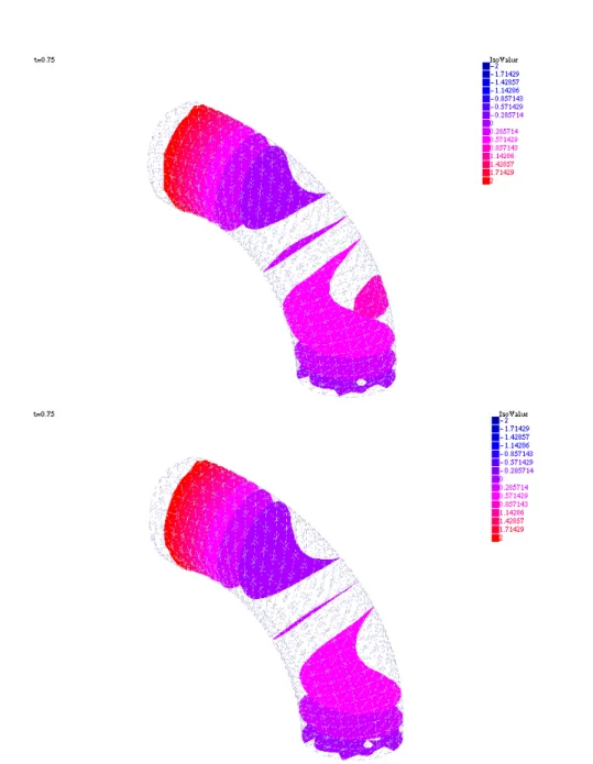
On the problem described earlier both methods give very similar results as shown on figure 2. The geometry is updated for visualisation purpose with a multiplicative factor 100.
The geometry is a section of the aorta obtained from a MRI scan. It has 4991 vertices, giving 19964 degrees of freedom for each linear systems for [um+11 , um+12 , um+13 , pm+1]. The
pressure drop from inflow section on the right to outflow section on the left is pΓR =
6 cos2(πt) and the results are shown at t = 0.8. On the smaller cross sections a pressure
drop equal to pΓR/2 is imposed. Problem 1 and Problem 2 are solved for comparison
with δt = 0.05/π, ν = 0.001, b = 200. Results are shown on figure 3. For Problem 1, the computation took 198” on a macbook pro 15”, 2012, 2.3MHz core i7. For Problem 2 it took 180”. The results are very similar with some difference on the pressure but very little on the velocities.
6 Inflow/outflow Conditions by PML
We end this article with an idea to address the problem of loss of stability due to the creation of reverse flow in unwanted regions because of the boundary conditions on the artificial inflow and out flow sections.
We borrow the idea from the PML literature (see for example [3]) and add to the artery geometry a viscous buffer after Γout where ν = ν1 >> νblood (and similarly before Γin but
we present the idea applied to the outflow section only).
Consider a geometry Ω where the exit section is Γo = {0} × [0, h] in 2D where pressure
is set to p0 while pressure is set to p1 on entry. Assume that we impose a parabolic flow
u = Ky(h − y) at the exit of a viscous buffer L = [−L, 0) × [0, h], i.e. on {−L} × [0, h]. Now we solve the Navier-Stokes equations on Ω ∪ L. The problem is to choose K so that the pressure on the inital outflow boundary Γo is unchanged in the mean, namely
¯
p0 := h−1
R p0dy.
Because at every time step the system to solve is linear we shall adjust K by superposition so that the mean pressure is ¯p0 on Γout. Since, p|Γout ≈ ¯p1 + (¯p2− ¯p1)
K−K1
Figure 2: Left: surface of equal pressure at t = 0.75 computed by solving Problem 1 with P2
− P1
− P1
elements and a penalization of the condition u × n = 0. Right: same as left but with Problem 2 and a P2
− P1
Figure 3: Computation of [u, p] for Problems 1 & 2 for a portion of an oarta (shown upside down). Top: with Problem 1. the pressure is shown at t = 0.8 on the left on a geometry which has changed by η. On the right the third component of the velocity w is shown on the fixed geometry. Bottom: same for Problem 2.
computed with K = K1 and ¯p2 the mean pressure when K = K2, then K = K1+ (K2− K1) ¯ p0− ¯p1 ¯ p2− ¯p1 (32) This requires to solve the linear Stokes-like system at each time step 3 times. We can also add K to the unknowns of the Stokes-like linear system and add RΓoutp = |Γout|p0 to
the equations; we used this second solution in the numerical tests because it is much less computer intensive.
Figure 4: Left: Geometry for the flow with two PLM regions added. Center: the velocity vectors computed without the PML; notice the back flow in the yellow region. Right: the same flow (velocity vectors) computed with the two PML regions. The pressure drop from the two inner boundaries (corresponding to the top and left boundaries of the geometry on the center figure) are the same as in the center figure.
The idea is tested numerically on a quarter of a 2D-torus with radii 0.6 and 1 with ν = 0.002 and a pressure drop equal to cos(t) + cos(3t), t ∈ (0, 25). The PML viscosity is ν1 = 0.2. A PML region is added to both ends of the tube. Results are shown on figure
4.
The results look very different and that is because both computations do not have the same inflow and outflow conditions on the original inflow/outflow boundaries. In one case the pressure is imposed pointwise with u × n = 0, in the PML case the mean pressure is imposed and no conditions are imposed on the velocity but parabolic velocity is imposed on the inflow/outflow of the PML boundaries.
The method will be tested in 3D and reported in a future publication. 7 Conclusion
In this article we have presented problems and solutions encountered with fluid-structure interactions when a middle solution is seeked: neither the full problem with moving geometries because it is too expensive, nor rigid walls because it is not precise enough and it doesn’t give the geometrical deformation.
The solution adopted here is to delay the geometrical deformations to the graphic diplay only. But in doing so we have to work with the Navier-Stokes equations with unusual boundary conditons which require unusual finite element discretizations.
For these intermediary problems we have shown that it is important to preserve energy. Furthermore we can choose either to match exactly the normal component of the solid and fluid normal stress tensor or to match approximately the 3 componenets of the normal stresses by relaxing slightly the no slip condition.
In all cases the problem of back flows in the pulsating cases remains. We have suggested a possible solution and made some preliminary tests.
Acknowledgement
All computations were done with freefem++ [10] (www.freefem.org/ff++). We are grate-ful to F. Hecht for his help.
REFERENCES
[1] D. Boffi, L. Gastaldi, A FEM for the immersed boundary method, Comput. Struct. 81(2003),491-501
[2] S. Deparis, M.A. Fernandez and L. Formaggia, Acceleration of a Fixed Point Algorithm for Fluid-Structure Interaction using Transpiration Conditions. ESAIM:M2AN Vol.37,No 4,2003, 601-616
[3] Fang Q. Hu, X.D. Li, D.K. Lin. Absorbing boundary conditions for nonlinear Euler and Navier-Stokes equations based on the perfectly matched layer technique. J. of Comp. Physics 227 (2008) 4398-4424.
[4] M. Fernandez, Incremental displacement-correction schemes for incompressible fluid-structure interaction. Numer. Math. (2013) 123:21-65.
[5] L. Formaggia, J.F. Gerbeau, F. Nobile, A. Quarteroni, On the coupling of 3D and 1D Navier-Stokes equations for flow problems in compliant vessels. Comput. Methods Appl. Mech.Engrg.191(2001)561-582.
[6] L. Formaggia, A. Quarteroni, A. Veneziani eds. Cardiovasuclar Mathematics. Springer MS&A series 2009.
[7] V. Girault, Incompressible Finite Element Methods for Navier-Stokes Equations with Nonstandard Boundary Conditions in R3. Math. of Comp. Vol 51, No 183, pp 55-74,
July 1988.
[8] O. Gonzalez, J.C. Simo On the Stability of Symplectic and Energy-Momentum Algorithms for Nonlinear Hamiltonian Systems with Symmetry. Comput. Methods Appl. Mech. Engrg. 134 (1996) 197-222.
[9] O. Gonzalez Exact energy and momentum conserving algorithms for general mod-els in nonlinear elasticity. Comput. Methods Appl. Mech. Engrg. 190 (2000) 1763-1783
[10] F. Hecht New development in freefem++,nJ. Numer. Math. vol 20, no 3-4, pp 251–265 (2012).
[11] P. Le Tallec Fluid structure interaction with large structural displacements. Com-put. Methods Appl. Mech. Engrg 190, 3039-3067. 2001.
[12] F. Nobile and C. Vergana, an effective fluid-structure interaction formulation for vascular dynamics by generalized robin conditions. SIAM J. Sci. Comp. Vol. 30, No. 2, pp. 731-763 (2008)
[14] C. Peskin and D. McQueen, A three dimensional computational method for blood flow in the hearth-I. Immersed elastic fibers in a viscous incompressible fluid, J. Comput. Phys. 81 (1989) 372-405.
[15] K.G. Pichon and O. Pironneau
[16] O. Pironneau. Finite Element Methods for Fluids, Wiley 1989.
[17] O. Pironneau. Conditions aux limites sur la pression pour les ´equations de Stokes et de Navier-Stokes. C. R. Acad. Sci. Paris S´er. I Math., 303(9):403–406, 1986. [18] M. Thiriet, Biomathematical and Biomechanical Modeling of the Circulatory and
Ventilatory Systems. Vol 2: Control of Cell Fate in the Circulatory and Ventilatory Systems. Springer Math& Biological Modeling 2011.
[19] F. Usabiaga, J. Bell, R. Buscalioni, A. Donev, T. Fai, B. Griffith, and C. Peskin. Staggered schemes for fluctuating hydrodynamics. Multiscale Model Sim. 10:1369-1408, 2012.
[20] I. Vignon-Clementel , A. Figueroa, K. Jansen, C.A. Taylor Outflow boundary conditions for three-dimensional finite element modeling of blood flow and pressure in arteries. Comput. Methods Appl. Mech. Engrg. 195 (2006) 3776-3796.

![Figure 3: Computation of [u, p] for Problems 1 & 2 for a portion of an oarta (shown upside down)](https://thumb-eu.123doks.com/thumbv2/123doknet/14604428.544407/12.918.130.770.263.897/figure-computation-problems-amp-portion-oarta-shown-upside.webp)