Bayesian design of experiments for complex chemical systems

-t

Bayesian Design of Experiments

for Complex Chemical Systems

by

Kenneth T. Hu

B.S., Carnegie Mellon University (2006)

M.S.CEP, Massachusetts Institute of Technology (2010)

Submitted to the Department of Chemical Engineering

in partial fulfillment of the requirements for the degree of

Doctor of Philosophy in Chemical Engineering

at the

MASSACHUSETTS INSTITUTE OF TECHNOLOGY

June 2011

JUN 13 2011

LIBRARIES

ARCHIVES

@

Massachusetts Institute of Technology 2011. All rights reserved.

A uthor ...

-...

Department of Chemical Engineering

March 25, 2011

C ertified by ...

...

Gregory McRae

Hoyt C. Hottel Professor of Chemical Engineering

Thesis Supervisor

A ccepted by ...

William M. Deen

Professor of Chemical Engineering

Chairman, Committee for Graduate Students

Bayesian Design of Experiments

for Complex Chemical Systems

by

Kenneth T. Hu

Submitted to the Department of Chemical Engineering on March 25, 2011, in partial fulfillment of the

requirements for the degree of

Doctor of Philosophy in Chemical Engineering

Abstract

Engineering design work relies on the ability to predict system performance. A great deal of effort is spent producing models that incorporate knowledge of the underlying physics and chemistry in order to understand the relationship between system inputs and responses. Although models can provide great insight into the behavior of the system, actual design decisions cannot be made based on predictions alone. In order to make properly informed decisions, it is critical to understand uncertainty. Otherwise, there cannot be a quantitative assessment of which predictions are reliable and which inputs are most significant. To address this issue, a new design method is required that can quantify the complex sources of uncertainty that influence model predictions and the corresponding engineering decisions.

Design of experiments is traditionally defined as a structured procedure to gather information. This thesis reframes design of experiments as a problem of quantifying and managing uncertainties. The process of designing experimental studies is treated as a statistical decision problem using Bayesian methods. This perspective follows from the realization that the primary role of engineering experiments is not only to gain knowledge but to gather the necessary information to make future design decisions. To do this, experiments must be designed to reduce the uncertainties relevant to the future decision. The necessary components are: a model of the system, a model of the observations taken from the system, and an understanding of the sources of uncertainty that impact the system.

While the Bayesian approach has previously been attempted in various fields including Chem-ical Engineering the true benefit has been obscured by the use of linear system models, simplified descriptions of uncertainty, and the lack of emphasis on the decision theory framework. With the recent development of techniques for Bayesian statistics and uncertainty quantification, including Markov Chain Monte Carlo, Polynomial Chaos Expansions, and a prior sampling formulation for computing utility functions, such simplifications are no longer necessary. In this work, these meth-ods have been integrated into the decision theory framework to allow the application of Bayesian Designs to more complex systems.

The benefits of the Bayesian approach to design of experiments are demonstrated on three sys-tems: an air mill classifier, a network of chemical reactions, and a process simulation based on unit operations. These case studies quantify the impact of rigorous modeling of uncertainty in terms of reduced number of experiments as compared to the currently used Classical Design methods. Fewer experiments translate to less time and resources spent, while reducing the important

uncer-tainties relevant to decision makers. In an industrial setting, this represents real world benefits for large research projects in reducing development costs and time-to-market. Besides identifying the best experiments, the Bayesian approach also allows a prediction of the value of experimental data which is crucial in the decision making process. Finally, this work demonstrates the flexibility of the decision theory framework and the feasibility of Bayesian Design of Experiments for the complex process models commonly found in the field of Chemical Engineering.

Thesis Supervisor: Gregory McRae

Acknowledgments

It's hard to believe that I'm finally leaving the McRae lab. It has been five years of both excitement and frustration but I can honestly say I've had a wonderful time at MIT. I want to thank the many remarkable people who have shaped my life here.

First I thank my advisor, Gregory McRae. He has helped me develop my analytical skills and given me the perspective to take on any challenges. I have benefited from the advice and knowledge he has passed on and learned to find my own way. I want to thank him for giving me guidance and life lessons when I needed them and for not counting vacation days. Thanks to the rest of the McRae lab - Arman Haidari, Bo Gong, Kunle Adeyeme, Ingrid Berkelmans, Mihai Anton, Alex Lewis, Chuang-Chuang Lee and Carolyn Seto for the helpful discussions and inspiration, and Joan Chisholm for always listening and putting up with us.

My thesis committee, Professor William Green and Professor Youssef Marzouk, have given me

plenty of advice for navigating the academic world and invaluable technical help. Also a special thanks to Professor Marzouk and the UQ reading group, in particular Xun Huan, who have all helped me gain a broader appreciation for the work I've done.

I acknowledge the support of Eni S.p.A. who have funded my Ph.D. work. Roberto Bagatin, Ernesto Rocarro, Letizia Bua, Irene Rapone, and Fabio Oldani, all provided help with my thesis work and hosted me in Novara. It was a great experience and I hope to return someday.

Beyond the basement, I want to thank all my friends and classmates, the Mooseheads, and the Landau IM teams. I have so many treasured memories and I will miss being here with all of you. I'm also glad I found the AJJ club. Remember, the beatings will continue until morale improves.

To Lauren: the past few years would have been incomplete without you. I needed your encour-agement, your smiles, and the regular doses of culture more than I could have known.

To my family: your guidance has taught me who I want to be and your support has helped me achieve all that I have. Thank you.

Contents

1 The Future of Experimental Design 19

1.1 The Experimental Process and Experimental Design . . . 20

1.2 The Bayesian Approach to Design of Experiments . . . 20

1.3 Motivating Study . . . 21

1.4 Thesis Structure . . . 22

1.5 Thesis Contributions . . . 22

2 Background Theory 25 2.1 Uncertainty and Modeling . . . . 25

2.2 Probability Theory . . . . 29

2.3 Information Theory . . . . 40

2.4 Decision Theory . . . . 43

2.5 Optimization . . . . 49

3 Methods for Uncertainty Quantification 55 3.1 Examples . . . . 55

3.2 Formulating an Uncertainty Quantification Problem . . . . 59

3.3 Uncertainty Quantification with Monte Carlo . . . . 63

3.4 Polynomial Chaos Expansions . . . . 69

3.5 Uncertainty Quantification with Polynomial Chaos Expansions . . . . 90

3.6 Projection Methods . . . 101

3.7 Collocation Methods . . . 114

3.9 Summary ...

4 Classical Design of Experiments

4.1 The Current State of Experimental Design . 4.2 History of Design of Experiments . . . . 4.3 Classical Design Heuristics . . . .

. 123

125

. 125 . 126 . 126

5 Model Based Design of Experiments 129

5.1 Decision Theory for Design of Experiments . . . 129

5.2 Illustrative Examples of Model Uncertainty . . . 135

5.3 Optimal Design of Experiments . . . 143

5.4 Bayesian Design of Experiments . . . 146

6 Bayesian Methods for Estimation and Design 153 6.1 Bayes' Theorem . . . 153

6.2 Bayesian Parameter Estimation . . . 159

6.3 Markov Chain Monte Carlo . . . 161

6.4 Prior Sampling Formulation . . . 165

6.5 Polynomial Chaos Expansion Based Surrogate Models . . . 172

7 Design of Experiments Examples 7.1 Sequential Reactions in a Batch Reactor 7.2 Discrimination Between Linear Models . 7.3 Conclusion . . . . 8 Study 1: Air Mill and Classifier 8.1 Background and Previous Work ... 8.2 Classical Design of Experiments . . . . . 8.3 Bayesian Designs - Building Models . . 8.4 Bayesian Designs - Procedure . . . . 8.5 Results . . . . 8.6 Discussion . . . . 8.7 Conclusions . . . . 175 175 181 186 189 . . . 189 . . . 192 . . . 195 . . . 205 . . . 206 . . . 210 . . . 212

9 Study 2: Reaction with Uncertain Stoichiometry 213

9.1 Background ... ... 213

9.2 M odels . . . 214

9.3 Study G oals . . . 218

9.4 Analysis of Prior Knowledge . . . 219

9.5 M ethods . . . 223

9.6 R esults . . . 226

9.7 Conclusion and Discussion . . . 231

10 Study 3: Biomass-to-Liquids Process 233 10.1 The Biomass-to-Liquids Process . . . 233

10.2 Fischer-Tropsch Flowsheet . . . 234

10.3 Uncertainty Analysis with Polynomial Chaos Expansions . . . 236

10.4 Design of Experiments . . . 240

10.5 R esults . . . 242

10.6 Conclusion and Discussion . . . 245

11 Conclusions 247 11.1 A Focus on Uncertainty . . . 247

11.2 Case Studies . . . 248

11.3 Using Appropriate Methods . . . 249

11.4 Advantages of Bayesian Designs . . . 250

12 Thesis Contributions 251 12.1 Synthesis of Methods . . . 251

12.2 Dem onstration . . . 252

13 Directions for Future Work 253 13.1 Sensitivity of Results . . . 253

13.2 Risk Informed Decision Making . . . 254

13.3 Direct Comparison to Other Model Based Approaches . . . 256

A Probability, Statistics, and Estimation 259

A.1 Full Definition of Random Variables ... ... 259

A.2 Important Details about Probability Theory . . . 261

A.3 Estimation Theory . . . 263

B Information Theory 267 B.1 Fisher Information . . . 267

B.2 Connections . . . 268

B.3 Interpretation . . . 268

B.4 Cramer-Rao Bound . . . 269

B.5 Optimal Designs, Fisher Information and the Cramer-Rao Bound . . . 270

C Design of Experiments Theory 281 C.1 General Principles of Classical Approaches . . . 281

C.2 Sum m ary . . . 283

C.3 The Role of Experimental Design . . . 283

C.4 Organizing Experimental Studies . . . 283

C.5 Prior Knowledge . . . 285

C.6 Overview . . . 287

D Utility Functions and the Prior Sampling Formulation 291 D.1 Prior Sampling Formulation of Information Metrics for Design of Experiments . . . . 291

D.2 Utility Functions for Model Discrimination . . . 298

D.3 Comparing Utility Functions for Parameter Estimation . . . 307

E Model Based Experimental Designs 311

List of Figures

1-1 Flowchart of the experimental study process . . . . 1-2 The Experimental Process and Components of Decision Theory

The Uncertain Radius of a Ball Bearing . . . . Visual Descriptions of Uncertainty Using Probability Theory Convergence of the Sum of Uniform Random Variables . . . .

Convergence of the Sum of Exponential Random Variables . . Sum of Eight Random Variables . . . . The Ratio of Two Gaussian Random Variables . . . . The variance statistic . . . . Decision Tree for Choosing How to Commute to Work .

Complete Decision Tree for Example 6 . . . . Distributions of Utility Due to the Uncertain Consequences of

. . . . 31 . . . . 34 . . . . 36 . . . . 37 . . . . 38 . . . . 39 . . . . 41 . . . . 45 . . . . 47 Two Actions . . . . . 49 2-1 2-2 2-3 2-4 2-5 2-6 2-7 2-8 2-9 2-10 3-1 3-2 3-3 3-4 3-5 3-6 3-7 3-8 3-9

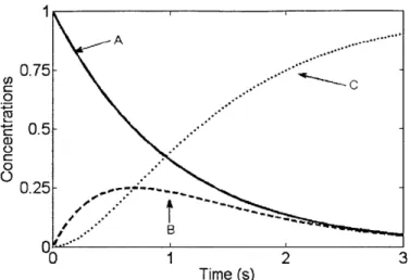
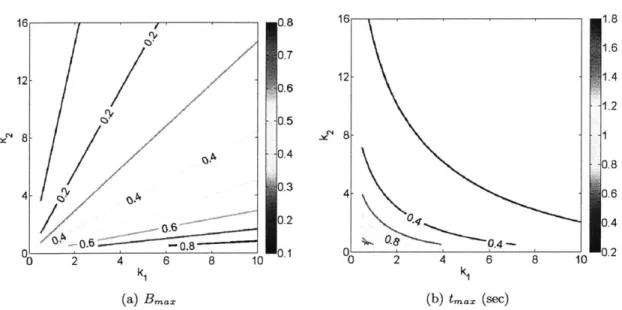
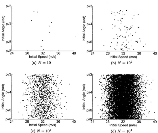
Example 7 - Target Practice with Uncertain Cannonball Trajectory . . . . Example 8 - Sequential Isomerization Reactions of Pentane . . . . Concentration Profiles versus Time in a Sequential Reaction . . . . Maximum Concentration of Species B and Corresponding Time in a Sequential Re-action ... ... ... . .... ... ... ...

Procedure for Solving Uncertainty Quantification Problems . . . . The Joint Probability Density Function of Two Uncertain Parameters . . . . Propagation of Uncertain Parameters Through a Process Model . . . . Sampling Uncertain Parameters from Example 7 using Monte Carlo . . . . Potential Cannonball Trajectories due to Uncertain Initial Conditions . . . .

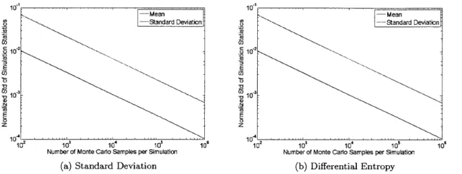
3-10 Cannonball Impact Location Uncertainty Computed by Monte Carlo . . . . 66

3-11 Verification of the Monte Carlo Solution . . . . 68

3-12 Another Verification of the Monte Carlo Solution . . . . 69

3-13 Fourier Series with Increasing Number of Terms . . . . 71

3-14 Polynomial Chaos Expansion of an Uncertain Kinetic Parameter . . . . 73

3-15 Visualizing a Lognormal Polynomial Chaos Expansion . . . . 85

3-16 Visualizing a Truncated Exponential Polynomial Chaos Expansion . . . . 87

3-17 Uncertainty Quantification with Polynomial Chaos Expansions . . . . 90

3-18 Polynomial Chaos Expansion Coefficients Solved using the Projection Method with M onte Carlo . . . 109

3-19 Gaussian Quadrature Points . . . 112

3-20 Polynomial Chaos Expansion Coefficients Solved using Probabilistic Collocation . . . 120

3-21 Uncertainty Profile of Species B in a Sequential Reaction . . . 120

5-1 Comparison of Model Based Approaches to Design of Experiments . . . 135

5-2 First-order, Linear System with Parametric Uncertainty . . . 137

5-3 First-order Linear System with Parametric and Observation Uncertainty . . . 138

5-4 Offset Linear System Model . . . 139

5-5 Second-order, Linear System with Gaussian Parametric and Objservation Uncertainties 140 5-6 Proportional Observation Model Uncertainty . . . 141

5-7 A Nonlinear System Model . . . 142

5-8 Effect of Linearization on Model Output Uncertainty . . . 143

5-9 Information Flow During the Experimental Process . . . 147

6-1 Monty Hall Problem Described with a Decision Tree . . . 157

6-2 Bayesian Parameter Estimation to Determine the Bias of a Coin . . . 160

6-3 Markov Chain Monte Carlo Solution to Parameter Estimation from Example 23 . . 164

7-1 Prior Predictive Density of Species B . . . 177

7-2 Results from Different Datasets . . . 180

7-3 Sequential Reactions Design of Experiments Results . . . 180

Prior Model Output Densities . . . . Hierarchical Model Output Density . . . . Objective Functions for Optimal Designs for Model Discrimination

. . . 183 . . . 183 . . . 185 7-5 7-6 7-7 8-1 8-2 8-3 8-4 8-5 8-6 8-7 8-8 8-9 8-10 8-11 8-12 8-13 9-1 9-2 9-3 9-4 9-5 9-6 9-7 9-8 9-9 9-10 9-11 9-12 9-13 An Air M ill Classifier ... Flowsheet of an air mill and classifier . . . . Pilot and Production Scale Comparison . . . . Particle Size Cumulative Distribution in the Feed Stream . . . . Fluidization Velocity and Particle Radius . . . . Diagram of the Classifier Unit . . . . Particle Release from Classifier . . . . Particle Size Distribution of Product . . . . Classical Screen Study compared with Model Based Experimental Design Posterior Distributions from Bayesian Parameter Estimation... Pilot Scale Results . . . . Production Scale Results . . . . Production Scale Model Output X9o . . . . Nominal Concentration Profiles at Two Temperatures . . . . Prior Parameter Knowledge . . . . Uncertainty Analysis of Uncertain Stoichiometry System Model at 300 K . Uncertainty Analysis of Uncertain Stoichiometry System Model at 700 K . Global Sensitivities of Model Output B . . . . Global Sensitivities of Model Output C . . . . Global Sensitivities of Data Predictions B . . . . Global Sensitivities of Data Predictions C . . . . Classical Designs for Uncertain Stoichiometry Study . . . . Uncertain Stoichiometry Study Results - Estimating All Parameters . . . Uncertain Stoichiometry Study Results -Estimating p . . . . Representative Prior and Posterior Marginal Parameter Densities - Bayesian Design 229 Uncertain Stoichiometry Study Results -Estimating A and /3 . . . 229

. . . 190 . . . 190 . . . 194 . . . 199 . . . 201 . . . 202 . . . 203 . . . 203 . . . 207 . . . 207 . . . 208 . . . 209 . . . 210 . . . 215 . . . 217 . . . 219 . . . 220 . . . 221 . . . 221 . . . 222 . . . 222 . . . 224 . . . 226 . . . 228

9-14 Uncertain Stoichiometry Study Results -Estimating Ao . . . .

10-1 Flowsheet of the Fischer-Tropsch process and product separations . . .

10-2 Prior Parameter Densities . . . .

10-3 Uncertainty in the Economic Metrics with Four Uncertain Parameters

10-4 Uncertainty in the Product Streams with Four Uncertain Parameters .

10-5 Surrogate Model for Fisher-Tropsch Flowsheet . . . . 10-6 Fischer-Tropsch Study Results . . . . 13-1 The Stage-Gate Decision Process . . . . 13-2 Risk Informed Decision Making Example . . . .

. . . 231 . . . 235 . . . 237 . . . 238 . . . 239 . . . 241 . . . 244 . . . 254 . . . 255

List of Tables

2.1 Table of Consequences and Associated Utilities . . . 47

6.1 Maximum Entropy Distributions . . . 155

7.1 Bayesian Optimal Designs Model Discrimination . . . 186

8.1 Approximating Gaussian Distributions of the Model Parameters . . . 204

8.2 Initial Ranges of Process Variables . . . 204

8.3 Prior distributions of model parameters used for parameter estimation . . . 205

8.4 Parameters Used for Scale Up of Equipment . . . 209

8.5 Variable Costs of Two Experimental Studies . . . 211

9.1 Classical Design Points (time in sec, Temp in K) . . . 224

9.2 Bayesian Optimal Designs for Estimating All Parameters . . . 227

9.3 Bayesian Optimal Designs for Estimating A and

#

List of Examples

Example 1: Modeling an Uncertain Quantity ... 30

Example 2: Visual Descriptions of Uncertainty Using Probability Theory ... 33

Example 3: The Central Limit Theorem ... 35

Example 4: When the Central Limit Theorem Does Not Apply ... 35

Example 5: Gaussian Parametric Uncertainties in a Linear Model ... 38

Example 6: Commuting in the Rain ... 44

Ex. 6a: Formal Statement and Solution ... 45

Exam ple 7: Target Practice ... 55

Example 8: Sequential Chemical Reactions ... 56

Ex. 7a: Formulating an Uncertainty Quantification Problem ... 61

Ex. 7b: Target Practice Input Uncertainty ... 65

Ex. 7c: Target Practice Verification ... 67

Exam ple 9: Fourier Series ... 70

Ex. 8a: Sequential Reactions: Polynomial Chaos Expansion of parameter K1 ... . . . .72

Exam ple 10: The M ulti-index ... 75

Example 11: Hermite Polynomials ... 76

Example 12: Legendre Polynomials ... 77

Example 13: Gram-Schmidt Orthogonalization ... 79

Exam ple 14: Basis Functionals ... 81

Example 15: Polynomial Chaos Expansion of a Lognormal Random Variable ... 84

Ex. 8b: Generating a Polynomial Chaos Expansion from Statistics ... 87

Ex. 7d: Using Polynomial Chaos Expansions for Uncertainty Quantification ... 92

Ex. 7e: Target Practice Uncertainty Quantification with Projection Methods ... 104

Ex. 7f: Projection Method using Monte Carlo ... 108

Ex. 7g: Projection Method using Gaussian Quadrature ... 109

Ex. 7h: Probabilistic Collocation M ethod ... 117

Ex. 8d: Solved with the Probabilistic Collocation Method ... 119

Example 16: Uncertainty Quantification Methods Comparison in One-Dimension ... 122

Example 17: First-order, Linear System with Gaussian Uncertainties ... 136

Example 18: Offset, First-order, Linear System with Gaussian Uncertainties ... 137

Example 19: Second-order, Linear System with Gaussian Uncertainties ... 138

Example 20: Second-order, Linear System with Proportional Observation Uncertainty ... 140

Example 21: Nonlinear System M odel ... 141

Example 22: The M onty Hall Problem ... 156

Exam ple 23: A Biased Coin ... 159

Ex. 23a: Markov Chain Monte Carlo Solution ... 163

Chapter 1

The Future of Experimental Design

We learn about systems by building, testing, and observing. This is true whether the system is a machine, social group, or computer simulation. Experiments are one way we can control the way information is gathered from a system. Examples include measurements or observations, surveys of experts, or the evaluation of the computer model. The common connection is that information is revealed by running the experiment.

Design of experiments is the exercise of selecting specific experiments in order to gather relevant information. If infinite resources and time were available then we would not be concerned with experimental design. We could simply run experiments until we obtain useful results. In reality, experiments must be selected intelligently in order to collect information in an efficient and effective manner. Unfortunately, it is difficult to know exactly what experiments should be used and how many are required - each study has unique goals and therefore requires different information.

In engineering fields we have a wealth of knowledge about the systems we use. We understand many of the underlying principles that dictate system performance or at least have empirical obser-vations that can describe the system. It is commonplace and even required to use this knowledge for process design and optimization but it is rarely seen in the design of experimental studies. This represents a great opportunity because incorporating this knowledge into the design of experiments process can greatly reduce the required number of experiments - saving time, resources, and money.

The goal of this thesis is to change the way information is gathered by focusing on the treatment of uncertainty. Much attention has been paid to improving process modeling, numerical methods, and optimization. The treatment of uncertainty during the design process often overlooked. The

vast majority of experiments being done today either use Classical Design of Experiments or skip the explicit design of experiments step altogether. These experiments are still guided by the expertise of the researcher, but prior knowledge, models, and uncertainty do not explicitly influence the design. This results in the inefficient use of resources and time.

1.1

The Experimental Process and Experimental Design

To better understand how to design experiments, we first examine how an experimental study is carried out. In a study, design, experiments, and analysis are iterated to gather evidence until the goals are reached or resources are exhausted. This is illustrated in Figure 1-1.

Prior Design of Col lect 1 Analyze Assess

TKnowlede Experiments

Data Data Goals

Goals Not Met

Goals Met

Figure 1-1: Flowchart of the experimental study process showing the role of design of experiments

Ideally, we could somehow determine how useful every possible experiment will be and run only the most useful. Unfortunately, this information only after the experiments are run and data is analyzed. Therefore, more practical design of experiment approaches have been developed. Design of experiments approaches are used to determine the best experiments to run, however, it is important to understand that the root of this problem is estimating the usefulness of a future experiment. Each design of experiments approach accomplishes this in a different way; this thesis focuses on the Bayesian approach.

1.2

The Bayesian Approach to Design of Experiments

In order to incorporate all the prior knowledge and treat uncertainties, we take a general ap-proach that models the entire experimental process. The design step is posed as a decision problem, where the engineer must select the best experiment out of all possible experiments. The framework from decision theory organizes and connects various ideas: how to describe the process knowledge and uncertainty, value information, and use optimization methods. This is called the Bayesian

approach or simply Bayesian Designs because many of the methods rely on Bayes' Theorem (See Chapter 6 in particular). These connections are illustrated in Figure 1-2.

Prior Design of Collect Analyze Assess

Knowledge

H

H

Theory Quantification Theory

Figure 1-2: The steps in the experimental process can be matched to components of decision theory

Applications in the pharmaceutical and energy industries will serve as initial case studies, how-ever, the techniques illustrated here can be applied to any field and any system. Examples include the design of experiments to characterize equipment, improve system performance, compare models of a system, or even compare two technologies. The ideas are also applicable to other design work such as process design and optimization.

1.3

Motivating Study

The pharmaceutical industry aptly demonstrates the impact of experimental design. Pharma-ceutical companies face two critical challenges: lengthy product development times and process variation. The first is driven by economic concerns - the first product in the market captures and retains a disproportionate amount of the market share, even if a superior product is introduced later. The second is due to government regulation of drug quality. The root cause of both product development times and variability in product quality is the difficulty of gathering useful informa-tion. Before a drug can be sold, a reliable and consistent manufacturing process must be designed, built, and validated. Each step takes experiments and each experiment costs resources and time.

The case study which motivated this work was an experimental project carried out by an industrial partner. They had used Classical Design of Experiments to run four studies for the scale up of a mechanical separation process. Using classical statistical methods and scale up procedures, they developed a model for the production scale equipment that did not accurately predict the true performance. As a result, an additional study was required which increased the time and money spent.

We will examine why this scale up failed and how the experiments could be improved using Bayesian approach to Design of Experiments in Chapter 8.

1.4

Thesis Structure

The building blocks required for decision theory are introduced in Chapters 2, including proba-bility theory, uncertainty, information theory, statistic/ estimation theory, and optimization. More detailed discussion and related topics are also included in the Appendices.

After the background chapters, the various approaches to design of experiments are described in Chapters 4 and 5. The relationships between experimental studies and decision theory shown in Figure 1-2 are emphasized, focusing on the treatment of uncertainty and current process knowledge. The methodologies used in this work are then detailed in Chapter 3: Methods for Uncertainty Quantification, and Chapter 6: Bayesian Methods for Estimation and Design. Finally several examples and case studies are used to showcase the methods and design of experiments framework in Chapters 7 through 10, followed by the conclusions and discussion.

1.5

Thesis Contributions

This thesis provides a substantially different perspective on design work than traditional Chem-ical Engineering Process Systems Engineering methods. The focuses is on uncertainty and decision theory rather than optimization and modeling. This perspective follows from the realization that experiments are not always carried out for gaining knowledge. The true goal is to gather the neces-sary information to make an informed decision. The framework provided in this work gives a clearer picture of the important factors that affect the system and the impact on the future decisions.

The first contribution is the synthesis of the ideas and methodology for properly treating uncer-tainty for design of experiments on chemical engineering systems. While the Bayesian approach has been previously attempted in various fields including chemical engineering [29, 28, 62, 63], the true benefit has been obscured by the use of linear system models, simplified descriptions of uncertainty, and de-emphasis of the decision theory framework. In this work, no simplifying assumptions are taken and the decision theory framework is followed strictly. This allows a quantitative assessment of the decision making benefits gained by properly treating uncertainty. The methods required in-clude: Bayesian probabilistic modeling of uncertainty, use of prior knowledge, use of non-Gaussian distributions and corresponding Information Theory metrics, Markov Chain Monte Carlo methods, and Polynomial Chaos Expansions. Many of these techniques have not previously been applied to

the design of experiments.

The second contribution of this thesis is the application to common chemical engineering systems including chemical kinetics models, a mechanical separations unit, and a process flowsheet. By applying these methods to practical chemical engineering systems the benefits of the Bayesian Design of Experiments approach over the commonly used Classical Designs approach are clearly established.

Chapter 2

Background Theory

This chapter presents the required background theory at the level necessary to understand the remainder of the thesis. Section 2.1 gives a definition for uncertainty and introduces the necessary supporting concepts. Then Sections 2.2 and 2.3 provide the background on probability, statistics, and information theory that provide the basis for Bayesian methods. Finally, Section 2.4 ties all the concepts together to describe the framework used for design of experiments and Section 2.5 discusses the optimization tools that are used in this thesis. Chapters 3 and 6 contain additional details of the most important topics.

2.1

Uncertainty and Modeling

Uncertainty describes the state of imperfect knowledge. For example, the state of a physical system at any instant is well defined and certain but our knowledge about the system is quite uncertain. It is impossible to exactly know the system states because we know only what our instruments and observations tell us. Decisions are often made with incomplete knowledge - we never have enough information about the system to know for sure which decision is best. Therefore it is critical to understand how much knowledge we have and how to improve that knowledge through experiments. In this section, we will discuss the significance, modeling, and quantification of uncertainty and information.

2.1.1

Modeling Uncertainty

A system model relates the system inputs, outputs, states, and parameters to one another. The

model is a mathematical representation of the knowledge we have of the system. Using these models helps engineers understand which inputs, states, or parameters have an impact on the outputs. Since our knowledge is often incomplete, all these quantities have some degree of uncertainty; there can be uncertainty in the physical basis of the model, the mathematical representation, the model parameters, etc. The uncertainty impacts the validity of the model and the ability to make decisions based on the model. Before relying on model predictions for design work, engineers must first have a sense of the quality or the uncertainty of those predictions. We need to be able to relate uncertainty the inputs, states, parameters, etc. to the uncertainty in the outputs and measurable variables.

Still, uncertainty is a vague and subjective concept. Given different levels of understanding and knowledge, two observers of the same event may have different amounts of uncertainty. This presents enormous problems for modeling. To address this issue, uncertainty must be represented in a way that is consistent between observers but still have physical meaning.

2.1.2

Uncertainty and Probability Theory

There are several tools that have been used to characterize uncertainty [65, 18, 19], but here we will use probability theory. Probability theory is mathematically rigorous and provides the neces-sary consistency. For example, although two people can disagree over what probability of a future event, they must agree on the meaning of that probability. In addition, probability is a natural concept to apply to physical systems. While other methods also share these properties, probability theory is an appropriate and widely accepted tool for treating uncertainty in engineering systems. This is sometimes called a Bayesian perspective of uncertainty, in which uncertain quantities are represented by Random Variables. See the books Understanding Uncertainty by David Lindley [51] and Probability Theory by Jaynes [43] for more discussion.

When applying probability theory to engineering systems, we narrow our scope to parametric uncertainties. In these situations we are most interested in true values or optimal values of param-eters. Unfortunately, we are uncertain what these values are. Rather than describing a fixed value and assuming it is the true value, we use probability theory to describe the the uncertain knowledge

of the true value. The key point is that this is modeling our understanding of the parameter, not the parameter - which has a fixed true value.

Statistics and Probability in Engineering

Statistics are used to describe past observations and probability theory to predict future events. Observations of a system always have some variability which is described by a statistical model. These models are then used to estimate parameters and finally to predict future observations. In terms of uncertainty, observations allow us to make inferences about the uncertain state of the system. Using our imperfect knowledge of the system, we can imperfectly estimate the unknown parameters. Using the parameters and the model, we can determine the uncertainty in the model

outputs.

Although there is a great deal in common between the classical model development strategy and our current uncertainty framework, there is one major distinction. The classical approach always assumes that uncertainties can be described by Gaussian probability distributions. The Gaussian distribution is useful because it is remarkably simple to define and manipulate, yet it describes naturally varying processes well. Unfortunately, there are many instances where the Gaussian distribution is inappropriate. To be treated accurately, uncertainty must be described with more fidelity so we will use the entire probability density function. Many commonly used statistical techniques cannot treat non-Gaussian distributions, so we will need to develop more flexible methods. These issues will be discussed further in Section 2.2.

2.1.3 Sources of Uncertainty

There are countless sources of uncertainty when modeling a complex system. To attempt to un-derstand them, they are placed in two categories as modified from a report by the Intergovernmental Panel on Climate Change [59] and an article by Draper [19].

Data Observations

Data can never be treated as a true measurement of the system because the measurement tools are imperfect. There is some uncertain discrepancy between the observations and the true system state. What engineers and scientists strive for is to keep the uncertainty low enough so that the

observation conveys useful information about the system. To model this, we must understand the sources of uncertainty, including but not limited to: random fluctuations in the measurement equipment, influences from factors outside the system, incorrect interpretation of the observation, and observation of the wrong signal. The great difficult with modeling these sources is that they are often unknown and undetectable. As discussed below, these are typically all lumped together along with terms which do not belong.

Modeling

It is an unfortunate fact that models are never completely correct. The physical world has so many factors which influence system performance that a model cannot capture them all. We must accept this fact and simply try to understand how this affects our confidence in the model. This is called the model output uncertainty.

First of all, the model structure is incorrect. Even models built on physical principles will either be missing terms or have the wrong mathematical representation. This is notoriously difficult to detect, much less model, because it is convoluted with other sources of uncertainty. For this reason, model inadequacy is often lumped into the observation uncertainty because the unexplained variations in the model output are mistaken for observation errors. There are other approaches treating model inadequacy [47] which are not explored here.

Secondly, there is uncertainty associated with the numerical computation of model outputs. This is assumed to be negligible throughout this work. This is a safe assumption, as models should always be validated and verified.

Lastly, there is parametric uncertainty. The parameters have physical meaning and are therefore assumed to have a true value, which remains unknown to us. By representing our knowledge of these parameters with Random Variables, we introduce uncertainty into the system model. This is the only source of model uncertainty which is treated rigorously here.

The Quantification of Uncertainty

After lumping many sources of uncertainty together we are left with two main sources: ob-servations and model parameters. Uncertainty quantification is the analysis of the impact these uncertainties have on the model outputs. Uncertainty refers to the probability density function of

the model outputs, while sensitivity is the contribution or relative contribution of a single param-eter to the overall model output uncertainty. Methods for uncertainty quantification are discussed in Chapter 3.

2.1.4

Recap

Now that the ideas are in place to define, model, and quantify uncertainty we return to give an engineering perspective. When we attempt to quantify the uncertainty in a model, the purpose is typically to gain insight into a design problem. In a more general sense, uncertainty analysis helps to make decisions. To show how this is done, some background is required on the various tools that come together to solve decision problems.

2.2

Probability Theory

In the previous section, probability theory was introduced as a tool to describe uncertainty in physical systems. This section gives a basic introduction to probability at the level required to understand the remainder of the thesis. Further material is in Appendix A. In particular, Appendix Sections A.2.1 and A.2.2 discuss two crucial concepts which will allow a more thorough understanding of the methods in Chapter 3.

2.2.1

Probability for Quantifying Uncertainty

Probability theory can be used to characterize a wide variety of quantities: future events, uncertain or stochastic quantities, populations, etc. This work deals with parameters in engineering models which are predominantly uncertain quantities that must be a real number (as opposed to abstract concepts).

The purpose of probability theory is illustrated for two applications: a future event and an un-known quantity. When analyzing a future event, it is clear that there are many potential outcomes. Probability theory is used to describe the chances that each particular outcome will actually occur. An example is a coin flip where the two outcomes are heads or tails. Uncertain quantities are less intuitive. A quantity x is called uncertain when it has a fixed true or optimal value, which is unknown. Probability theory can describe how much we know about this optimal value, denoted

uncertainty about the true value. In a simple sense, probability theory describes the chances that a particular value will turn out to be the true value.

We will represent an uncertain quantity, x, with the Random Variable X (wx). For every possible value x, X (wx) describes the probability that {x = x*}. This is still called an outcome, even though there is no intuitive event that has occurred.

The Probability Density Function

One way to define a Random Variable X (wx) is the probability density function:

fx (x) = Relative probability that x is the true value

A (real-valued, continuous) Random Variable is a function which maps outcomes and values to

a corresponding probability density. There are three pieces here: the value x, the outcome wx, and probability density fx. These three pieces make up the Random Variable X (wx). This is illustrated in Example 1.

The set of all possible values is the outcome space Qx. For a continuous Random Variable, there are infinitely many valid outcomes in Qx so it does not make sense to assign absolute probabilities to each of them. Instead, densities are used to compare the relative probabilities between outcomes.

A probability density can range from 0 to oo.

In the case where there are discrete, specified outcomes, a probability mass function is used instead. This assigns an absolute probability to each outcome.

px (wx) = Absolute probability of outcome wx

In the coin flip example mentioned above, this could be describe by:

}

Pc(wc=2

I'tails

Example 1: Modeling an Uncertain Quantity

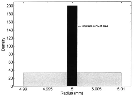
We build a model which depends on its radius. The manufacturer guarantees that every bearing has radius r between 4.99mm and 5.01 mm and that 40% of their bearings are between 4.999mm and 5.001 mm.

We need to represent the uncertainty in the radius of a particular bearing, for use in the model. In this physical example, the radius could be any distance and so a continuous Random Variable is appropriate. Because we lack additional information about the probability densities, we choose to describe the radius with Random Variable R (wR). The probability density function is:

A

fR (r 161 4.99 <r <4.999

1161

5.001

< r < 5.01

fR (r) is shown in Figure 2-1. The outcome space is OR = [4.99,5.01] and each value r within the inner bounds is 9 times as probable as the other values.

200- 180- 160-<- Contains 40% of area 140- ->, 120 -CD E 100 - 80-60- -40- - 20-0 4.99 4.995 _{5 5.005 5.01} Radius (mm)

Figure 2-1: The probability density function of the uncertain bearing radius in Example 1

Section A deals with more advanced concepts in probability theory and reconciles general prob-ability theory with the narrow definition that we use.

2.2.2 Statistics

Statistics as a field is concerned with interpreting data. In this work, we use statistics in two ways: estimating model parameters given a new dataset, and estimating properties of a hypothetical population represented by a probability distribution. The estimation techniques are discussed later in Section 6.2. Here we define some basic statistics of probability distributions.

Mean/ Expected Value

As with most statistics, the expected value of a Random Variable is computed using the prob-ability density function. For continuous Random Variables:

p

=

(x) fx (x) dx

This is simply the weighted average of all the values the Random Variable can take. The subscript in Ex [X (w)] indicates that the values of the argument X (w) will be weighted by the probability density function of X. This is more clear below:

Ex [g (X (w))]

=

g

Here, the Expected Value are the values of the argument, which is a function of the values x, are weighted by probability density function fx (x).

Mode

The mode is the value (or values) with highest probability density.

arg max fx (x)

Median

The median is the value which has half the probability mass below and half the mass above.

xmedian 0Z

J

fx (x)

dx

=

fx

(x) = 0.5

-o0 xmedian

Variance

The variance of a Random Variable X (w) measures the spread of the values x around the mean

Yt.

a.2

0.

₌

_-

_[X])2fx

_dx

£2x

Skewness

The skewness of a Random Variable is a measure of how the values are balanced around the mean p. For example, a small density of values far greater than p can be balanced by a large density of values slightly less than p. This would cause a positive skew. For some densities this is analogous to symmetry but a density can be asymmetric and unskewed.

-y = Ex

3

Descriptive Worth

Each statistic provides a different description of a Random Variable. No single statistic can completely characterize all Random Variables - some statistics are very informative for particular Random Variables but do not capture interesting behavior of other densities. For example, mean and variance completely define the Gaussian and continuous Uniform distributions, but can be con-fusing on bimodal distributions. Therefore it is important when describing uncertainty to consider which metrics are most appropriate and can give valuable descriptions of a wide range of Random Variables. This will come up again in Section 2.3.

Example 2: Visual Descriptions of Uncertainty Using Probability Theory

Figure 2-2 shows the standard Gaussian distribution and the standard lognormal (the log of this Random Variable is the standard Gaussian). The credible intervals are a Bayesian equivalent of confidence intervals. They show the mean (squares), median (diamonds), 68.2% credible interval (inner end points of lines), and 95.4% credible interval (outer end points). The x-credible interval is centered on the median, and covers 1% of the values above and below the median.

0.8 0.4- - * 0.6-0.3 e 0.4-- 0.2 -0.1- 0.2 -3 -2 -1 0 1 2 3 0 2 4 8 x x

(a) Gaussian (b) Lognormal

Figure 2-2: Example 2 - Random Variables representing uncertainty are shown as histograms, functions, and credible intervals.

2.2.3

The Gaussian Distribution

The Gaussian distribution is the most commonly used Random Variable for describing uncer-tainty. One reason is that natural populations often have attributes that are well approximated by the Gaussian distribution. In addition, it is a convenient modeling tool because it has very nice statistical properties. For example, summing Gaussian Random Variables results in another Gaus-sian Random Variable. Also, the entire distribution can be completely defined by two statistics: mean and variance.

To explain why the Gaussian distribution is not always appropriate, we describe the central limit theorem and contrast it with the phenomena associated with physical systems. An in depth discussion can be found in the Ph.D. Thesis of de Mann [17].

The Central Limit Theorem

Let Ym (wy) for m = 1... M be a series of Random Variables, all of which have the identical,

M

non-Gaussian distribution with mean y and finite variance a2_{. Then let}

SM (wy) E Ym (WY).

i=1

The central limit theorem states that as M -+ oo, the distribution of SM (wy) will approach a

nor-M

mal distribution So (wy) ~ N (p, o-). By rescaling, ZM (Wy) =1will approach

the standard Gaussian Z. ~ N (0, 1).

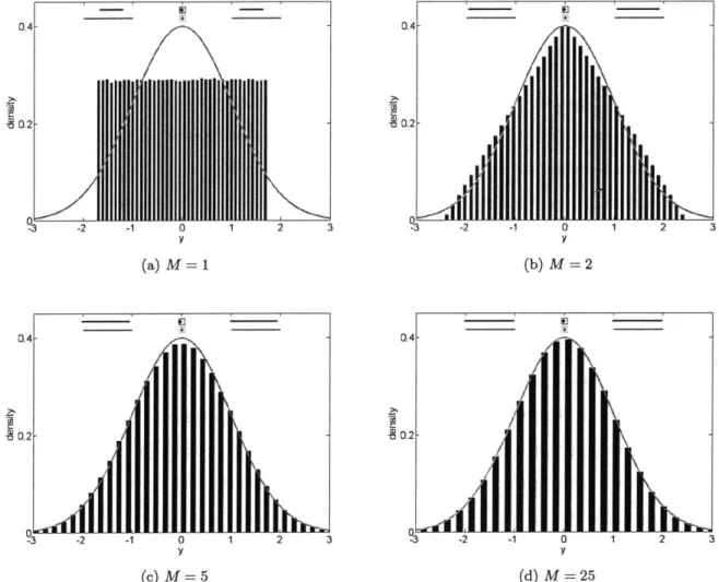
Example 3: The Central Limit Theorem

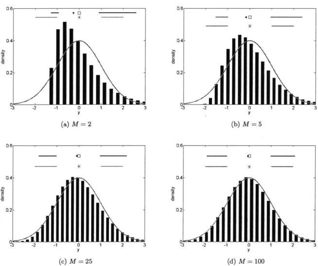
The Central Limit Theorem is illustrated by plotting the probability density function of SM (Wy) for increasing values of M for two distributions: the uniform distribution Ym (Wy) ~ U (0, 1) in Figure 2-3 and the exponential distribution Ym (wy) ~ Exp (1) in Figure 2-4.

The closer that the original distribution of Ym (wy) is to Gaussian, the smaller M needs to be

for ZM (Wy) to approach the normal distribution.

The Central Limit Theorem and Physical Systems

There are two problems with using the central limit theorem to justify modeling physical phe-nomena with Gaussian distributions. This assumes that all the underlying variations that cause the uncertainty are identically distributed and present in infinite number. The first assumption can be relaxed under certain conditions but the second is the larger concern. There may be a very large number of sources of uncertainty but only a handful will be significant. In that case, we are not looking at an infinite sum of Random Variables but a finite and rather small sum. This new

scenario is examined in Example 4.

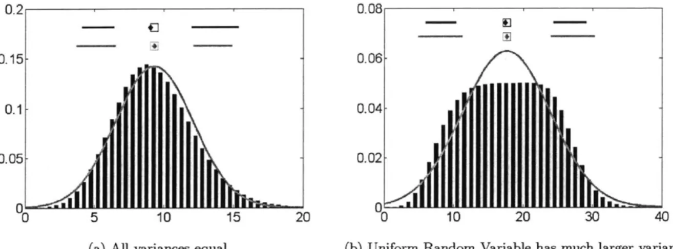
Example 4: When the Central Limit Theorem Does Not Apply

Here we look at the sum of eight different distributions (Gaussian, x2, lognormal, exponential, uniform, beta, Poisson, and gamma). This is a more realistic scenario that might be observed in practice in that there are only a small number of significant uncertainties. Figure 2-5a shows an example where many sources of uncertainty combine to produce a Gaussian uncertainty. This occurs when each of the Random Variables has (approximately) equal variance. Figure 2-5b shows

2 0. (a) M =1 (b) M=2 4- 2-y (c) M = 5 2 3

Figure 2-3: Example 3 - The scaled sum of M uniform Random interval) approaches the standard Gaussian (- & bottom credible

0

y

M=25

Variables (bars & top credible

interval) as M -+ oo

.D.

0.

.2 - -

.4-.2-j

Figure 2-4: Example 3 - The scaled sum of M exponential Random Variables (bars & top credible interval) approaches the standard Gaussian (- & bottom credible interval) as M -+ oo

an example where many different distributions are summed together, however, one of them has a larger variance than the rest. Note that these sums are not scaled, so the target is not the standard Gaussian. The Gaussian density function shown is fitted to the mean and variance of of the summation density.

0.2 0.08 0.15- 0.06-0.1- 0.04 0.05- 0.02 0 0 0 5 10 15 20 0 10 20 30 40

(a) All variances equal (b) Uniform Random Variable has much larger variance

Figure 2-5: Example 4 - The unscaled sum of eight Random Variables (bars & top credible interval) versus a Gaussian distribution (-) neither is a perfect Gaussian distribution

Intuitively, if one source of uncertainty is larger than the others, it will dominate the sum. This example shows that while the Gaussian distribution is a good approximation for some systems, it is not universal.

Functions of Gaussian Random Variables

In addition to the fact that not all sources of uncertainty can be represented with Gaussian Random Variables, a non-linear model will very rarely have Gaussian model prediction uncertainty. This is illustrated in Example 5 with the simplest possible model.

Example 5: Gaussian Parametric Uncertainties in a Linear Model

Our model is ax = b. Both a and b are uncertain parameters with Gaussian probability density functions, and we want to know the density of x.

This is modeled as X (wx) = . The results are shown in Figure 2-6 for several choices of

(WB)-(a) A (WA) ~ N (1,0.12) and B (oB) ~ N (4, 0.12)

lg0. W, '0

~0

(c) A (WA) - N (1,0.12) and B (WE) ~ N (0.4, 0.12)

(b) A (WA) ~ N (1,0.12 ) and B (WB) ~ N (1,0.12 ) 0.8- ] C Q4 (d) A ( 0 5 10 (d) A (WA) - N (1,o0.3 2 ) and B (WB) , N (1,12)

Figure 2-6: Exam le 5 - Probability density function of the ratio ables, X (wx) =

of two Gaussian Random

Vari-4

-Not only is the output non-Gaussian, the probability density function can vary widely depending on the parametric uncertainties. A Gaussian approximation of the output would be a very poor choice.

2.2.4 Rigorous Modeling of Uncertainty

Probability Theory allows for a rigorous description of uncertainty. However, in the past the Gaussian distribution has been used to describe almost all uncertainties. This greatly simplifies the analysis but as shown in the above examples, this is not always a valid assumption. Accurate analysis must begin with an accurate description of uncertainty, meaning that full probability density functions must be used. Variance is a useful statistic that can describe the spread of an uncertain parameter, but as was discussed in Section 2.2.2 it is not the only metric. Other statistics have been created that are better suited for describing the property we are most interested in: information.

2.3

Information Theory

Information theory was developed in the 1940's to answer questions of how fast and how reliable communication methods could be. Along the way, the theory also established metrics for the information content of a random event. While this rather abstract idea has its uses for data compression, it has had a wide ranging impact on practical devices like music players and cell phones. The problem of interest is how to compare two random events and measure them on some common basis. According to information theory, Random Variables can be ranked in terms of the information content they convey [52].

In the Bayesian approach to modeling, probability theory and Random Variables represent the uncertainty of a parameter and the knowledge we have about that parameter. Information theory statistics are then used to describe the information content of these Random Variable. For decision theory and design of experiments, these statistics are necessary to quantitatively measure the usefulness of each experiment. This is the basis of determining the best experiments during the design process.

By far the most common statistic for describing uncertainty is variance. When dealing with

however as stated in Section 2.2 not all uncertainties should be represented with Gaussian Random Variables. This section discusses the properties of the variance statistic and its limitations. Then the ideas of Shannon Information and the entropy statistic are introduced. Appendix B has more details about both as well as some supporting material.

2.3.1 The Variance Statistic

The variance of any Random Variable was given by Equation 2.1. Figure 2-7 shows two sets of probability density functions to illustrate this statistic.

0.75-

0.75-~0.5

~0.5

0.25 - --- -- - - -- 0.25

0 -3 -2 -1 0 1 2 3 OL-3 -2 -1 0 1 2 3

(a) Same variance (b) Same information content

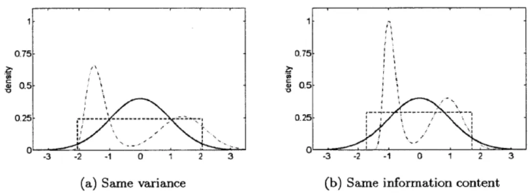
Figure 2-7: Two sets of probability density functions illustrating the two uncertainty statistics - all have mean 0

Variance is related to the spread of values around the mean. The three probability density functions in Figure 2-7a have variance of 1. The Gaussian Random Variables have most of their mass concentrated around the mean, but the tails of the distributions greatly increase the variance. The uniform Random Variable has no tails but this is balanced by having more density at an intermediate distance from the mean. The third is a mixture (combination) of a lognormal and Gaussian distributions. It has less density at the mean and has two modes, which greatly increases the variance.

If these densities in Figure 2-7a were representing an uncertain parameter, what would they

tell us? The Gaussian and mixture densities indicate that the true value is much more likely to be near the the modes, respectively 0 and -1 and 0.9. The uniform density does not indicates a most likely true value but does limit the possibilities to between ±1.7. Intuitively, these three densities convey a different amount of information about the parameter. Although variance does describe

one facet of how much information a variable contains, it does not convey this interpretation of information. Figure 2-7b shows the same distributions, but with new parameters. The mixture and Uniform Random Variables now have higher variances; they are set to have equal information

content, averaged over the whole density. This statistic is explained below.

2.3.2

Shannon and Differential Entropy

Shannon Entropy is an information metric defined for discrete random variables. Higher entropy corresponds to lower information content. The analogous statistic for continuous random variables is the differential entropy. The formula of differential entropy of the random variable 0 is:

h (X (w))

-

J

fx (x)log fx (x) dx

For uncertain parameters, high entropy indicates that a lot of data is required to learn the true value. Lower entropy indicates that a lot is already known about the uncertain parameter and less data would be required to learn the true value.

2.3.3

Kullback-Leibler Divergence

Like probability density functions, the differential entropy is a relative quantity because its absolute value is not meaningful. It must be stated along with a reference point. One way to do this is to simple compare the differential entropy of two Random Variables. This gives a measure of information gain. Another statistic is the Kullback-Leibler Divergence:

DKL (X (oJ) Y()) = -fx () log

0

The Kullback-Leibler divergence DKL is conceptually similar to a 'distance' between two probability density functions that share a underlying probability space, in this case denoted by the shared value (. This occurs, for example, when the two Random Variables being compared represent two characterizations of the same uncertain parameter. The Kullback-Leibler divergence will be used as an information metric for design of experiments. Instead of information gain from one density to another, this is a measure of how different the densities are. It can be interpreted as the