Publisher’s version / Version de l'éditeur:
Vous avez des questions? Nous pouvons vous aider. Pour communiquer directement avec un auteur, consultez la
première page de la revue dans laquelle son article a été publié afin de trouver ses coordonnées. Si vous n’arrivez
Questions? Contact the NRC Publications Archive team at
[email protected]. If you wish to email the authors directly, please see the first page of the publication for their contact information.
https://publications-cnrc.canada.ca/fra/droits
L’accès à ce site Web et l’utilisation de son contenu sont assujettis aux conditions présentées dans le site LISEZ CES CONDITIONS ATTENTIVEMENT AVANT D’UTILISER CE SITE WEB.
Student Report (National Research Council of Canada. Institute for Ocean Technology); no. SR-2007-12, 2007
READ THESE TERMS AND CONDITIONS CAREFULLY BEFORE USING THIS WEBSITE. https://nrc-publications.canada.ca/eng/copyright
NRC Publications Archive Record / Notice des Archives des publications du CNRC : https://nrc-publications.canada.ca/eng/view/object/?id=a6b1ed01-7f60-4afc-91f2-7f3ddfa015b9 https://publications-cnrc.canada.ca/fra/voir/objet/?id=a6b1ed01-7f60-4afc-91f2-7f3ddfa015b9
NRC Publications Archive
Archives des publications du CNRC
For the publisher’s version, please access the DOI link below./ Pour consulter la version de l’éditeur, utilisez le lien DOI ci-dessous.
https://doi.org/10.4224/8895002
Access and use of this website and the material on it are subject to the Terms and Conditions set forth at
Survey, analysis and validation of the IOT computer network
DOCUMENTATION PAGE
REPORT NUMBER
SR-2007-12
NRC REPORT NUMBER DATE
August 17 2007
REPORT SECURITY CLASSIFICATION
Unclassified
DISTRIBUTION
Unlimited
TITLE
Survey, Analysis and Validation of the IOT Computer Network
AUTHOR(S)
Robert Lockyer
CORPORATE AUTHOR(S)/PERFORMING AGENCY(S)
National Research Council –Institute for Ocean Technology
PUBLICATION
SPONSORING AGENCY(S)
National Research Council – Institute for Ocean Technology
IMD PROJECT NUMBER
421020
NRC FILE NUMBER KEY WORDS
PC Network, Ping, Survey
PAGES 19 FIGS. 17 TABLES 0 SUMMARY
This report gives a brief introduction to network protocols, an overview of the IOT computer network, detailed instructions on how to perform a network survey and the results of the author’s tests on the IOT network. The most peculear of these results are the periodic spikes in latency exibited by a switch located in telecommunications closet six. This behaviour was not repeatable in any other switches. Speculation points to virtual local area networks (VLANs) or hardware issues as possible causes. It currently does not seem to be affecting network performance in any noticable way. It is recommended that this switch should be checked periodically to discover if the anomaly develops any further.
ADDRESS National Research Council
Institute for Ocean Technology Arctic Avenue, P. O. Box 12093 St. John's, NL A1B 3T5
National Research Council Conseil national de recherches
Canada Canada
Institute for Ocean Institut des technologies
Technology océaniques
SURVEY, ANALYSIS AND VALIDATION OF THE IOT COMPUTER
NETWORK
SR-2007-12
Robert Lockyer
TABLE OF CONTENTS
1.0 INTRODUCTION ...1
2.0 NETWORK PROTOCOLS ...1
2.1 The Open Systems Interconnection Model...1
3.0 IOT NETWORK STRUCTURE...2
3.1 External Network Connections ...3
3.2 The Firewall...4
3.3 The Core Routing Switch...4
3.4 Network Closet Switches...4
3.5 Personal Computers...5 3.6 Servers ...5 3.7 Beowulf Clusters ...5 4.0 SOFTWARE...5 4.1 Ping ...6 4.2 Fping ...6 4.3 Cut...6 4.4 Awk ...7 4.5 Excel...7
5.0 RUNNING THE TESTS ...7
5.1 Laptop Setup ...7
5.2 Using Fping to Collect Network Data...8
5.3 Filtering Data Using Cut ...9
5.4 Awk ...12
5.5 Importing the Data Into Excel ...12
5.6 Graphing the Data ...13
6.0 RESULTS ...13 6.1 TC6 ...14 6.2 Data ports...16 7.0 CONCLUSION ...17 7.1 Recommendations ...17 BIBLIOGRAPHY ...19 LIST OF FIGURES Figure 1. ISO/OSI Model...1
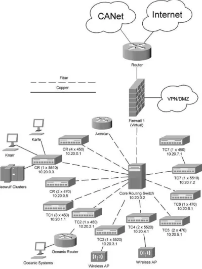
Figure 2. IOT Network Configuration (simplified) ...3
Figure 3. By default Fping only indicates if the device is alive or unreachable...8
Figure 4. fping command (pings each address from the file ip_list 5 times)...9
Figure 5. fping command (saves results to a file)...9
Figure 6. The useful data can easily be cut out of this file...10
Figure 7. First cut ( cut –d= -f3 file ) ...10
Figure 13. Table of average Ping Delays ...14
Figure 14. 200 consecutive pings ran directly on TC6...15
Figure 15. 200 consecutive pings ran directly on TC5...15
Figure 16. Ports tested by pinging 1Gbps network hardware ...16
Figure 17. Ports tested by pinging 100Mbps network hardware ...17
APPENDICIES
Appendix A: Diagrams Appendix B: Graphs Appendix C: Data
SURVEY, ANALYSIS AND VALIDATION OF THE IOT COMPUTER NETWORK 1.0 INTRODUCTION
This report aims to give the reader a comprehensive understanding of how to survey a computer network and how to subsequently analyze the data that is collected. Specifically, it discusses the results of tests ran by the author on the IOT computer network. Furthermore, this report discusses in depth the layout of the IOT network in order to give the reader a better understanding of how the systems being tested are organized. Someone with some understanding of computer networking should be able to utilize these methods on their own network, thereby gaining important information they may have otherwise overlooked.
2.0 NETWORK PROTOCOLS
A network protocol is simply a programmed procedure that two or more computers use to communicate with each other. Most modern computer networks like IOT’s are based on the Transmission Control Protocol and Internet Protocol. This combination is usually abbreviated as TCP/IP.
The International Standards Organization (ISO) developed the Open Systems Interconnection Model (OSI) as the standard for computer networking protocols. It contains seven separate layers each of which serve a distinct role. Although the OSI model has never caught on in terms of practical implementation it is still used as a tool in the analysis and discussion of computer networks.
The two columns of boxes represent two separate machines each running their own network stack. The vertical arrows indicate the interfaces between each layer. While the horizontal arrows indicate the transfer of data across the network.
Each layer does not directly communicate with its pair on the opposite host, this only occurs virtually (with the exception of the physical layer). The actual path of information is from the application layer down each layer one by one to the physical layer and then across the physical connection and back up the opposite stack. Although the actual transmission of data resembles a “U” shape, the various layers can be programmed as if they really transmitted directly across to their twin in the other stack.
The physical layer consists of the network hardware and drivers (software which directly controls hardware). Things like network cards and Ethernet cables make up the physical layer. The Data Link layer consists mostly of mechanisms for error detection and correction. The Network layer operates the addressing and routing procedures this is where devices such as IOT’s core routing switch operate. Other less elaborate switches are likely to reside on the physical layer or Data link. The transport layer splits the message from the session layer up into smaller pieces that the network layer can send as packets. The session layer establishes synchronization and sessions to allow for activity such as file transfers. The presentation layer converts data from its native format into a network useable form and back again. Finally, The application layer consists of the programs that you use on your computer, such as your email client and web browser that allow you to interface with your computer and let you talk to another piece of software on another computer.
It is important to note that the Physical Layer does not need to be copper wire. It can be a wireless network, or fibre optics, or any other means of information transmission. The rest of the stack will remain functioning as long as the adjacent layers receive the same information at their interfaces. In fact, this is true for any layer. It is extremely common at the Application Layer. The user is constantly changing applications all of which must interface with the Presentation layer in the same way. The modular construction of the OSI model allows for very flexible computer networks.
3.0 IOT NETWORK STRUCTURE
The IOT network consists of over 300 computers and various other devices spread throughout the building. They are all connected together using either copper or fibre optic cable. Also, a wireless network is now in operation in the Tow-Tank-OEB area of the Institute. As with most modern networks one can visualize the IOT network as an
upside down tree with the roots being the connections to the outside networks and the leafs being individual computers which branch off switches, and other network devices.
Figure 2. IOT Network Configuration (simplified)
3.1 External Network Connections
At the roots of the IOT network “tree” are the Internet and Canada’s Advanced Network (CANet). CANet is a Canada wide network of research institutions such as NRC and various universities. It operates at much higher speeds than the commercial Internet allowing efficient communication between Canada’s various research institutions.
Connected to the two outside networks is a router. A router is a device that directs traffic between two or more otherwise individual networks. It manages IOTs connections with CANet and the Internet. It also functions as a packet filter by blocking access to specified ports. It is connected directly to the firewall.
3.2 The Firewall
There are in fact two firewalls, but only one of them is actively filtering network traffic at any given time. The other simply provides a layer of redundancy in case the primary fails. These firewalls connect to the VPN, which lets employees connect remotely from an outside network and then appear as if they are on the inside, giving them the ability to map drives and use their computers remotely. It also connects to the De-Militarized Zone (DMZ), a security zone logically outside of the firewall. Devices that need to be less protected reside in this zone. They need to be visable on the Internet, unlike the rest of the network. Web and email servers are common in DMZs because they need to be viewable by the public. The firewall also connects to the core routing switch the core routing switch (the Nortel Passport).
3.3 The Core Routing Switch
The core routing switch in the computer room interfaces with other networking equipment using fibre data cable. Fibre is used because copper is more prone to attenuation. Attenuation is the drop in signal quality as the length of the wire increases. A signal can travel much further through fiber without repeaters. This allows the distribution of network connections to distant parts of the building without using repeaters. Also the maximum bandwidth of fibre is much higher than copper. This makes fibre exellent for use in the backbone of a network where much higher bandwidths are required to prevent bottlenecks. The core routing switch connects to seven separate network closets across the building. Inside each network closet there is at least one switch. In some network closets several switches are linked together in order to provide more ports to connect more computers. The core routing switch also connects to a series of switches in the computer room, which provide connections for computers in the nearby area.
3.4 Network Closet Switches (Edge Devices)
The switches connect many computers in their nearby vicinity together and then connect across longer distances to the core routing switch and through that to each other and the Internet. In order to provide an extra level of control over the network these switches can deploy Virtual Local Area Networks (VLANs). VLAN’s allow the administrator to logically separate users normally on the same network into smaller independent LANs. At IOT VLANs are used to place various companys in the building on their own LANs separate from IOT and eachother. This provides additional security without the need for extra hardware, which could otherwise make the same configuration much more expensive and prone to failure.
3.5 Personal Computers
All of the personal computers which employees use connect to the seven network closet switches and the switches in the computer room. Each individual computer at IOT is named according to the following standard. It starts with “PC” and then a number follows usually of the form 00xxxx where x is any digit. The IP address then directly follows in the form 10.1.x.xxx. For example if a computer were named PC002133 its IP address would be 10.1.2.133. These IP addresses are private meaning that they are not visible on the Internet. They are controled internally. Public addresses must be licenced.
3.6 Servers
Attached to a main switch in the computer room are Knarr and Karfe and several other PC network server computers. Knarr and Karfe are Windows 2003 virtual server clusters that are hosted on two physical computers named Skide and Snekke. Windows server 2003 provides redundancy by running both systems as virtualizations so that if one server fails the other can operate the network by acting as both servers. This is a theme that is very recurrent in enterprise class networking architecture. Most companies cannot tolerate extensive downtime while a failed server is repaired or replaced. The objective of this setup is to avoid that downtime altogether. The hard drives used by these servers are arranged in a RAID (Redundant Array of Inexpensive Disks), which also takes this approach. A number of hard drives can fail without any loss of data. They can then be easily swapped out for new replacements.
3.7 Beowulf Clusters
The Beowulf clusters are large rack mounts filled with dual CPU (Central Processing Unit) computers, which are networked together so that they can share processing. This practice is often referred to as parallel computing. It is usually a lot cheaper to buy many inexpensive computers and link them together than it is to buy one large super computer with the equivalent processing power. The researchers use these Beowulf clusters to do CPU intensive numerical simulations of various structures and systems.
4.0 SOFTWARE
There were only a few pieces of software that were used in these tests, most of which is free or has open source equivalents. Ping comes with almost every operating system, so you should have no trouble finding it. Fping is common to most Linux distributions and so can easily be acquired for free along with the OS. Cut and Awk are even more common among Linux distributions. Excel is the only software used here that you may have to purchase, however it has an open source equivalent in the Open Office software suite that will probably work just as well.
4.1 Ping
The ping program was named after the sound that sonar systems make. That’s appropriate because it works in much the same way. Ping sends out a packet to another network device and then waits for a reply. It then calculates the length of time it took the packet to travel between the two machines. If the second machine doesn’t respond Ping will stop waiting after a several seconds and count that packet as dropped. Most implementations of ping will do this multiple times in order to establish a reliable average. This also allows you to detect if there is any kind of change in the connection over time. The Windows version of ping does this four times unless told otherwise, while the Linux version continues sending pings until ordered to stop. The biggest problem with the Windows over the Linux implementation is that it records anything less than a millisecond as 0ms where as the Linux version outputs up to three decimal places. This is usually not a problem if you’re working with Internet speeds. However, when you look at higher bandwidth networks most of your results will come out to 0 seconds. While this tells you that your connection is operating above a certain performance threshold, it really obscures a lot of other information that could be useful. However, there is another problem that the native ping program faces on either operating system. It is inefficient and therefore slow when you want to ping multiple machines. The modified version Fping offers a remedy to this situation and provides a few other benefits.
4.2 Fping
Fping works like ping for the most part with a few important exceptions. The most useful of these is that it can ping multiple computers at the same time. This is because it doesn’t wait to complete a series of pings on one device before it starts on the others. It effectively pings in parallel. This allows you to ping many machines in the time it would normally take to ping one. Another useful feature is that you can ping a list of IP addresses saved to a file. This saves you even more time again because you only need to write out the addresses once. The finial advantage of Fping is that its output is designed to be easy to parse. What this means is that it is a lot easier extract the numbers you need from the results than in ordinary Ping. The results of ping are in a big paragraph while Fping organizes its results into an easily readable series of lines with consistent format. This is because Fping is designed for implementation in scripts. This is useful because scripts will make filtering for the data you need a lot simpler.
4.3 Cut
Cut is another common Linux command. It allows you to parse a text file in order to retrieve the information you are interested in. You do this by specifying delimiters. Delimiters can be any symbol, but you want to pick something that shows up consistently throughout the file. Whatever you choose as your delimiter divides the text into columns wherever that symbol is found. You can then choose which columns to delete and which to keep by referencing their number. This is an extremely powerful tool, which will save you a lot of time sorting through data.
4.4 Awk
Awk’s creators define it as: a “pattern scanning and processing language”. You’ll need an interpreter like Mawk or Gawk in order to use it. The utility of it for these tests is rather simple, so it is not important to understand it in depth. It is only used to convert text files from Unix format into Windows format. To do this you need to use a command from Awk to find and replace Linux newline characters with their windows equivalents. An Awk interpreter should be standard with most Linux distributions. There are many other uses of awk that are not even mentioned here because it is only used briefly.
4.5 Excel
It is assumed that the reader has some experience with Excel because it is such a common office program. It has also been suggested that Open Office’s Calc program can be used in place of Excel the details of this haven’t been provided. It should be straight forward to convert the steps mentioned here to their equivalents in Calc. Excel is really just a simple way to create graphs. Therefore, if you have a better way to do that feel free to substitute your own method or program once you have your data collected.
5.0 RUNNING THE TESTS
The tests consisted of setting up a laptop to run Fping and using a list to ping all of the separate network closet switches along with the main computer room’s switches and the passport. This was performed on a total of 44 different data ports throughout the building in order to get a good sample of the network. The important data was then extracted using Cut and the files were converted to Windows format using the sub command from the awk language. After that they were imported into excel and graphs were set up from the data. From these graphs any anomalies became apparent.
5.1 Laptop Setup
To start with you will need a copy of a Linux distribution that includes Fping. If you know how to download and install Fping yourself you can easily do it that way too but most current distributions seem to come with it, so it is assumed you have it on yours. The author used Knoppix Linux version 4.0 when doing the actual tests. However, to make screenshots he used Ubuntu Linux version 5.10. Both contain most of the programs you need. It is recommend that you install the operating system fully. If your using a live CD, every time that you restart you’ll lose your data unless you have it stored on some sort of external media like a flash drive. Also, it seems as if the first few pings are slower when using the live CD. This isn’t overly surprising because the live CD runs off the ram slowing down the operating system significantly. Fully installing Linux is better than a
The laptop you use isn’t terribly important to the tests. As long as it is not exceptionally old it should have an Ethernet jack that you can connect the cable to for testing. Furthermore, you need a system that has supported hardware under the Linux distribution that you’re planning to use.
5.2 Using Fping to Collect Network Data
There are several ways to automate Fping to make collecting the data you need in a timely manner easy. These steps require some initial work but quickly pay off in the speed with which you will be able to collect data once you have the procedures set up and operating. The Fping program has various switches, which allow you to modify its behaviour from the default. By default it will only tell you if a network device is alive or unreachable! Of course you would like to know a lot more information than that.
Figure 3. By default Fping only indicates if the device is alive or unreachable The first thing to be sure of is that you are getting accurate data from each computer. This requires performing more than one ping per device. This allows you to take the average of a few separate pings and reduce the effect of outliers. To do this in Fping you can use the “-c” option. After typing “-c” type a number that will determine how many times each target gets pinged. This will also provide you with information regarding how long each ping takes.
You also want to be able to ping more than one machine at a time. In order to do this you are going to have to use the “-f” option. This option allows you to choose a file to draw your list of IP addresses from. You have to create a file in your text editor that is simply a list of the IP addresses of the devices you wish to test in the order you wish to
test them in. This call of Fping is shown bellow in Figure 4. You can replace ip_list with the path of your file containing a list of target IP addresses.
fping –c 5 –f ip_list
Figure 4. fping command (pings each address from the file ip_list 5 times)
Finally, You are going to want to save the results to files so that you can access them later. To do this you simply have to redirect the standard error message. You can do this using two angel brackets proceeded by a “2” so it should look like “2>>”. The finial call to Fping is shown in Figure 5. You can replace “filename” with the path of the file you wish to save the output to. Keep in mind this will append extra data to the same file if you don’t change the name each time you use it.
fping –c 5 –f ip_list 2>>filename
Figure 5. fping command (saves results to a file)
This command was run on each data port with a different filename for each one. They were labelled the same so that they could be referenced later.
5.3 Filtering Data Using Cut
Using the Linux command “cut” you can extract the data you need from the output that Fping produces. The cut command’s syntax is rather simple and easy to learn. All you have to do is specify a delimiter in the data and it will divide the content into columns where those symbols show up. From there you can pick which columns to keep.
Figure 6. The useful data can easily be cut out of this file
Figure 6 shows a file formatted the same way as the files that were created from the tests. If you are working with a file similar to Figure 6 then you probably just want the average ping. That’s the second last column of numbers. You want to end up with a file that contains only a single column of those averages.
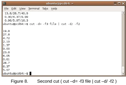
To use cut you first have to specify a delimiter, this tells the computer where to divide the file into columns. Then you can choose which to keep and which to discard. To specify a delimiter you use the “–d” switch. Place the symbol you wish to use as the delimiter directly after it. In this case, you could do it all in one instance of cut by using a forward slash symbol as the delimiter. However, it is a lot easier to see that there are 3 columns separated by “=” signs. [Figure 7]
If you choose the “equals” sign as your delimiter you will need the third column. To choose columns you have to type “-f#” where “#” is the number of the columns you wish to keep. The command and its results are shown in Figure 7.
Choose the forward slash as your next delimiter. This cuts the data into three more columns; you want the center column “average ping” from each so you specify the second column. But in order to allow this new command to work with the data resulting from the previous cut you need to pipe the results. To use a pipe in the Linux command line, simply type "|” between two commands. This is shown in greater detail below. [Figure 8]
Figure 8. Second cut ( cut –d= -f3 file | cut –d/ -f2 )
Finally you want to save this data to a file so you will be able to import it into Excel. In the shell, to redirect the output of a command into a file you use double angle brackets “>>”. The final cut command is shown bellow in Figure 9.
cut -d= -f3 filename | cut -d/ -f2 >> outputfile
Figure 9. The cut command outputting to a file
Your going to have a lot of files to work with and this could get tedious unless you script it into a “for” loop. If you have any experience with programming you know what a “for” loop is. If you haven’t it is simply a method of programming that allows you to repeat an action based on a condition. In Figure 10 below, the command can just as easily be written on a single line.
cut -d= -f3 $f | cut -d/ -f2 >> ../cutfiles/${f}; done
Figure 10. The cut command scripted into a “for” loop
In this case the condition is “for f in *” star is a wildcard for “any filename”. The result is that it will run this command on every file in a directory. For loops in the shell require “do” and “done” to specify where they start and stop. This is a different syntax than C++ where you use curled brackets for the same purpose. The “$f” symbol is a variable that was set in the “for” loop to be whatever the filename of the current file is. Using this command you can take a directory containing hundreds of files and parse all of them for the desired information in seconds.
5.4 Awk
If your using Excel on windows to read these files it is useful to have them converted to the windows text format. To do this you need to do a “find and replace” operation using awk. You can add this to your current “cut” command in order to do the two operations in one script. for f in *; do cut $f -d= -f3 | cut -d/ -f2 | awk 'sub("$", "\r")' >> ../cutfiles/${f}.txt ; done
Figure 11. The Awk command added to the cut script
The only difference is that the line “ awk ‘sub(“$”, “\r”)’ “ has been extended. This simply takes any “$” symbols in the text file and replaces them with the escape character “\r” which is the windows newline character. Now all of the data should be ready to import into excel.
5.5 Importing the Data Into Excel
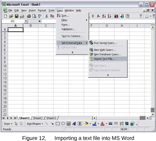
After the data has been filtered it will be easy to import it into excel. To do this on the file menu go to: Data >> Get External Data >> Import Text File [Figure 12]
Figure 12. Importing a text file into MS Word
Then locate the file you want to import, select it and click import. In the text import wizard click finish.
5.6 Graphing the Data
Now that you have your data set imported you should be able to arrange it into a suitable table and use the graph wizard. Select the data you want on your graphs and on the file menu go to: Insert >> Chart. From there you can choose a name for your graph, its x-axis and y-axis and set its visual appearances.
6.0 RESULTS
During my test there was one obvious discrepancy. TC6 showed a delay many times that of any other gigabit switch tested. The average delay across all gigabit devices excluding TC6 was about 1.48 ms. However, TC6 clocked in at an average of approximately 28.27 ms. Not only does this far exceed the gigabit devices, it is by far the longest average delay overall. The next highest is (CR 4) a 450 with an average ping delay of 20.44ms. That makes for a percent difference of 27.70%. The next highest percent difference between 100Mbps devices was 13.55%. This is a very significant
Average ping delay measured from multiple data ports 0 5 10 15 20 25 30 TC1 3(450) TC2 1(450) TC3 1(5520) TC4 2(5520) TC5 2(470) TC6 1(470) TC7 (1) 1(450) TC7 (2) 1(5510) Passport CR 4(450) CR 1(5510) CR 1(470) Device Name A v e ra g e r o u n d t ri p t im e f o r a 5 6 b y te p a c k e t
Figure 13. Table of average Ping Delays
All other switches performed as expected. However upon further testing it was realized that the switches didn’t react exactly the way that was predicted. Any device that was pinged behind the switch actually responded faster than the switch itself. It could be that the hardware interface for switch management is actually slower than the rest of the switch ports. This is easily conceivable, considering that it doesn’t take much bandwidth to modify the switches properties and that the other ports would be expected to perform at the rated speed. A manufacturer could probably cut costs by running a slower interface for switch management.
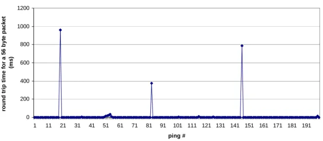
6.1 TC6
Upon further inspection of TC6 it was found that the reason for such a high average ping was caused by periodic delays. The switch performed as it should for the most part but every couple of minutes it would delay for extremely long durations. This became apparent in tests ran directly on the switch. [Figure 14]
Ping return trip time tc6 baystack 470 (measured from direct connection to tc6) 0 200 400 600 800 1000 1200 1 11 21 31 41 51 61 71 81 91 101 111 121 131 141 151 161 171 181 191 ping # ro u n d t ri p t im e f o r a 5 6 b y te p a c k e t (m s )
Figure 14. 200 consecutive pings ran directly on TC6
An identical test was also run on TC5, as a control [Figure 15]. This is the closest one could get to actually running it on the same hardware. It is not a perfect control because it’s actually two 470s linked together. It has been assumed for the time being that this is representative of normal behaviour because an identical piece of hardware was not available to compare TC6 with.
Ping return trip time for tc5 2 baystack 470s (measured from direct connection to tc5)
0 2 4 6 8 10 12 14 16 18 1 11 21 31 41 51 61 71 81 91 101 111 121 131 141 151 161 171 181 191 ping # ro u n d t ri p t im e f o r a 5 6 b y te p a c k e t (m s )
The two graphs are very similar in that they both form a flat straight line with two or three spikes. The only significant difference is the magnitude of the spikes. Applied to the same scale as TC6, TC5 would appear merely as a flat line.
It could be the result of using (Virtual Local Area Networks) VLANs on the switch. VLANs are a way of logically segmenting a network that is performed using the switches firmware. If this is a resource intensive process it could explain why TC6 is experiencing the issues it is. It may be that VLAN performance takes priority over the management firmware.
6.2 Data ports
For the analysis of the various ports TC6 was excluded. The random nature of its delays would skew the data that was being analysed. Upon examination of each data port for average latency and comparison to others, there are no significant discrepancies between the ports tested. The maximum delay for the Gigabit devices was 2.53 ms. The longest delay from the 100Mbps devices was 27.15ms.
Average Ping Latency of Various IOT Dataports from pinging Gbps network hardware
0 0.5 1 1.5 2 2.5 3 1-00 70 1-01 01 D 1-10 D 1-11 D 1-13 D 1-17 D 1-19 D 1-20 D 1-21 D 1-22 D 1-26 D 1-3 D 1-7 D 1-73 D 1-74 D 1-75 D 1-76 D 1-9 T1-8D1-13D1-41D1-45D1-42T1-2 1 D 1-40 D 1-38 D 1-46 D 1-47 D 1-50 D 1-48 D 1-49 1-01 04 1D-0 038 D-0 026 D-0 033 D-0 034 D-0 035 RD 1-13 1D-0 018 1D-0 020 1D-0 022 1D-0 025 1D-0 029 1D-0 030 Dataport L a te n c y ( m il is e c o n d s )
Average Ping Latency of Various IOT Dataports from 100Mbps network hardware
0 5 10 15 20 25 30 1-00 70 1-01 01 D 1-10 D 1-11 D 1-13 D 1-17 D 1-19 D 1-20 D 1-21 D 1-22 D 1-26 D 1-3 D 1-7 D 1-73 D 1-74 D 1-75 D 1-76 D 1-9 T1-8D1-13D1-41D1-45D1-42T1-2 1 D 1-40 D 1-38 D 1-46 D 1-47 D 1-50 D 1-48 D 1-49 1-01 04 1D-0 038 D-0 026 D-0 033 D-0 034 D-0 035 RD 1-13 1D-0 018 1D-0 020 1D-0 022 1D-0 025 1D-0 029 1D-0 030 Dataports L a te n c y ( m il is e c o n d s )
Figure 17. Ports tested by pinging 100Mbps network hardware
7.0 CONCLUSION
In conclusion, while TC6 seems to be experiencing some strange issues, the network is functioning normally despite this anomaly. It seems to be tied to a different component of TC6, one not directly involved in the networks communications. Possibly a part of the configuration management system. Another hypothesis is that the Virtual Local Area Networks setup on the switch are consuming system resources that could otherwise be used in responding to echo requests sent by the ping command in a timely manner. With the obvious exception of TC6 one can easily tell form looking at the graphs generated which switch is rated for Gigabit or 100Mbps. This is a good sign as it indicates that the network is operating as expected.
7.1 Recommendations
Due to TC6’s odd behaviour It is recommend that a test be ran on TC6 periodically, in case its minor issues balloon into bigger ones. It would be useful to have advance
Swapping TC6 with a similar switch would be the most useful, but disruptive test. One could see if the new switch behaved in the same manner. If so, one could conclude that this is simply the way that these switches react to this particular network environment. Another switch of a different model could also be used but such a test if a 470 does not become available.
BIBLIOGRAPHY
Cantin, Claude. Basic Introduction to UNIX/Linux. NRC, 2003.
Elms, Wayne 2007, Computer Systems Administrator, Institute for Ocean Technology. Interviewed by Robert Lockyer.
Sloan, D., Joseph, August 2001, Network Troubleshooting Tools. O’Reilly & Associates, inc., 1005 Gravenstein Highway North, Sebastopol, CA
Tanenbaum, S., Andrew, 1981, Computer Networks, Prentice-Hall, Inc., Englewood Cliffs, N. J.
Thorburn, Paul 2007, Computer Systems Administrator, Institute for Ocean Technology. Interviewed by Robert Lockyer.
Wadman, Ray 2007, Computer Systems Administrator, Institute for Ocean Technology. Interviewed by Robert Lockyer.
Walsh, Doug 2007, Computer Systems Administrator, Institute for Ocean Technology. Interviewed by Robert Lockyer.
Wong, Gilbert 2007, Computer Systems Administrator, Institute for Ocean Technology. Interviewed by Robert Lockyer.
APPENDIX A DIAGRAMS
APPENDIX B GRAPHS
1 -0 0 7 0 1 -0 1 0 1 D 1 -1 0 D 1 -1 1 D 1 -1 3 D 1 -1 7 D 1 -1 9 D 1 -2 0 D 1 -2 1 D 1 -2 2 D 1 -2 6 D 1 -3 D 1 -7 D 1 -7 3 D 1 -7 4 D 1 -7 5 D 1 -7 6 D 1 -9 T 1 -8 D 1 -1 3 D 1 -4 1 D 1 -4 5 D 1 -4 2 T 1 -2 1 D 1 -4 0 D 1 -3 8 D 1 -4 6 D 1 -4 7 D 1 -5 0 D 1 -4 8 D 1 -4 9 1 -0 1 0 4 1 D -0 0 3 8 D -0 0 2 6 D -0 0 3 3 D -0 0 3 4 D -0 0 3 5 R D 1 -1 3 1 D -0 0 1 8 1 D -0 0 2 0 1 D -0 0 2 2 1 D -0 0 2 5 1 D -0 0 2 9 1 D -0 0 3 0 TC1 3(450) TC2 1(450) TC3 1(5520) TC4 2(5520) TC5 2(470) TC6 1(470) TC7 (1) 1(450) TC7 (2) 1(5510) Core Routing Switch BCR 4(450) BCR 1(5510) BCR 1(470) 0 20 40 60 80 100 120 140 160 180 200 220 240 260 280 300 320 340 Data Port round trip time for a 56 byte packet (ms)
Network Device ping time of network devices measured from various data ports
APPENDIX C DATA
TC7 (2) 1(5510)Passport TC3 1(5520) TC4 2(5520) TC5 2(470) CR 1(5510) CR 1(470) TC6 1(470)Averages 1-0070 0.85 0.42 0.74 0.97 1 0.97 0.98 0.96 0.86125 1-0101 1.63 1.3 1.64 1.66 1.93 1.69 1.98 153 20.60375 D1-10 0.72 0.43 0.79 0.74 0.97 0.72 1.02 1.02 0.80125 D1-11 0.72 0.48 0.73 1.7 0.97 0.72 2.04 0.99 1.04375 D1-13 1.79 1.23 1.7 1.88 2.04 1.81 1.97 1.98 1.8 D1-17 0.79 0.45 0.76 0.75 1 0.72 0.99 1.01 0.80875 D1-19 1.8 1.25 0.81 0.75 0.97 1.73 2 1.98 1.41125 D1-20 0.71 0.38 0.75 0.75 4.32 0.73 1 0.97 1.20125 D1-21 0.72 0.41 0.73 0.74 0.97 0.72 1 0.99 0.785 D1-22 0.72 0.44 0.86 0.75 0.97 0.71 1 0.99 0.805 D1-26 1.66 1.26 1.71 1.68 2.03 1.67 1.94 2.21 1.77 D1-3 1.65 1.25 1.7 1.68 1.96 1.68 1.95 25.6 4.68375 D1-7 1.68 1.25 1.69 1.78 1.93 1.66 1.97 2.28 1.78 D1-73 0.72 0.41 0.74 0.74 0.95 0.71 1 1 0.78375 D1-74 0.71 0.43 0.74 0.75 0.95 0.79 1 277 35.29625 D1-75 1.68 1.31 1.71 1.68 3.72 1.65 1.94 1.95 1.955 D1-76 0.72 0.38 0.72 0.78 0.96 1.1 1 0.99 0.83125 D1-9 1.67 1.23 1.69 1.68 1.95 1.65 1.96 1.96 1.72375 T1-8 0.71 0.47 1.72 1.68 1.93 0.71 0.98 0.99 1.14875 D1-13 1.79 1.23 1.7 1.88 2.04 1.81 1.97 1.98 1.8 D1-41 1.67 1.39 2.41 1.7 1.96 1.67 1.99 1.97 1.845 D1-45 1.86 1.22 2.3 1.67 2.01 1.66 1.95 1.96 1.82875 D1-42 1.66 1.28 1.69 1.68 1.91 1.67 1.95 1.95 1.72375 T1-21 0.73 0.46 0.73 0.72 1.04 0.71 1.4 9.18 1.87125 D1-40 1.83 1.26 1.69 1.7 2.03 1.88 1.95 2.04 1.7975 D1-38 1.71 1.24 1.73 1.67 1.92 1.66 1.96 1.94 1.72875 D1-46 0.7 0.41 1.69 1.65 0.95 0.85 0.98 24.8 4.00375 D1-47 1.88 1.21 1.73 1.67 1.93 1.66 3.5 1.95 1.94125 D1-50 0.89 0.56 1.87 2.23 1.13 0.87 2.12 2.12 1.47375 D1-48 0.71 0.44 0.72 0.71 6.55 0.71 1.01 0.98 1.47875 D1-49 1.67 1.27 1.7 1.72 1.92 1.67 1.95 323 41.8625 1-0104 2.26 1.24 1.42 1.89 2.15 1.67 1.94 1.94 1.81375 1D-0038 1.65 1.27 2.36 1.68 1.95 1.25 2.41 316 41.07125 D-0026 1.28 0.39 0.71 0.83 0.98 1.14 0.98 1.08 0.92375 D-0033 2.08 1.2 2.52 1.67 1.95 1.27 2.19 21.2 4.26 D-0034 1.92 1.21 2.65 1.83 1.96 1.19 1.94 36.8 6.1875 D-0035 1.77 0.41 0.71 1.04 0.98 0.69 1 0.97 0.94625 RD1-13 1.83 1.34 2.27 1.68 2.04 2.54 2.32 2.25 2.03375 1D-0018 2.38 1.2 1.35 2.05 1.95 2.01 6.78 1.93 2.45625 1D-0020 2.3 1.2 2.42 1.38 1.94 1.37 1.92 1.93 1.8075 1D-0022 2.91 1.19 2.44 1.68 1.93 1.99 1.94 1.93 2.00125 1D-0025 2.15 1.22 1.66 1.64 1.94 1.58 1.93 1.94 1.7575 1D-0029 1.99 1.24 1.37 1.71 1.93 1.79 1.96 2.04 1.75375 1D-0030 2.27 1.3 2.58 1.68 2.17 1.59 1.89 2.06 1.9425 Averages 1.489545455 0.93545455 1.507954545 1.429545455 1.83590909 1.341818182 1.810227273 28.26841 4.827358
CR 4(450) TC7 1(450) TC1 3(450) TC2 1(450) Averages 1-0070 14.3 15.4 18.2 11.9 14.95 1-0101 26.3 17.8 18.2 20 20.575 D1-10 15.1 14.2 14.7 18.3 15.575 D1-11 31.1 17.5 17.8 15.7 20.525 D1-13 16.2 17.2 16.5 18.4 17.075 D1-17 15.8 14.6 15.9 16 15.575 D1-19 16.2 18.5 16.3 14.8 16.45 D1-20 15.4 13.3 23.2 19.3 17.8 D1-21 15.1 35 13.1 12.9 19.025 D1-22 15.5 13.5 13.6 13.2 13.95 D1-26 18.3 17.7 17.3 18.2 17.875 D1-3 29.1 15 17.8 16.6 19.625 D1-7 17.1 16.9 16.9 18.2 17.275 D1-73 34.8 20.6 14.3 14 20.925 D1-74 14.8 17.5 14.2 14.2 15.175 D1-75 17.7 17 19 16.8 17.625 D1-76 16.9 16.1 13.4 18.6 16.25 D1-9 20 17.6 17.2 16 17.7 T1-8 21.5 13.1 18.6 11.8 16.25 D1-13 16.2 17.2 16.5 18.4 17.075 D1-41 16.6 16.9 18.2 15.6 16.825 D1-45 24 16.7 18 18.8 19.375 D1-42 18.4 16.9 27.8 16.3 19.85 T1-21 15.9 15.5 13.5 21.1 16.5 D1-40 20.2 17.7 16.1 18.7 18.175 D1-38 16.9 18.2 18.8 20.5 18.6 D1-46 17.3 14 18.4 14.6 16.075 D1-47 18 17.6 18.9 20.9 18.85 D1-50 15.8 15 17.9 14.2 15.725 D1-48 15.9 13.4 18.3 13.6 15.3 D1-49 16.2 19.5 18.5 26.2 20.1 1-0104 17.7 17.7 29 17.6 20.5 1D-0038 50.7 16 17.8 16 25.125 D-0026 15.1 14.7 13.9 12.8 14.125 D-0033 52.6 16.9 16.4 16.5 25.6 D-0034 20.3 20.7 15.8 19.1 18.975 D-0035 14.2 16 16.5 14.7 15.35 RD1-13 20 23.3 19.7 35.5 24.625 1D-0018 21.3 18.3 15.8 16.3 17.925 1D-0020 17.7 18.6 26.2 17.7 20.05 1D-0022 28.1 17.5 17.1 18.9 20.4 1D-0025 23.6 35.4 20.5 16.4 23.975 1D-0029 18.8 16.7 19.3 16.3 17.775 1D-0030 16.8 18.5 36.8 36.5 27.15 Averages 20.4431818 17.66818182 18.225 17.6840909 18.50511364