Publisher’s version / Version de l'éditeur:
Vous avez des questions? Nous pouvons vous aider. Pour communiquer directement avec un auteur, consultez la première page de la revue dans laquelle son article a été publié afin de trouver ses coordonnées. Si vous n’arrivez pas à les repérer, communiquez avec nous à [email protected].
Questions? Contact the NRC Publications Archive team at
[email protected]. If you wish to email the authors directly, please see the first page of the publication for their contact information.
https://publications-cnrc.canada.ca/fra/droits
L’accès à ce site Web et l’utilisation de son contenu sont assujettis aux conditions présentées dans le site LISEZ CES CONDITIONS ATTENTIVEMENT AVANT D’UTILISER CE SITE WEB.
19th International Symposium on Ice [Proceedings], 2008
READ THESE TERMS AND CONDITIONS CAREFULLY BEFORE USING THIS WEBSITE.
https://nrc-publications.canada.ca/eng/copyright
NRC Publications Archive Record / Notice des Archives des publications du CNRC :
https://nrc-publications.canada.ca/eng/view/object/?id=e4a2195b-e8c7-456c-8c5f-246b8060ce38 https://publications-cnrc.canada.ca/fra/voir/objet/?id=e4a2195b-e8c7-456c-8c5f-246b8060ce38
NRC Publications Archive
Archives des publications du CNRC
This publication could be one of several versions: author’s original, accepted manuscript or the publisher’s version. / La version de cette publication peut être l’une des suivantes : la version prépublication de l’auteur, la version acceptée du manuscrit ou la version de l’éditeur.
Access and use of this website and the material on it are subject to the Terms and Conditions set forth at
Numerical implementation and benchmark of ice-hull interaction model
for ship manoeuvring simulations
19
thIAHR International Symposium on Ice
“Using New Technology to Understand Water-Ice Interaction” Vancouver, British Columbia, Canada, July 6 to 11, 2008
Numerical Implementation and Benchmark of Ice-Hull Interaction Model for
Ship Manoeuvring Simulations
Jiancheng Liu
P.O. Box 19, Faculty of Engineering and Applied Science,
Memorial University of Newfoundland, St. John’s, NL, Canada, A1B 3X5. E-mail: [email protected]
Michael Lau
Institute for Ocean Technology, National Research Council of Canada, St. John’s, NL, Canada, A1B 3T5.
E-mail: [email protected]
F. Mary Williams
Institute for Ocean Technology, National Research Council of Canada, St. John’s, NL, Canada, A1B 3T5.
E-mail: [email protected]
Abstract
The first question about the performance of a ship operating in ice is usually about the speed-power relationship moving ahead in the specified ice conditions. With advanced physical model test technology and the increasing scope and reliability of full-scale data on reference ships, this question may be answered with considerable confidence at the design stage. Attention has turned in recent years to assessment of the performance of ships undertaking turns and more complex maneuvers in ice. Ability to predict turning performance is important in ship navigation, and it is essential as the basis for numerical models in marine simulators used for operator training and operations planning.
This paper reports on the development of a new physically based ice-hull interaction (IHI) model, developed at the NRC Institute for Ocean Technology. This model will serve as the key ice component for ship real-time simulators in ice. The model calculates forces generated by increments in an arbitrary prescribed ship motion. The model incorporates multi-failure ice modes and hydrodynamic effects, and tracks the development of the broken channel. The theoretical basis for the model has been described in a previous paper. This paper presents the model’s numerical implementation and benchmarking based on ship model tests in ice.
Two series of physical model experiments carried out at NRC-IOT provided the benchmarking data. The reference ships are the Terry Fox icebreaker and CCGS R-class icebreaker. The model tests included resistance measurements, constant radius turns and sinusoidal manoeuvers using a captive model mounted on a Planar Motion Mechanism (PMM). The operating conditions included open water, level ice and pre-sawn ice. Ship motions and ice loads during the manoeuvers were measured in tests.
The PMM physical model experiments were realistically simulated using IHI model software. The calculated ice forces on the hull, the ice contact during the manoeuver and the width and shape of the channel formed were compared with physical measurements. The extensive experimental data sets enable verification of details of the mathematical model, as well as providing insight into the ship-ice interaction processes.
1. Introduction
Precise manoeuvering of a ship in ice is necessary in confined passageways and in the presence of navigation hazards. Navigation simulators, training simulators and autopilot systems are valuable tools to achieve precise control of a ship in a particular set of ice conditions. A new ice-hull interaction (IHI) model for the real-time simulations of ship manoeuvering in level ice was developed in NRC/IOT. The model will be integrated into the CMS training simulator as an ice force module in the original numerical framework. The model adopted an analytical approach with numerical implementation and was built on a detailed mechanical analysis of the hull-ice interaction in level ice. It considers the distributions of the breaking force, buoyancy force and clearing force using the corresponding theories. The adoption of the analytical approach yielded a short calculation time, which made the model suitable for real-time simulations. Since the forces were calculated at each new increment of any prescribed motion, the resulting simulation had the capacity to respond to arbitrary control inputs and hence arbitrary manoeuvers in ice. The conception and the corresponding theories of the model were introduced in Lau et al (2004). This paper focuses on its numerical implementation and benchmarking based on the ship model test data obtained at IOT.
A stand-alone numerical software using MatLab language was developed, which provided an independent numerical platform for developing and benchmarking the ice-hull interaction model. The model was benchmarked against measurements from two PMM ship model test series carried out at IOT, Terry Fox model tests (Deradjji and van Thiel, 2004; Lau, 2006) and R-Class model tests (Hoffmann, 1998). The comparison and analysis of physical tests and simulation results also provided insight into the ship-ice interaction processes and clues for further refinement of the model.
2. Brief description of model theories
The model estimates the ice forces needed for simulating the ship steady manoeuvering in ice in time-domain. It neglects the high frequency ice force fluctuation and integrates ice force over a large time interval consisted of at least a few ice broken cycles to arise at an average local ice resistance.
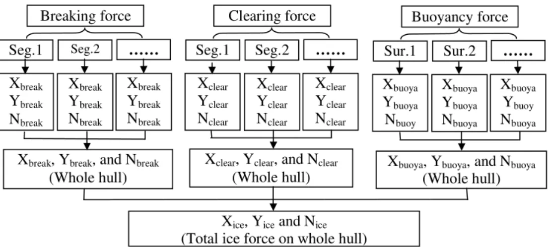
The total ice forces on the hull are calculated by the vectorially sum of the contributions from three independent force components, breaking force, buoyancy force and clearing force, which respectively represent the corresponding physical phenomena during the ship breaking ice process. clear buoy break ice X X X X = + + (1) clear buoy break ice Y Y Y Y = + + (2) clear buoy break ice N N N N = + + (3) Where X ,
Y
and N are the surge force, sway force and yaw moment respectively, and the subscripts “ice, break, buoy, and clear” refer to the total ice force, the ice breaking contribution, the ice buoyancy contribution and the ice clearing contribution respectively. The ice breaking forces components are mainly dependent on ice thickness, ice flexural strength, ice crushing strength, ice shear strength, ice elastic modulus, hull frame angles at waterline and ship velocity. The ice clearing force components are mainly dependent on ice thickness, hull wet surface and ship velocity. The buoyancy force component is mainly dependent on the ice-water density difference, hull wet surface and ice thickness.The whole hull was divided into many segments and the ice forces on each segment were calculated based on the ice-hull contact area and ship motions. The global ice forces on the whole hull were obtained through vectorially adding these forces and moments. Figure 1 shows a sketch of global force and yaw moment calculation in IHI model.
2.1 Breaking force calculation
When the ship turns, more parts of the hull may contact the unbroken level ice. In the model, the ice-hull contact area was calculated based on the ice edge and ship motion and the channel was tracked in time through a simple house-keeping method. A multi-failure model considering the bending, crushing and shear failures was used to check the ice failure at the waterline of the hull from stem to stern and the failure mode that required the minimum failure force was selected. A cusp ice crack pattern consistent with a 3-D plate theory governed the flexural failure and the channel formation. The average size of the broken ice pieces depends on ship speed, ice thickness and its mechanical properties with reference to Varsta (1983), Enkvist (1972) and Lau et al (1999).
2.2 Clearing force calculation
The IHI model calculates the clearing force component by considering the force imposed by the motion of an ensemble of ice pieces rotating and sliding along the submerged surface of the hull. The clearing force component includes viscous drag and inherent buoyancy for the rotating ice floes, forces caused by wave pressure and ventilation of the rotating ice floes, and inertial forces due to ice acceleration. The IHI model adopts an energy method to calculate the force imposed by the motion of the ice mass during the ice floe turning process. The force due to ventilation, the static pressure and bow wave on the ice piece turning at water surface, is estimated according to Enkvist (1972) and Kotras et al. (1983).
2.3 Buoyancy Force Calculation
The buoyancy component represents the lifting force by the submerged ice pieces due to the density difference between the ice and water. A simplified flat-plate model representing the underwater surface of the ship hull was used for buoyancy force calculation as shown in Figure 3. The model estimates the ice volume on each wetted surface of the flat-plate model in time domain.
3. Numerical Implementation of the Model
The developed ice-hull integration model software simulates the ice forces on the hull due to user-specified ship motions. The software allows direct inputs of ship geometry, prescribed ship motions, ice mechanical properties, and the initial ice edge geometry, and compute ice loads on the hull, ice-hull contact area, and channel configuration. The IHI model software is designed as a Visual Calculation Program (VCP). During the calculation process, the users can instantaneously watch the simulation process and check the simulation results, such as ship’s motion, ice channel and calculated surge force, sway force and yaw moment on the hull imposed by the ice. It is important for the users to visualize the physical process of the ice-hull interaction and for the developer to refine the model. The software has flexibility and refinement spaces for future development of the IHI model. It also has a friendly data exchange connection, which makes it easy to be implemented into other numerical frameworks as an interior module. The whole IHI code consists of three layers, Parameters Input Layer (PIL), Core Calculation Layer (CCL) and Results Output Layer (ROL). Figure 2 shows the software structure for the IHI model and the associated main m-files.
Additional details of the model theories and numerical implementation can be found in Liu et al. (2006, 2007a, 2007b).
4. Benchmark of the Model
IOT has achieved a good correlation between the model test and sea trial results (Spencer and Jones, 2001; Jones and Lau, 2006). The data from the captive model tests can be directly used for calibrating and benchmarking the model. Two captive ship model tests, Terry Fox model tests and CCG R-class model tests, which were tested at IOT using a Planar Motion Mechanism (PMM), were selected in this paper. The tests runs were simulated using IHI model software and the benchmarking was carried out through comparing the test measurements and the simulation results.
4.1 Description of the Ship Models
IOT model 417 is a 1:21.8 scaled model of the Canadian Coast Guard icebreaker, M.V. Terry Fox, outfitted with a rudder. The rudder angle was kept at zero for all ice tests. Series of model tests using the Model 417 were carried out in IOT (Derradji and Van Thiel, 2004; Lau, 2006). The model’s initial condition is: Draft, 0.376m; Trim, 0.0m; Displacement, 682.5kg. Table 1 provides the segmented water line width and the flare angles of the Terry Fox Model of each segment. Figure 4 shows Terry Fox’s water line profile represented in the IHI Model.
IOT model 491A is a 1:20 scaled model of the Canadian Coast Guard (CCG) R-Class Icebreaker outfitted with twin propellers and a single rudder at centerline. The model’s initial condition is (Hoffmann, 1998): Forward Perpendicular Draft, 0.338m; After Perpendicular Draft; 0.362m; Draft in Mid-ship, 0.35m; Trim, 0.024m; Displacement, 965kg. Table 2 provides the segmented water line width and the flare angles of the Class model of each segment. Figure 5 shows R-Class Model water line profile represented in IHI Model.
4.2 Test Conditions
Besides the resistance runs and constant radius manoeuvers, the sinusoidal runs were also selected for the benchmark in order to showcase the model’s ability in simulating the ship’s arbitrary manoeuvers in ice. In the Terry Fox model tests, one type of ice thickness, 40mm, was used and the model ship’s velocities ranged from 0.02m to 0.6m. The ice flexural, shear and compressive strengths were 31.5 kPa, 44.2 kPa and 130 kPa respectively. In the R-Class model tests, two types of the ice thickness, 30 mm and 50 mm, were used in tests and the model’s tangential velocity was kept at 0.6m/s. The ice flexural, shear and compressive strengths were 20.0 kPa, 28.0 kPa and 82.5 kPa respectively. In all above captive model tests, the pivot point was fixed at the mass centre of the model. The rudder angle was kept at zero degree.
4.3 Channel Comparison
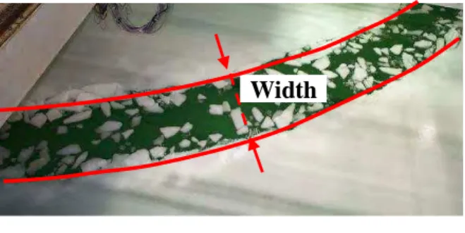
A satisfactory simulation of the geometry of the broken channel is important, as the intact ice edge interacts with the ship hull leading to interaction load (Lau et al, 2004). The hull, due to the flexural bending failure at the ice-hull contact area, breaks the unbroken ice sheet and the ice cusps are continuously created with the ship’s motions. Some the cusps of ice reach the hull bottom and leave the hull eventually and others may be pushed to the sides of the ship. A channel is cleared behind the icebreaker. The ice properties and ship’s velocities directly affect the size of ice pieces broken by the hull. The drift angle and constant radius directly affect the positions of the ice-hull contact and the shape of the ice edge the ship leaves behind. The different channel width reflects a different ice-hull contact condition that, in turn, determines the ice force distribution along the hull surface and affects the global ice forces imposed on the ship. Figure 6 shows the channel created by the Terry Fox model in a constant radius run with 0.4 m/s tangential velocity and 10 m turning radius. Figure 7 shows the channel simulated by the IHI model for the same test condition. The model calculated the average channel resulting in a smooth channel edge as shown in Figure 7. The actual ice channel edges observed during tests were irregular; therefore, trend lines were used to fit the measurements, i.e., the red curves in Figure 6, and the average width between two trend lines was used for the comparison. Figure 8 showed a comparison between the predicted channel widths and the measurements (Lau, 2006) as a function of turning radius for the Terry Fox model tests.
The comparison showed that the calculated channel widths agreed well with the measurements, i.e., they fell within 10% of each other; therefore, the simulated channel width was reasonable and acceptable. The 50 meters radius data agreed better than that of the 10 meters radius data. It might be due to the different sample size of channel width measurements, as more data points taken for the 50m runs reduced the uncertainty of the width estimate.
4.4 Ice Force Comparison
4.4.1 Resistance Tests
Figure 9 shows a comparison of the measured resistance force to its predictions for the Terry Fox resistance tests in level ice and pre-sawn ice. Again, they agree well with each other with a relative discrepancy smaller than 20% for most data points. The discrepancy may be due, in part, to uncertainty and non-uniformity of ice properties, i.e., ice thickness, ice density, failure strength, friction coefficients, etc, over the entire ice sheet.
Except for the data point corresponding to 0.6m/s ship speed, which seems not follow the data trend, the predictions are lower than measurements. This may be caused by the neglect of ice crushing at the stem, secondary cracks on some big ice cusps and frictional forces during ice sliding process on the wet surface of the hull. For the pre-sawn ice run at 0.1 m/s model velocity, a relatively bigger discrepancy can be observed. The discrepancy may also be caused by the model idealization and simplifications of the problem treatment, i.e., the simple flat-plate representation of the model hull for buoyancy calculation; the idealized ice breaking process and clearing process, ice piece pattern and ice piece size, etc.
It should also be noted that the model is based on low to median ship speed. At high speed, the submersion process of ice pieces is very complicated and an independent resistance component may not exist (Kamarainen, 1994).
4.4.2 Constant Radius Tests
Figure 10 shows a comparison of the measured moment to its predictions for the Terry-Fox constant radius tests in 40mm level ice. The comparison shows the predictions were within 20% of the corresponding measurements for the 10 meters runs. For the 50 meters runs, the data spread is relatively large and only four data points are available for comparison; nevertheless, the predictions are within the spread of the measured data.
Shi (2002) reported a drift angle of 5.6º existed for the R-Class constant radius runs. Therefore, a 5.6º drift angle was prescribed in the simulations of the R-Class constant radius runs. Figure 11 shows a comparison of the measured moment to its predictions for the R-Class runs with various constant radii that were tested in 30 mm and 50mm level ice. The comparison showed that the model predicted fairly well the yaw moment and its dependency on the turning radius. The comparison showed that the discrepancy between measurements and predictions is within 15% for the 30 mm thick ice tests and 35% for the 50 mm thick ice tests. The simulation results are larger than the corresponding test measurements, which may be caused by a larger than actual drift angle than was prescribed in the simulations, which may affect the final comparison.
4.4.3 Sinusoidal Tests
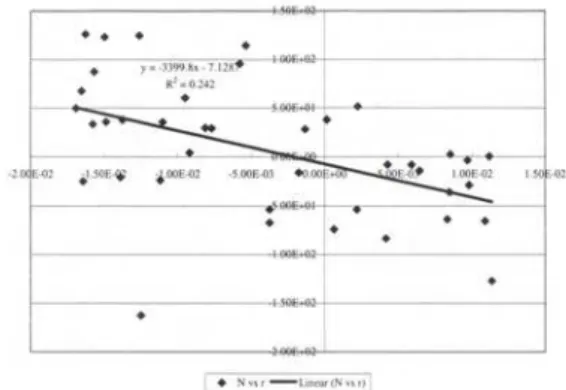
Figure 12 is the measured yaw moment measured during sinusoidal run with the R-Class model in the 30mm level ice, which were taken from Shi (2002). The runs correspond to 0.6 m/s tangential velocity100 seconds period, zero drift angle, and with a yaw rate ranging from –0.05 to 0.05 rad/s. Considering that the yaw rate kept changing in order to keep the centerline of the model always inline with its path during the sinusoidal runs, it is more practical to compare the
trend line of the measured data to that of the predictions. To compute the predicted moments, a drift angle of 0.5º was prescribed according to the measurement reported by Shi (2002).
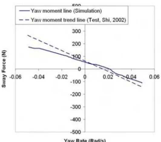
Figure 13 shows the comparison of the sinusoidal runs obtained in the 30 mm ice. Figure 14 and 15 respectively show the comparisons of the measured yaw moments and sway forces to those predicted for the 50 mm runs. The comparisons showed that the trend lines of the measured data agree fairly well to those from predictions. The simulated yaw moment vs. yaw rate curves was roughly a straight line, which was expected theoretically. The yaw moment vs. yaw rate curves and the sway force vs. yaw rate curve all offset from the origin, which may be caused by the drift angle that results in sway velocity.
It is more difficult to maintain an exactly steady sinusoidal motion in ice than in open water, andf this affected the final comparison results.
5.0 Conclusions
A new hull-ice interaction model for real-time simulation of ship navigation in level ice was presented. The numerical implementation of the model was benchmarked using data from two model test series; Terry Fox model tests and R-Class model tests, conducted at IOT using an PMM.
The benchmarking results showed the ice-hull interaction model predicted fairly well the measurements obtained from model tests with good accuracy, despite significant model idealization. The benchmarking also showed the model’s capability in simulating different ship’s manoeuvers in ice. It could favourably predict the global ice forces on the hull with good numerical efficiency and universality that are essential to marine simulation.
The comparison also showed that the drift angle played an important role in influencing the global ice loads on the hull; therefore, more attentions should be paid to the accurate control or measurement of drift angle in future tests.
Acknowledgement
This work was supported by the Institute for Ocean Technology (NRC-IOT), NSERC and the Atlantic Innovation Fund through the Modeling and Simulation of Harsh Environments Project administrated by the Memorial University of Newfoundland’s Centre for Marine Simulations. Their financial supports are gratefully acknowledged.
Reference
Derradji-Aount A., Thiel A., 2004, “Terry Fox Resistance Tests – Phase III (PMM) Testing ITTC Experimental Uncertainty Analysis Initiative”, Institute for Ocean Technology (NRC/IOT) Report, TR-2004-05.
Enkvist E. 1972, “On the Ice Resistance Encounting by Ships Operating in the Continuous Model of Icebreaking", The Swedish Academy of Engineering Science in Finland, Report No. 24, Helsinki.
Hoffmann K., 1998, “Ship Maneuvering in Ice with the Planar Motion Mechanism R-Class Testing”, Institute for Ocean Technology (NRC/IOT) Report, LM-1998-19.
Kamarainen J. 1994, “On the Speed Dependence of the Ice Submerging Resistance in Level Ice”, Proceedings of the 11th International Offshore and Polar Engineering Conference under Arctic Conditions (POAC), Osaka, Japan, pp. 578~583.
Kotras T.V., Baird A.V. and Naegle J.W., 1983, “Predicting Ship Performance in Level Ice”, Trans. SNAME, Vol. 91, New York, pp. 329~349.
Lau M., 2006, “Preliominary Modelling of Ship Manoeuvring in Ice Using a PMM”, Institute for Ocean Technology (NRC/IOT) Report, TR-2006-02.
Lau M., Molgaard J., Williams F.M., Swamidas A., 1999, “An Analysis of Ice Breaking Pattern and Ice Piece Size around Sloping Structures”, Proceedings of 18th International Conference on Offshore Mechanics and Arctic Engineering, St. John’s, Newfoundland, Canada, pp. 1~9.
Lau M., Derradji-Aouat A., 2007, “Phase IV Experimental Uncertainty Analysis for Ice Tank Ship Resistance and Manoeuvring Experiments using PMM”, Institute for Ocean Technology (NRC/IOT) Report, TR-2006-03.
Lau M., Liu J.C., Derradji A., Williams F.M., 2004, “Preliminary Results of Ship Maneuvering in Ice Experiments Using a Planar Motion Mechanism”, Proceedings of the 17th International IAHR Symposium on Ice, Saint Petersburg, Russia, pp479-487.
Liu J.C., Lau, M, and Williams F.M., 2006, “Mathematical Modeling of Ice-Hull Interaction for Ship Maneuvering in Ice Simulations”, International Conference and Exhibition on Performance of Ships and Structures in Ice, IceTech06-126-RF, Banff, Alberta, Canada (CD). Liu J., Lau, M, and Williams F.M., 2007a, “Mathematical Modelling of Ice-Hull Interaction for Real Time Simulation of Ship Manoeuvring in Level Ice”, Institute for Ocean Technology (IOT) Report: LM-2007-06.
Liu J., Lau M, and Williams F.M., 2007b, “Software of IHI Model for Simulating Ship Manoeuvring in Level Ice”, Institute for Ocean Technology (IOT) Report: LM-2007-07.
Shi Y., 2002, “Model Test Data Analysis of Ship Maneuverability in Ice”, Master Degree Thesis, Faculty of Engineering and Applied Science, Memorial University of Newfoundland, St. John’s, Canada.
Spencer D., Jones J., 2001, “Model-Scale/Full-Scale Correlation in Open Water and Ice for Canadian Coast Guard ‘R-Class’ Icebreakers”, Journal of Ship Research, Vol. 45, pp 249~261.
Jones J., Lau, M, 2006, “Propulsion and Manoeuvring Model Tests of the USCGC Healy in Ice and Correlation with Full-Scale”, International Conference and Exhibition on Performance of Ships and Structures in Ice, Banff, Alberta, Canada (CD).
Varsta P. 1983, “On the mechanics of Ice load on Ships in level ice in the Baltic Sea”, Phd thesis, Technical Research Centre of Finland, Publications 11, Espoo, Finland.
Figure 1. Global force and yaw moment calculation in IHI model
Figure 2. Software structure of IHI Model program with main m-files
Figure 3. Sketch of a flat-plate model for buoyancy force calculation
Figure 4. Terry Fox Model water line profile represented in the IHI Model
Seg.1 Xbreak Ybreak Nbreak Xbreak Ybreak Nbreak Xbreak Ybreak Nbreak Seg.2 …… Seg.1 Xclear Yclear Nclear Xclear Yclear Nclear Xclear Yclear Nclear Seg.2 …… Sur.1 Xbuoya Ybuoya Nbuoy
Breaking force Clearing force Buoyancy force
Xbuoya Ybuoya Nbuoya Xbuoya Ybuoy Nbuoya Sur.2 ……
Xice, Yice and Nice (Total ice force on whole hull) Xbreak, Ybreak, and Nbreak
(Whole hull)
Xclear, Yclear, and Nclear (Whole hull)
Xbuoya, Ybuoya, and Nbuoya (Whole hull)
Hull_ice_model
(IHI Model Core)
Param_input Motion_ship Ice_clear_force Ice_break_force Ice_buoya_force Gener_chann Calcu_conta_area Output_motion Output_force Output_chann Movie_proce Monit_calcu Others D A T A A R E A (PIL) (CCL) (ROL) α φ B T
η
I’ I II II’ Bow SternFigure 5. CCG R-Class Model water line profile represented in IHI Model
Table 1. Geometries of Terry Fox Model represented in IHI model
Location1 (m) Half WL Width (m) Flare angle (°) Area2 (m2) 3.440f 0.037 23.22 0.0705 3.096f 0.265 34.76 0.0705 2.752f 0.389 57.43 0.0883 2.408f 0.393 68.12 0.1003 2.064f 0.396 80.03 0.1248 1.720f 0.396 80.83 0.1253 1.376f 0.396 80.83 0.1254 1.032f 0.395 80.75 0.1297 0.688f 0.389 76.65 0.1236 0.344f 0.370 64.20 0.1041 0.000f 0.294 27.34 0.0969
Table 2. Geometries of IOT R-Class model represented in IHI model
Location1 (m) Half WL Width(m) Flare angle (°) Area2 (m2) 4.5257f 0.000 24.73 0.0404 4.2669f 0.1611 38.67 0.0404 4.0128f 0.294 52.56 0.0769 3.632f 0.417 50.25 0.1642 3.2504f 0.471 57.76 0.1537 2.8692f 0.483 68.33 0.1378 2.3609f 0.483 73.03 0.1710 1.7256f 0.478 73.78 0.2111 1.2173f 0.466 64.10 0.1747 0.8361f 0.426 53.20 0.1426 0.4549f 0.344 40.58 0.1234 0.0737f 0.154 28.11 0.0912 -0.0765f 0.0 35.99 0.0150 1 The transverse plane was measured at interval forwards of the aft perpendicular (AP).
2 The equivalent area of the hull side surface under the waterline till the bottom at each section as shown in Figure 3.
Figure 6. Channel left by Terry Fox model in the constant radius test run
Figure 7. Sketch of the channel width in the ship’s constant radius runs
Figure 8. Simulated and measured channel width as a function of the turning radius
Width Width
Bow Stern
Figure 9. Comparison of measured and simulated resistance for Terry Fox Model in
40 mm - 31.5 kPa ice at test speeds ranging from 0.1 to 0.6 m/s
Figure 10. Yaw moment comparison for Terry Fox Model with 10 and 50 meters
radius turning in 40mm-31.5kPa ice
Figure 11. Yaw moment comparison of IOT R-class Model constant radius runs in 30
mm-20 kPa and 50 mm-20 kPa level ice
Figure 12. Regression test results of R-Class model sinusoidal run in 30 mm - 20
kPa level ice (Shi, 2002)
Figure 13. Yaw moments comparison of R-Class Model sinusoidal run in 30 mm - 20
kPa flexural strength ice.
Figure 14. Yaw moments comparison of R-Class Model sinusoidal run in 50 mm - 20
kPa flexural strength ice Erratic point
Figure 15. Sway force comparison of R-Class Model sinusoidal run in 50 mm - 20