A Biologically Motivated Paradigm for Heuristic
Motor Control in Multiple Contexts
by
Max Berniker
Submitted to the Department of Mechanical Engineering
in partial fulfillment of the requirements for the degree of
Masters of Science in Mechanical Engineering
at the
MASSACHUSETTS INSTITUTE OF TECHNOLOGY
September 2000
©
Massachusetts Institute of Technology 2000. All rights reserved.
A u th o r ...
Department of Mechanical Engineering
August 4, 2000
Certified by..
V\
Neville Hogan
Professor
Thesis Supervisor
Accepted by ...
...
Am Sonin
Chairman, Department Committee on Graduate Students
MAS SAC HUSESTrSNiTUTE
OF TECHNOLOGY
SEP
2 02000
~2~N
A Biologically Motivated Paradigm for Heuristic Motor
Control in Multiple Contexts
by
Max Berniker
Submitted to the Department of Mechanical Engineering on August 4, 2000, in partial fulfillment of the
requirements for the degree of
Masters of Science in Mechanical Engineering
Abstract
A biologically motivated controller is presented and investigated in terms of motor
control and motor learning, especially motor learning of different behaviors. The controller, based on several ideas presented in the literature, used multiple paired inverse and forward internal models to generate motor commands and estimate the current environment within which the controller operated. The controller demon-strated an ability to control a simulated arm-like manipulator making 20cm reaching movements with an RMS position error of 4.6mm while making unperturbed move-ments, and 6.40mm while making the same reaching movements within a curl field. However, the ability to learn and retain multiple motor behaviors was proven not to be possible with the current paradigm and its learning algorithm. The results of the investigation were viewed in the scope of motor control for engineering purposes, and for use in developing a model for human motor control to further the science of neuro-recovery.
Thesis Supervisor: Neville Hogan Title: Professor
Acknowledgments
I would like to start by thanking my advisor, Neville Hogan. I am very grateful for all that I have learned from him. His analytical skills, technical knowledge and practical know-how combine to rattle off insightful gems at a machine gun pace -it's something to behold -it's inspiring. Truly, it was an honor to work under him.
As always, in life as well as work, it's the people you share it with that make for especially memorable and valuable experiences, ...so I'd like to give a shout-out to all my hommies in the mezzanine! I'd like to thank Steve, one sharp kid who taught me the correct use of a semicolon; it's the little comma looking-thing you place between to complete sentences. I'd like to thank Brandon, for always allowing me to use him as a sounding board. His sage and thoughtful advice were always helpful. I'd like to thank Brian for enlightening me as to the ways of the farm (and big-city dating techniques). And Patrick and Keng, despite their spoiled Hunter lab background, are a welcome addition to any up-and-coming boy band (373K baby!).
I would also like to thank the members of Neville's research group, Dustin, Kris,
Jerry and especially Lori and Igo, for all their support in my studies.
Of course, I must thank my team, "Newman's Neanderthanls", a rag-tag band
of misfits that I singlehandedly whipped into an unstoppable hockey machine! John, Peter, James, Bobby D., Tanya, and our golden boys, Verdi and Matt. They would make any captain glow with pride.
I'd also like to thank one of our fallen mezzanine members, Luke Sosnowski, no
longer with us, he will forever work in the mezzanine of our hearts.
I owe a great debt to Robin (you know who you are). Thanks honey-bunch.
And finally, I would like to thank the lovely ladies of the mechanical engineering graduate office, Leslie Regan and Joan Kravit. I believe that they, more than anyone else in the department, are responsible for making graduate studies at MIT a more
"human" experience.
This work was supported in part by NIH Grant R01-HD37397 and by the Winifred Masterson Burke Medical Research Institute.
Contents
1 Introduction
2 Human Motor Control
2.1 Organizing Models: A Search For Invariants 2.1.1 Kinematic vs dynamic based models 2.2 Equilibrium Point Control Hypothesis . . . . 2.3 Inverse Dynamics Model Hypothesis . . . . .
2.4 Conclusion . . . . 13 19 . . 20 . . 21 . . 23 . . 26 26 3 Networks 3.1 Neural Networks . . . 3.2 Training Algorithms 3.3 Training Paradigms 3.4 Dimensional difficulties 4 Physical Apparatus 4.1 Physical Model . . . . 4.2 Mechanics . . . . 4.2.1 Kinematics . . 4.2.2 Dynamics . . . 4.3 Motor Commands . . .
5 A Motor Control Paradigm
5.1 Internal m odels . . . . 29 . . . . 2 9 . . . . 3 2 . . . . 3 3 . . . . 3 8 39 . . . 39 . . . 40 . . . 40 41 . . . 41 45 46
5.1.1 Forward models . . . . 46
5.1.2 Inverse models . . . . 47
5.2 The Control Paradigm . . . . 47
6 Experiment 57 6.1 Objectives . . . . 57 6.2 Overview . . . . 57 6.3 Procedure . . . . 59 7 Results 61 7.1 Physical Parameters . . . . 61 7.2 Network Tuning . . . . 62 7.3 Kinematic Models . . . . 63
7.3.1 Forward Kinematic Model . . . . 63
7.3.2 Inverse Kinematic Model . . . . 65
7.4 Dynamic Models . . . . 67
7.4.1 Forward Dynamic Model . . . . 67
7.4.2 Inverse Dynamic Model . . . . 73
7.5 Experimental Results . . . . 77 7.5.1 Tasks 1 and 2 . . . . 78 7.5.2 Task 3 . . . . 82 7.5.3 Task 4 . . . . 86 8 Discussion 91 9 Conclusions 105 9.1 Review . . . . 105
9.2 Recommendations For Future Work . . . . 106
Appendix A Two-Link Dynamics 111
Appendix C Lyapunov Stability
Bibliography 121
List of Figures
3-1 Diagram of Radial Basis Function Network . . . . 31
3-2 Schematic representation of supervised learning. . . . . 34
3-3 Schematic representation of direct inverse learning. . . . . 35
3-4 Schematic representation of distal supervised learning. . . . . 36
4-1 Diagram of arm-like manipulator. . . . . 40
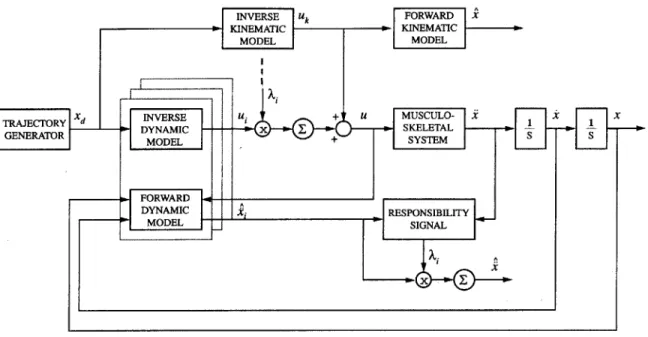
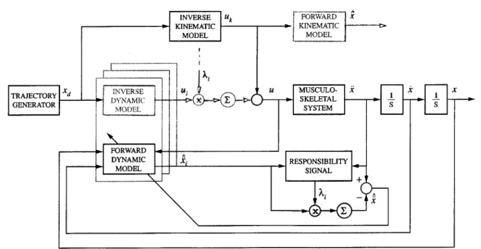
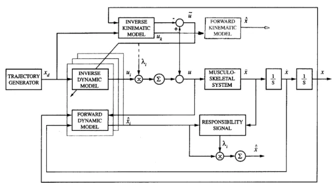
5-1 Diagram of control architecture. . . . . 54
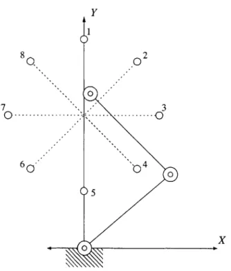
6-1 Diagram of target geometry . . . . 58
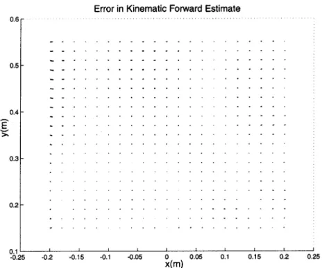
7-1 Error in forward kinematic estimate of endpoint coordinates. . . . . . 65
7-2 Error in inverse estimate of endpoint coordinates. . . . . 66
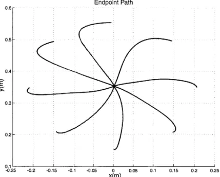
7-3 Resulting path of endpoint in unperturbed context. . . . . 68
7-4 Resulting path of endpoint in curl field . . . . 68
7-5 Path of end point in curl field . . . . 69
7-6 Diagram of control system while training the forward dynamic models. 70 7-7 Forward estimate of the x component of the acceleration of the end-point with 729 nodes . . . . 72
7-8 Forward estimate of the y component of the acceleration of the end-point with 729 nodes . . . . 72
7-9 Forward estimate of the x component of the acceleration of the end-point with 4,096 nodes . . . . 74
7-10 Forward estimate of the y component of the acceleration of the end-point with 4,096 nodes . . . . 74
7-11 Diagram of control system while training the inverse dynamic models. 76
7-12 Endpoint path after approximately 150 training sessions . . . . 77
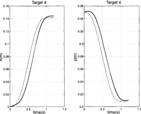
7-13 Large acceleration due to boundary layer dynamics, x component. . 79 7-14 large acceleration due to boundary layer dynamics, y component. . 79 7-15 End point path, x component. . . . . 80
7-16 Diagram of shaped steps used for training the inverse dynamic models 82 7-17 RMS acceleration of the endpoint for various shaped steps, x component. 83 7-18 RMS acceleration of the endpoint for various shaped steps, y component. 83 7-19 end point path for task 1 . . . . 84
7-20 End point path for task 2 . . . . 84
7-21 Average responsibility signals for task three . . . . 86
7-22 Endpoint path in context one using module one . . . . 87
7-23 Endpoint path in context two using module two . . . . 87
7-24 Average responsibility signals for task three . . . . 89
7-25 Endpoint path in context one using module one . . . . 89
7-26 Endpoint path in context two using module two . . . . 90
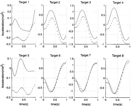
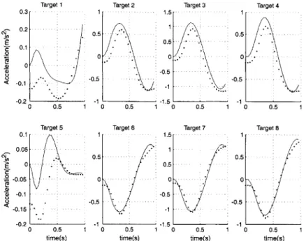
8-1 Endpoint acceleration, x component. Solid lines represent interaction in context one, dotted lines are context two. . . . . 93
8-2 Endpoint acceleration, y component. Solid lines represent interaction in context one, dotted lines are context two. . . . . 93
8-3 Mean responsibility signal during new task 3 . . . . 95
8-4 Varying responsibility for varying x. . . . . 101
Chapter 1
Introduction
Science and technology exist in such highly evolved states today as to approach most technical problems in exceedingly complex manners. But perhaps more elegant solu-tions exist -solusolu-tions that do not rely on precise physical representasolu-tions and brute force computation, but rather insight into natural processes that have already skill-fully met the challenge. Many of the technical problems we face have parallels in nature. Biomimicry and a search for parallels in nature for these technical prob-lems are gaining a broader acceptance. By inspecting nature for similar probprob-lems and examining the solutions to these natural systems, an otherwise untapped source of inspiration for strategies in our technical solutions are offered. A wise choice in confronting engineering problems might be to seek out appropriately similar natu-ral systems; do they have similar goals and/or objectives to our current problem?
By examining the solutions to these parallel systems we can identify what, if any,
characteristics these natural systems have that might be practical or pragmatic for emulating.
From an engineering standpoint people represent excellent control systems. In homage to the competence of this natural machinery they have been emulated time and time again in one form or another, from factory floor automation that bears a striking functional resemblance to a human arm, to neural networks that mimic human minds in their calculations, to robots, made in man's image.
compare with humans and other biological entities? Certainly they are marvelous tributes to science and the technology that drives it. Generally speaking, machines can be built for a particular task to move faster, stronger, longer and more accurately than any person or animal ever will. Yet they usually are built to perform this very specific task. Their ability to perform outside the scope of their intended context is limited. Often a great deal of a priori knowledge is required as well. The machine must be given rules and guidelines for all the decisions it will be faced with concerning its task and the environment therein. If and when the machine's knowledge of its environment is lacking, failure is likely.
Humans on the other hand are endowed with an enormous capacity for varying tasks. Grasping, reaching, walking, running, dancing; the list of behaviors humans can exhibit goes on without end. An equally obvious observation is the ability we possess to quickly adapt to unknown tasks by generalizing previously learned knowl-edge and skills; learn to juggle and one can easily conquer the task while walking as well. The capacity for retrieving learned behaviors when confronted with unknowns and adapting in a timely and stable fashion is so commonplace, indeed so second na-ture, that one barely takes note of the remarkable motor control and motor learning
involved.
This is where we as humans tip the scales on performance next to our man-made machines and the intelligence (or lack thereof) that controls them. Our aptitude for interacting through our bodies with unknown environments or contexts, as they shall be referred to, is a challenge that is poorly met by our man-made counterparts. These contexts represent a continuum from the completely unknown to the completely known. This is testament to the robust motor control and motor learning abilities that humans are equipped with.
Reaching for an object is no difficulty for a normally functioning human. A robotic arm can be made to execute the same task. Depending on the level of performance desired and the knowledge required for the task, a considerable amount of time and effort might be devoted to computing the proper chain of events that would lead to a successful grasp. When reaching for the same object through a viscous fluid,
highly nonlinear forces difficult to quantify will perturb your arm. You are compelled
to compensate. Yet again the task represents little to no difficulty for a human. How does the robotic arm fare? The same task, yet the environment or the context within which the robot arm is operating has changed. The required actions necessary will be considerably different for the robotic arm now. This same task performed in a different environment will be referred to as a new behavior. For the robotic arm the two behaviors represent interactions within different contexts that require different sets of rules. It would further require some way of determining when to act according to which set. Humans must also cope with these problems, problems of motor learning, though apparently without difficulty.
How does the human motor control system work? It is not completely under-stood. There is a great deal of evidence to support the claim that humans generate the actions necessary for motor control based solely on experience and models built of this experience. In some sense it could be argued that one does not require ex-tensive intelligence if one has an exex-tensive memory. Internal models learned through empirical data can in theory allow an empty substrate to gain a working picture of its environment without any a priori knowledge. Simply through an elaborate scheme of trial and error, models can be built that help to describe unknown processes. For instance, if one merely remembered every task performed and all the necessary bits of information that one would require to reconstruct that task (the actions taken and the resulting outcomes) then new tasks could be adapted to according to previ-ously experienced ones. These learned internal models allow for informed actions and insight when encountering unknown contexts.
So it appears nature has provided an inspirational example for motor control and motor learning in ourselves. Whether or not this biological system will prove beneficial to emulate remains to be seen. The first step though is to investigate how we manage these worthy qualities, motor control and learning. With the human system as a prototype, control systems may be designed that complement human control aptitudes with current control theory for increasingly sophisticated technical solutions.
The benefits of emulating human-like motor control and motor learning may not be limited to better control systems. With a clearer understanding of human motor control and motor learning we are in a position to make more effective decisions concerning these aspects with regard to our health. With human motor control understood in the context of engineering control systems, well traveled analysis tools may be employed for insight into the human system and any problems that may arise within it. This could be beneficial not only in the treatment of human pathologies, but also for extending normal human capacities.
Recently studies have provided evidence to suggest that robot-aided therapy can be of assistance in the rehabilitation of individuals with neurologic injuries. It is an auspicious augmentation to the time-honored rehabilitation process of a therapist and patient manually working the impaired limbs and limb segments. It is not unreason-able to suspect that, with a deeper understanding of the mechanisms behind human motor control, this rehabilitation process can be made more effective.
A model of the human motor system would be useful in this regard. The model
might elucidate the processes that underly the human system. For instance, a promi-nent question concerning human motor control is whether or not recovery (from neu-rologic injury effecting motor control) is similar to motor learning. With such a model this question could be addressed. Similarly, different rehabilitation procedures could be quickly evaluated in terms of their efficacy and expediency by determining how they would interact with a model that emulates human motor control.
This thesis seeks to explore current theories concerning human motor control and motor learning in an effort to emulate these mechanisms. The goal is to examine a biologically motivated controller as a means to intelligent, modular and hierarchical control with a heuristic approach to learning multiple behaviors and a method for retrieving them when appropriate.
The controller consists of multiple paired, forward and inverse models. Forward models help to estimate the current context within which the controller is interacting. Inverse models are used to generate motor commands. With multiple paired models the controller should be able to store learned behaviors for different motor tasks and
still adapt to new behaviors without sacrificing those previously learned. Utilizing neural networks the models are built upon the experience gained through interacting within different contexts. A method for switching between the learned behaviors based on sensory feedback is presented. The controller is used to mimic the movements of a human arm. To this end a human-like arm is simulated with anthropomorphic data and anatomical principles.
Two questions will be addressed: Is the controller a useful control alternative? And does the controller shed light onto the field of human motor control? In order to explore the utility of this control system, an experiment was devised that would investigate its ability to learn and retain new behaviors, the prudence to call upon this information when appropriate, and the insight to use these tools in unknown situations. Should the controller exhibit these abilities, it will have proven to display similar qualities as the human motor system. To address the question concerning human motor control, the results of a similar experiment conducted with human subjects will be compared with the results found here in order to draw conclusions about the controller and its possible similarities with its human counterpart. Should the controller exhibit these similarities, it can be investigated further to help analyze human motor control.
In the chapters that follow pertinent information for the motivation of the research work will be presented. Chapter two will discuss what is thought to underly the hu-man motor control system in an effort to better describe the approaches taken in this thesis. Chapter three is a brief introduction to neural networks, key to implementing the controller. Chapter four presents the simulated physical apparatus upon which the experiments are conducted. Chapter five will present the control paradigm under investigation. Chapter six will explain the experiment tasks to be completed and the remaining chapters shall cover the experiments conducted and the results found.
Chapter 2
Human Motor Control
This thesis is concerned with the mechanisms by which humans generate motor control and motor learning in terms of conventional control systems engineering. With that objective in mind the next step should be to analyze human motor control. This poses a respectable problem. Psychophysical systems, including the human one, are notoriously difficult to analyze in a traditional engineering sense. Even the simplest of behaviors involve a great number of nonlinearities and redundancies that make characterization intractably difficult. For instance, the act of maintaining an arbitrary posture, arguably the most fundamental of human motor behaviors, can represent a staggering number of modeling difficulties. Take the human arm, seven degrees of freedom (not counting the hand) making it kinematically redundant. Over 26 muscles actuate the arm, each highly nonlinear and exceedingly difficult to parameterize. The forces they impose on the skeleton depend on the configuration of the arm. Communication between the central nervous system and these muscles is conducted through a great number of descending and ascending neural pathways. Where does one begin? Attempting to model the complete system would be an effort made in vain. The conclusions drawn from such a highly complex model would be dubious at best.
In contrast to the problems facing this bottom up approach to analyzing the hu-man motor system, taking a top down approach has made great strides. By examining the large picture one does away with the need to model and analyze the finer details.
Instead the focus is broadened and notice is brought to bear upon global features. Concerning human motor control, a wise course taken in the past has been to observe natural human phenomena for patterns.
2.1
Organizing Models: A Search For Invariants
Throughout the great majority of normal human movements there are several pat-terns. Work done by Morasso [25] in analyzing human reaching movements revealed two kinematic invariants. Human reaching movements tend to be straight with re-spect to the hand and have a characteristic bell shaped velocity profile. These features are only found when measured in a fixed Cartesian reference frame. Similar invari-ants could not be detected for the angular components of these reaching movements. These smooth hand trajectories were observed with such consistency that investiga-tors proposed that the central nervous system might plan movements with respect to the motion of the hand and worked to quantify this behavior.
Hogan [14] found that in the single degree of freedom case these kinematic invari-ants could be explained assuming the central nervous system organizes movements such as to optimize the smoothness of the hand's trajectory (assuming normal unper-turbed reaching movements). To derive an analytical expression for describing these movements an appropriate cost function was formed. The smoothness was defined as the mean squared jerk integrated over a reaching movement. Utilizing optimiza-tion theory to minimize this funcoptimiza-tional results in a quintic polynomial for the hand's trajectory. Imposing the appropriate boundary conditions this minimum jerk profile (the quintic polynomial) was found to agree fairly well with experimental data. This idea was then extended to the multi degree of freedom case by Flash and Hogan [8]. It was found that similar conclusions could be made by minimizing the mean squared jerk in Cartesian hand coordinates 1.
Similar attempts were made to characterize human reaching movements in terms
an analogous polynomial can be obtained by minimizing jerk in joint coordinates but the result-ing hand trajectories vary considerably from actual hand paths further supportresult-ing the claim that the central nervous system plans movements in hand coordinates
of "effort". Uno et al. [33] made use of similar optimization principles by minimizing the integral of the time derivative of torque. The resulting expression describing the torque necessary for a smooth movement captured the experimental data as well. A similar level of success was to be expected for the single degree of freedom movements though, for in the single joint case the time derivative of torque and jerk (the third derivative of position) differ by a scaling factor, the inertia of the limb. The ideas were extended to the multi-degree of freedom case but with less success
2.1.1
Kinematic vs dynamic based models
The work of Hogan and Flash carries with it some distinct and fortunately quantifiable implications. If human movements can be typified merely by minimizing a derivative (the third time derivative) of a coordinate based variable then what can be said of the organization of movements? Clearly if this is all the information the central nervous system incorporates, then movements must be organized kinematically. Some definite predictions for a kinematic based model can be inferred for motor control. Perceived errors in the hand trajectory should elicit corrective motor commands. This means that for varying conditions varying motor commands would be required for the same trajectory.
A further implication of the kinematic model lies in the progression of neural
events that conclude in motor commands. Once a kinematic trajectory has been fashioned (based entirely on kinematics) the appropriate motor commands must in turn be generated. The presumption here is a hierarchy underlying the organization of movement -kinematics and then dynamics.
The work done by Uno, Kawato and others pursuing this same line of ideas carries its own implications as well. If human movements can be typified by minimizing a derivative of a force variable (first time derivative) the underlying organization must be dynamic in nature. In contrast to the kinematically organized model, a dynamically organized model that perceives errors in the hand trajectory, provided
2
A closed form solution is not available in the multi degree of freedom case and iterative methods
they do not alter the desired terminating state, will elicit no motor response.
Continuing the comparison between the two models, consider the progression of neural events that must take place when movement is organized with a dynamic based model. Whereas the kinematic based model must tackle the distinct steps of trajectory formation and corresponding motor command generation, the dynamic organization of movement results in explicit motor commands. There is no need for separating the organization of motor planning and the resulting motor commands into two distinct processes.
Proponents of both camps have sought to provide evidence for these two opposing concepts regarding motor control. As mentioned previously, kinematically organized movement does not take into consideration the forces required when creating hand trajectories. If human movements are organized as such, then perturbed hand paths would elicit motor commands such as to return the hand to its desired trajectory. An experiment was designed to test this exact deduction (Wolpert et al. [35]). Partici-pants were asked to make point to point movements while the position of their hand was displayed to them via a monitor. While the trials took place their hand path was visually perturbed so as to appear more curved than was the case. The participants almost invariably compensated for the perceived perturbation.
Many similar experiments have been performed with curl fields ([5, 11]). Partic-ipants (both primates and humans) were instructed to make normal reaching move-ments to displayed targets. A velocity dependent force tending to curve their hand paths was applied. Just as in Wolpert's experiments, subjects always displayed a marked level of adaptation so as to straighten their hand paths. What these studies have shown, is the propensity humans have to produce straight line hand paths, even when perturbed such that forces in excess of those normally required are necessary.
It should be noted that the kinematic based model makes no claims about the process of generating motor commands. It solely claims to describe the underpinnings of the organization of movement. The dynamic model on the other hand offers a solution by predicting the necessary forces for a movement.
2.2
Equilibrium Point Control Hypothesis
An early theory concerning the generation of motor commands proposed by Feldman
[7] stated that neural activity, descending and ascending pathways and peripheral spinal loops, whose aggregate response was tantamount to specifying an equilibrium configuration, initiated movement. This idea, termed Equilibrium Control, is an attractive proposition in the light of a kinematic based model. So whereas the issue of motor commands is somewhat circumvented with the kinematic based model for the organization of movements, when combined with equilibrium control a plausible solution surfaces.
If motor commands are in effect attractors within muscle space (the space
repre-senting muscle lengths), allowing the limb to tend to an equilibrium configuration, then movement might be initiated by varying this equilibrium configuration to corre-spond with a desired hand trajectory. The inherent stiffness properties of the neuro-muscular system might then provide an adequate form of closed loop feedback about this trajectory. This means that the central nervous system might (at least for normal reaching movements) require little or no knowledge of the dynamics involved therein. To help place this into perspective a review of some of the basics of the neuro-muscular system is in order. As previously stated the properties of muscle are highly non-linear. The force they generate is a function of a pool of neural activity, their resistance to deformation (stiffness) and deformation rate (viscosity). Yet there is a degree of design in place that makes for some sound simplifications.
For a fixed level of activation muscles exhibit characteristic tension vs. displace-ment and tension vs. displacedisplace-ment rate curves. Although these dependencies are nonlinear they nonetheless attribute a visco-elastic property to muscle. Peripheral reflex loops also elicit a spring like quality. The stretch or myotatic reflex is elicited through a relatively simple loop of neural activity. When muscle stretches intrafusal muscle spindle fibers are excited. These neurons form a feedback loop with efferent alpha motor neurons whose activity is responsible for stimulating muscle. When al-pha motor neurons fire they in turn excite gamma motor neurons. These gamma
motor neurons innervate the muscle spindle fibers and through their activity effec-tively change the null point of the spindle fibers response. In a normally functioning person this all contributes to a relatively fast reflex loop allowing for corrective forces when the muscle is perturbed.
A complete description of the neurophysiology of the neuromuscular system is
beyond the scope of this thesis. Suffice it to say that the aggregate behavior of the muscle and this peripheral reflex loop is like that of a controllable, damped spring. A spring's resistance to stretch is a conservative force. The energy stored in a deformed spring (linear or non-linear) or any collection thereof can be represented by a potential function. Furthermore, potential functions by definition have zero curl. Therefore you would expect that if the human body, or in particular the human arm, could be represented by a collection of springs then a potential could be found for it with zero curl.
Several such experiments have found this to be fairly true under particular con-ditions. Shadmehr et al.[31] and Mussa-Ivaldi et al.[26], measured the postural hand stiffness of human subjects and found that the stiffness tensor was virtually curl free. With spring-like muscles, somewhat analogous to proportional-plus-rate control, the human system is equipped with instantaneous corrective forces when perturbed from its intended trajectory. More support for this notion can be found in the per-formance characteristics of human movement.
Descending cortical motor signals have a transmission delay of approximately 100 ms. Peripheral spinal reflex loops have a transmission delay of approximately 30ms (for the upper limb). By some estimates these transmission delays would put a limit on the effectiveness of any control based on feedback at around .5Hz (one twentieth of the inverse of the transmission delay). However many human movements exhibit frequency components of up to 15Hz [18]. Muscle stiffness then offers a plausible explanation for the bandwidth of human movements;3 the intrinsic elasticity, damping
and peripheral reflexes act as an internal feedback loop.
3
the redundancy of the human musculature in the form of agonist and antagonist muscle pairs, also play a critical role in this elasticity
Returning to the equilibrium control hypothesis we see that combined with muscle elasticity and a kinematically organized movement strategy motion can be produced
by an appropriate set of neural commands such as to shift the equilibrium point of
the neuromuscular system. Motor commands constructed in such a way entail little more than a mapping from a desired equilibrium configuration to an appropriate set of neural commands.
Experiments conducted on spinalized frogs [3] provided some interesting and ap-parent support for an equilibrium point control scheme. By stimulating distinct neurons in the spinal cord, groups of muscles could be activated whose coordinated contractions generated a force field about an equilibrium point in space. What is more, it was found that when stimulating two sites simultaneously the resulting force field was the vector sum of the individual respective fields. The natural conclusion seems to be that the central nervous system can define any equilibrium posture, pro-vided it can be composed by a superposition of these discrete equilibrium points, by conjointly varying the activation of the respective spinal neurons.
Further evidence was found in the work done by Flash in human reaching move-ments [9]. She demonstrated how by merely modeling the muscles of the arm as linear springs and dampers in parallel and the descending neural signals as equilibrium joint motor commands, she was able to produce hand trajectories that agreed remarkably well with experimental data.
The advantages of an equilibrium point (EP) control hypothesis, combined with a kinematic strategy for motion and elastic muscles, are twofold. Such a strategy provides a means to generate motor commands, and implies a relative ease of neural computation required. It should be noted here that any conjecture as to what the central nervous system and the brain find difficult to compute is simply that, conjec-ture, but provided the relative difficulty of neural computation is analogous to the relative difficulty of conventional computation there are some advantages. If descend-ing motor commands correspond to a time varydescend-ing equilibrium arm configuration or a virtual trajectory [14], then this at least in part alleviates the need for precise es-timates of inertial and viscous parameters should an inversion of the dynamics be
needed.
2.3
Inverse Dynamics Model Hypothesis
Another prevalent theory concerning the initiation of movement asserts that while the central nervous system must proceed from a kinematically defined trajectory to limb motion, it is done by inverting the dynamic equations of the limb to compute the necessary muscle forces. In contrast to the equilibrium control hypothesis, this would require precise estimates of the inertial, viscous and stiffness parameters of the limb.
Investigating the use of internal models Gomi et al.[12] criticized Flash's work asserting that the muscle stiffness values she used were too high. Flash's simulations of reaching movements were based on a two-link manipulator model of the arm. The stiffness and damping values representing the muscles behaved as a proportional-plus-rate controller. No further assumptions are necessary to conclude that provided the arm isn't excited at resonance, higher gains (stiffer muscles) will translate to better trajectory following. Gomi and Kawato measured arm stiffness on separate occasions and found the numbers to be much lower than those used by Flash.
2.4
Conclusion
There is a great deal of support for kinematically organized movements that corre-spond to straight line hand paths with bell shaped velocity profiles. These movements might be controlled via an equilibrium point. Following a virtual trajectory in mus-cle space based entirely on the desired trajectory, elastic musmus-cles might account for movement. This hypothesis might decrease the amount of computation necessary for the central nervous system, but it is lacking in some regards. The values needed for muscle stiffness to account for the trajectory following observed are in question. The support for the inverse dynamics model, wherein motion is created by inverting the dynamics of the arm to generate the forces necessary to follow the desired trajectory,
is not as strong. But it too has some attractive qualities. If the central nervous system were to incorporate the dynamics involved in motion for the creation of motor commands, then low muscle stiffness might be reconciled.
Chapter 3
Networks
3.1
Neural Networks
Neural networks are fundamental to the work presented in this thesis. As a result, some effort in explaining the material is in order. First and foremost, what are neural networks? By one author's definition,
"A neural network is a massively parallel distributed processor that has
a natural propensity for storing experiential knowledge and making it available for use.1"
Neural networks, or more simply networks learn mappings. In their most fun-damental interpretation they are a method of function approximation. They can be considerably sophisticated or considerably commonplace. In addition to their re-spectable utility they carry a commensurate number of allusions to intelligence, both of the machine and biological sort. For the purposes of this thesis though, the analogy of networks with supposed mechanisms of biological intelligence is only an interesting and perhaps insightful footnote. This is not meant to dismiss any value that neural networks might have in deciphering biological intelligence. On the contrary, there is much to be gained through the analogy. This is only meant as a qualifying statement concerning the goals of this research. For although neural networks fit nicely into
the current framework of a biologically inspired control architecture, they are of most benefit as a robust and heuristic approach to function approximation.
Regression is an attempt to estimate a function from some example input-output pairs. The distinguishing feature of non-parametric regression is that there is little or no a priori knowledge of the form of the true function. For example, if the relation
y = f (x) (3.1)
is to be estimated, nothing needs to be known of the nature of
f.
The estimate is formed through use of a model#
such thatS= O(x) (3.2)
The form of the model
#
arises while attempting to match the example input-output pairs. Networks are non-parametric models. Based loosely on the structure of the central nervous system, they normally consist of a group of simple processing elements referred to as nodes, which are analogous to neurons. These nodes have a large interconnected topology such that there is a great deal of interaction between them. The resulting activity of any individual node is a function of the weighted inputs of the nodes connected to it.Traditionally networks have been organized into layers wherein each layer receives input from the one before it and projects its outputs to the one ahead of it. These multi-layer feed-forward networks have the capability of learning any function within arbitrary accuracy, provided they have at least three layers. More layers may be useful for functions that contain discontinuities or similar pathologies.
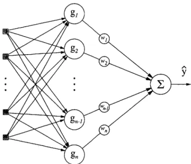
One particularly alluring class of networks is the radial basis function network, or RBF network. An RBF network is a single-layer linear model (figure3-1), hence the mathematics are relatively simple. As a result, linear optimization tools may be employed when desired. It has also been demonstrated that while multilayer networks have the ability to approximate arbitrarily well any continuous function, RBF networks have similar properties and map directly onto this class of three-layerered network. Unlike the nonlinear multi-layer networks, the RBF network does
w
Wn
gn
Figure 3-1: Diagram of Radial Basis Function Network
not face the same difficulties with local minima that hamper traditional multi-layer network training.
An RBF network is so named for its basis functions. Radial basis functions mono-tonically decrease (or increase) away from a center. The basis function most often used, and the one used in this thesis, is the Gaussian. The GRBF (Gaussian-RBF) network is a linear sum of these weighted Gaussian basis functions. By adjusting the weights associated with individual basis functions the model "learns" the unknown function. This is the process of training. Unlike conventional feed-forward networks where the output is a nonlinear function of the varying weights the GRBF network is a linear summation of nonlinear basis functions. The resulting model q has the form:
(X, W)- n - - ,)2
(x, 'w) = $ wigi (x) where gi(x) = exp 2 (3.3)
i=1
where i and a? are the center and variance of the it" basis function.
The GRBF networks are analogous to a nonlinear form of signal reconstruction. Instead of using a sample-and-hold scheme, which can be thought of as a series of step functions scaled by a sampled value, we use Gaussians and scale them to most closely match the sampled signal. Moreover, because the Gaussians are a function of
the input variables, an estimate of the true function can be built. Using similar ideas, Sanner and Slotine [29, 30] derived some elegant methods for defining error bounds when using these networks.
3.2
Training Algorithms
Training a network can be accomplished by minimizing the error between its estimated value and the desired, or true, values. Given a training set of input-output pairs,
T = {xi, yi} i a cost function is defined. For instance, the sum of squared differences
between the true outputs and the network's response given the corresponding input:
1 P
E = _ (yi _
Qi)2
(3.4)2i=1
The goal is to minimize this cost function over the training set. To do this we need to express how each weight in the network contributes to the error functional so that the weights can be adjusted accordingly. This is done by back-propagating through the function E to compute the gradient. Taking the partial derivatives of E with respect to the weights we have:
V,,E = -
a
(yi - Vi) (3.5)Thus the gradient is computed by multiplying the error by the transpose of the Jacobian matrix, OQT/&w. This expression describes a vector (in n dimensional space where n is the number of weights) pointing in the direction of greatest increase in the cost function, or the error. To reduce this error the weights are moved in the opposite direction. This is the basic description of a gradient descent training algorithm; evaluate the Jacobian at the current x and increment the weights in proportion to the current error. Fortunately, computing the Jacobian of the GRBF network is relatively easy because of the linear nature of the network (Appendix A). Other approaches of varying levels of sophistication can be taken as well.
The gradient descent algorithm is well suited to an "on-line" learning scheme, where on-line describes an iterative routine of incremental adjustments to the network at each sampling cycle. With this approach, there is no training set to start with and
training pairs are measured at each sample. The training set will then consist either of a single training pair or a running tally of training pairs constituting a growing training set. The weights are adapted each training cycle by computing the gradient and adjusting with some step size a as follows:
wi = wi - aVwE (3.6)
One of the major hindrances to learning is the problem of local minima. A con-ceptual construct to help visualize the way in which the error changes as the weights vary is an error landscape, similar to a potential energy landscape. While traveling through this error landscape of the cost function a gradient descent algorithm may become "stuck" within a relatively flat area of the terrain where the gradient is small or zero. This is an especially difficult problem with nonlinear networks. Fortunately, this is not the case with the linear GRBF network. The weights modulate the net-work's response in a linear fashion and therefore do not introduce multiple minima.
A further complication to training is the concept of over-training. Once the
net-work has been trained on the data set T, it should be validated. The network's response at previously untrained data points is compared with the corresponding true values. An overtrained network will give estimates within defined tolerance at the trained points but unsatisfactory estimates at these validation points. Without knowledge of the precision capabilities of the network to guide training, judging when a network has been sufficiently trained to yield a globally optimal solution is difficult.
Generally this problem is solved through trial and error.
Because GRBF networks are linear they can also make use of linear optimization tools. A least squares solution can be obtained for the optimal weight vector of a given training set. This approach can be used on-line as well, but in order to be effective a large training set is necessary.
3.3
Training Paradigms
Algorithms describe systematic steps to be taken towards solving a problem. Paradigms describe the manner in which you pose the problem to obtain a desired solution. The
x
y
-- TEACHERpo
SLEARNER
Figure 3-2: Schematic representation of supervised learning.
algorithm presented above, the gradient descent, is a tool for training networks. The paradigms explain how to use these tools. The choice of a paradigm may appear to be a trivial step, but it can make a significant difference in training a network.
Supervised learning is characterized by training with a teacher. The teacher
pro-vides correct answers to the learner, or regression model, in an effort to help it learn
by example. The input x is made available to both the learner and the teacher. The
teacher then provides the correct response, completing the training pair. The learner, while adapting according to the methods outlined above, is modeling the teacher (fig-ure 3-2). Supervised learning is especially useful when the learner is a forward model.
Forward models learn the causal relationship between inputs and outputs or actions
and outcomes.
Training an inverse model is more difficult. The inverse model, equation3.7
i = 0(y, v) (3.7)
learns to predict the action for a given outcome. In this case it learns the correct
input x, for a given output y. Often though, the correct action for a given outcome
is unknown (e.g. the forward relationship might be many-to-one and not invertible). For example, with the arm of the experiment, the forward map from joint to endpoint coordinates is many-to-one, the corresponding inverse map, from endpoint to joint coordinates is one-to-many. In instances such as this, the inverse model works most
x
y
---- TEACHER
A
+ X
(W LEARNER-*----J
Figure 3-3: Schematic representation of direct inverse learning.
efficiently when estimating a subset of the inverse mapping.
There are several approaches to training the inverse models: direct inverse
learn-ing, feedback error learnlearn-ing, and distal supervised learning. Figure 3-3 shows a
schematic for training an inverse model using direct inverse learning (classical su-pervised learning). The teacher's outcome and action, which are the learner's input and output respectively, constitute the training pair. The learner then adapts ac-cordingly, modeling the inverse mapping of the teacher. Yet problems arise when the mapping is many-to-one, and more particularly when the mapping is non-convex. A set is said to be non-convex if for every pair of points in a set, all points on a line between them do not lie in that set. Returning to the example of the arm, there are two sets of joint coordinates for each endpoint, corresponding to the elbow up and elbow down positions. Yet any set of joint coordinates between the elbow up, and elbow down coordinates, results in an incorrect configuration. Using a gradient descent scheme in conjunction with the direct supervised learner resolves this one-to-many problem by averaging the error across these non-convex points. Therefore an inverse kinematic map, learning to predict joint coordinates from desired endpoint coordinates, would be driven to predict a set of joint coordinates between the correct,
though redundant, elbow up and elbow down configurations. Such a result would be
an incorrect response.
IY ->TEACHER
- LEARNER FRW D
Figure 3-4: Schematic representation of distal supervised learning.
actions (joint coordinates) that maintain an appropriate consistency (elbow up or down) such that the inverse model can learn an invertible subset of the mapping. Although this assumes knowledge of the desired actions, and they are not always known. In some cases only the outcome is known, in these situations the direct inverse learning approach is not of use.
There is another similar approach, with a subtle difference. With feedback error learning, access to the desired action, xd, is not required. Instead, a signed error signal i, proportional to the difference between the learner's output and the desired action, is utilized. Conceptually, the schematic in figure 3-3 still applies, although now equation 3.5 (altered to fit the inverse model) is changed to include the error signal when evolving the weights,
VE = () (3.8)
Dv
This method is susceptible to the same problems as those of direct inverse learning. The third approach, the distal supervised learner, as the name suggests, does not train on proximal variables (the variables the inverse learner controls directly, the actions). Instead, it trains on the distal variables, the outcome. Now the learner is used to produce actions for the teacher. One more important change is introduced. The learner is placed in series with a second learner, a forward model (figure 3-4). The forward model is trained using a supervised learning scheme as outlined above. The
learner's actions, x, are made available to both the teacher and the forward model and training on the error between the actual outcome y and the estimated outcome
Q,
we arrive at a forward model using equation 3.5.To train the learner, it and the forward model are then treated as a single compos-ite learner which can be trained with the supervised learning algorithm to minimize the error between the actual outcome y and the desired outcome, y . Using a similar approach to train the composite model as with a forward model, one would back-propagate through the cost function to compute the gradient with respect to the inverse model's weights. Symbolically this is represented by:
VvE= YTOXT Y (3.9) ax av
Herein lies the problem that the direct inverse and feedback error learning methods are used to avoid. The models are assumed to be interacting with an unknown or indescribable environment hence Dy/Ox is unknown. The composite system offers a solution to this (problem). Using the forward model's estimate of the teacher we have
Q/8x as an estimate of the unknown Jacobian.
With this estimate of the gradient of the cost function, appropriate learning schemes may then be applied. There are two benefits to this approach. The cor-rect actions need not be known and, unlike dicor-rect inverse learning, distal supervised learning can handle the many-to-one problem for the learner trains on the distal error. In the case of the arm, the distal error is the difference between the actual endpoint coordinates and the desired endpoint coordinates. Thus if the inverse model con-verges to a correct solution it has implicitly learned an appropriate invertible subset of the many-to-one mapping.
A circumstance that is especially helpful in grasping the paradigm is when the
inputs to the inverse model are the desired outputs of the teacher. In training the composite model, an identity mapping from inputs to outputs is created. An inac-curacy in the forward model is a bias which the learner (inverse model) can then compensate for.
3.4
Dimensional difficulties
There is a price to pay for the GRBF network's advantages in speed of convergence and ease of computation. Inherent in the basis function is a dependency on dimension. Consider a model that estimates a mapping from one dimension to one dimension,
R = R. To prime the space for use with the network, an arbitrary subset of the
domain would then be meshed, placing centers at the mesh points for each Gaussian (basis function). If we choose to mesh the domain in one tenth increments (6 = 1/10)
there will be 10 centers in the domain with 10 respective Gaussians. Now consider a model for estimating a mapping from one dimension to two, R > R2. With the
same mesh size 6, one tenth in the first dimension of the domain, and one tenth in the second, 100 centers are needed, with 100 Gaussians. The number of nodes required for a network model increases with the product of the dimension, so for a mapping from R =* R' the number of nodes will be on the order of
n
$ 1/of(3.10)
where 6i is the mesh size for the th dimension. Furthermore, when attempting distal supervised learning and back-propagating through the cost function, the contribution of each node of the inverse model with respect to each node of the forward model (the Jacobian computation) must be computed for training. As a result, the number of calculations rises with the product of the nodes of both networks.
Some of these dimensional problems may be alleviated by using nonlinear methods. For instance, using fewer basis functions but allowing their centers or variances to wander. However, once down this route all advantages of a linear network model must be abandoned, thereby increasing the difficulties inherent in training.
As mentioned previously, Sanner and Slotine have shown how one can put bounds on the error of an GRBF network in theory. In practice, this proves problematic. There are several terms necessary to compute the error, one of which requires in-tegrating the Fourier transform of the actual function to be estimated. The Fourier transform however is defined for aperiodic functions that decay to zero, characteristics that the functions to be approximated in this thesis do not have.
Chapter 4
Physical Apparatus
In order to explore the abilities of the present control scheme, a test bed upon which the experiment may be performed is needed. The test bed, an arm, will allow the controller to produce the reaching movements necessary for the experiments. Instead of using physical "hardware", the test bed was simulated. This chapter will describe the model of the arm that was used in the experiments performed in this thesis.
As previously mentioned, the human arm is a complex mechanism by any engi-neering measure. Yet for stereotypical reaching motions confined to a plane, realistic representations of the mechanics of the arm can be obtained by modeling it as a two-link open kinematic chain. This is the model that has been employed by a num-ber of researchers in the past with a good deal of success [9, 12, 13]. Not only does this simplify the analysis of human reaching movements, it also helps to parallel the human arm and a robotic manipulator. Thus conjecture for the use of biomorphic motor control in robotics can be drawn more clearly.
4.1
Physical Model
For the two-link manipulator representation of the arm some assumptions must be stated concerning the reaching movements considered. It is assumed that these move-ments can be completely captured by movement in a plane. It is further assumed that these movements can be depicted without the need of wrist movements. More
Y (x, y) 0 12 0 1, 01 eX
Figure 4-1: Diagram of arm-like manipulator.
assumptions concerning stiffness and viscosity of the muscles will be made below. With these caveats in place, the arm can be mathematically modeled as two rigid
links, each with one rotational degree of freedom (figure 4-1).
4.2
Mechanics
4.2.1
Kinematics
The geometry of the arm is fairly straightforward. The configuration is characterized
by the relative joint angles 61,62 which in turn determine the Cartesian endpoint coordinates x, y. The forward (from joint angles to endpoint coordinates) kinematic relationship describing the geometry of the arm can be expressed symbolically as,
x = L(6), or,
x 11 cos(01) + 12 cos(01 + 02) (4.1)
Taking the time derivative of equation 4.1, the forward relationship describing end-point velocity is,
:= (aL/06)b = J(6)b (4.2)
where J(6) is the Jacobian matrix. Similarly, the forward relationship for endpoint acceleration is found by taking the time derivative of equation 4.2 to yield,
X
=J
(8) + J(6)6 (4.3)The inverse relationships can be found as well, that is, given the endpoint coordinates, velocity and acceleration, a solution for the corresponding joint coordinates, joint velocities and joint accelerations may be obtained. Although there is no solution for the inverse kinematic relations in general, imposing that the elbow joint (02) is
confined to positive angles solutions can be found for the following relations 6 =
L(x)-, 6 = J(O)-. and 6 = J(O)-[z - j(6)6].
4.2.2
Dynamics
With the above model and the assumption that the arm lies in a plane perpendicular to the acceleration of gravity, the equations of motion can be derived. Using an Eulerian or Lagrangian approach results in the following (shown symbolically),
H(6)6 + C(, 6)b = r (4.4)
where H is a matrix of configuration dependent inertia terms and C denotes the velocity induced acceleration terms (Coriolis and centripetal). r is a two element array of generalized joint torques (for a more complete description see Appendix A). The physical parameters, arm length, mass, inertia etc., are chosen from tabulated anthropomorphic data [34] so as to be comparable with those of an average person.
4.3
Motor Commands
There is still the matter of actuation. In the arm this is achieved through the use of muscles. Although much is known about the nature of the electro-chemical processes
that underlie the tension properties of muscle, there is no need to model it. In fact, there is no need to explicitly model the muscles at all.
Hogan in particular [13, 14, 16] has shown how the aggregate behavior of the muscles employed in posture defines a resistance to deflection, a resistance to the rate of deflection, and an equilibrium configuration. These are a function of neural inputs and reflex loops and can vary widely. However, the dominant mechanical behavior of muscle can be captured by considering it's dependence on deflection and rate of deflection only. The force produced, perhaps a coupled nonlinear function, is
f = f (l, i) (4.5)
where f is the tension, 1 is the length, i is the time rate of change of length. Expanding this function in a Taylor series1 about an operating point (l, io) we get
f(l, 1) = f(10, io) + Of(10l , io) (1 - 10) + Of.(0
4,)
(i - io)... h.o.t. (4.6)Oi
If one were to truncate the expansion with the first order terms then the stiffness and
viscosity can be defined respectively as,
k = f(0 o (4.7)
al
b - f(0 o (4.8)
al
Without loss of generality we can extend this line of reasoning to any number of muscles involved in the actuation of a limb to define a tension vector. Making the further simplifying assumption that the musculo-skeletal interactions have constant moment arms, the nonlinear mapping from muscle length to joint angles vanishes and a one-to-one correspondence between the two remains. The resulting torques about these joints can then be represented as
r = K(Oo - 0) + B(60 - 6) (4.9)
where 60 and 6, correspond to an operating point vector. Incorporating the principles of an EP control theory, 0 (and maybe 6,) is neurally specified and can vary in time to create a virtual trajectory. Using this virtual, or desired trajectory, equation 4.9 is substituted into equation 4.4 (damping will be modeled as acting with respect to ground, i.e. 6, = 0 and the subscript o shall be replaced with d to distinguish that this is the desired equilibrium trajectory) to arrive at the governing equations of motion for the arm.
H(6)0 + C(6, 0)0 + BO + K6 = KOd (4.10)
External torques applied to the arm are summed in the right-half of the equation as
follows,