by PAUL NING
Submitted to the Department of
Electrical Engineering and Computer Science in Partial Fulfillment of the Requirements
for the Degrees of Master of Science
and
Bachelor of Science at the
Massachusetts Institute of Technology September 1987
© Paul Ning 1987
The author hereby grants to MIT permission to reproduce and to distribute copies of this thesis document in whole or in part.
Signature of Author
Department of Electrical
Certified by
Dennis Departmen of Elertrical
Engieering and Computer Science August 7, 1987
Klatt, Senior Research Scientist Engineering and Computer Science ,Thesis Supervisor
Accepted
by_
_
Department of Electrical
i
Arthur C. Smith, Chairman--. Engineering and Computer Science
MASSACHUSEtTS INSUTITE OF TECHNOLOY
MAR 2 2 1988
U0RA
by PAUL NING
Submitted to the Department of
Electrical Engineering and Computer Science on August 7, 1987 in Partial Fulfillment
of the Requirements for the Degrees of Master of Science and Bachelor of Science
ABSTRACT
Adaptive Differential Pulse Code Modulation (ADPCM) and Sub-Band Coding (SBC) are two efficient medium rate speech coding schemes. This study investigates the benefits of applying the adaptive predictive techniques of ADPCM to the encoding of subbands in SBC. The performances of two well-known predictors, the least-mean-square transversal and the least-squares lattice, are compared in the context of an SBC-ADPCM system.
A floating point simulation is written for the sub-band coder, which includes Quadrature Mirror Filters, dynamic bit allocation, an adaptive quantizer, and adaptive predictors. Both predictive and non-predictive versions of the coder at 16 kbps and 24 kbps are used to process four phonetically balanced sentences spoken by two males and two females. At each bit rate, the voice qualities of the non-predictive, least-mean-square, and least-squares coders are judged with objective signal-to-noise ratio measures as well as subjective listening tests.
The simulation results indicate that both predictors exhibit similar behavior in tracking the subbands. However, overall signal-to-noise ratio improvements due to prediction are very small, typically less than 1 dB. Listening tests also support the conclusion that sub-band coding quality is not significantly enhanced by either the least-mean-square or least-squares algorithms.
Thesis Supervisor: Dennis Klatt
Title: Senior Research Scientist
Department of Electrical Engineering and Computer Science
I would like to thank ROLM Corporation for supporting this research and providing a "Great Place to Work" for several rewarding co-op assignments. In particular, I am grateful to the members of my group, Tho Autruong, Kirk Johnson, Dan Lai, Mike Locke, and our manager, Ben Wilbanks, for their helpful comments during the course of this work. I would also like to thank Dennis Klatt of MIT's Department of Electrical Engineering and Computer Science for supervising this study.
Most importantly, this thesis is dedicated to my parents and my brother for their love and encouragement throughout my life.
PAGE
ABSTRACT ... ii
ACKNOWLEDGENENTS
...
iii
TABLE OF CONTENTS ... iv
LIST OF FIGURES ... vii
LIST OF TABLES ... ix
1. INTRODUCTION .1... 1.1 Background ... ... 1
1.1.1 Digital Speech ... 1
1.1.2 Pulse Code Modulation ... 4
1.1.3 Coder Performance Measures ... 6
1.1.4 Differential Pulse Code Modulation ... 7
1.1.5 Sub-Band Coding ... 11
1.1.6 Sub-Band Coding With ADPCM ... 15
1.2 Problem ... 17 1.3 Goals ... 19 1.4 Approach ... 19 1.5 Equipment ... 19 2. DESIGN OF CODERS ... 20 2.1 Overview ... ... 20
2.2 Quadrature Mirror Filters ... 21
2.2.1 Two-Band Quadrature Mirror Filter ... 22
2.2.2 Tree vs. Parallel Implementation ... 24
2.2.3 Filter Design ... 28
2.3 Bit Allocation ... 36
2.3.1 Adjustment Algorithm . ... 37
2.3.2 Average Bits Per Sample ... 39
2.3.3 Bit Allocation With Prediction ... 40
2.4 Adaptive Quantizer ... 40
2.4.1 Step Size Adaptation ... 40
2.4.2 Effects of Variable Bit Allocation ... 42
2.4.3 Sample-to-Sample vs. Block Adaptation ... 43
2.5 Adaptive Predictors ... 44
2.5.1 LMS Transversal ... 44
2.5.2 LS Lattice ... 46
2.5.2.1 Forward and Backward Prediction ... 47
2.5.2.2 Recursions ... 47 2.5.2.3 Time Initialization ... 49 2.5.2.4 Order Initialization ... 49 2.5.2.5 Predictor Output ... 49 2.5.2.6 Equation Summary ... 50 iv
3. SIMULATION RESULTS ... 3.1 Test Overview
3.2 QMF Performance 3.3 Bit Allocation Stati 3.4 Quantizer Parameters 3.5 Predictor Optimizati 3.5.1 Figure of Meri 3.5.2 LMS Optimizati 3.5.3 LS Optimizatio 3.5.4 Frame-to-Frame 3.6 Predictor Performanc 3.7 Coder Performance 3.7.1 SNR and SSNR P 3.7.2 Listening Test 3.7.2.1 Test F 3.7.2.2 Test R 4. DISCUSSION ... , . . 53 .... ... ... 53 Lstics
;.
.... ... 54 . . . . .. .oo o . ·. o .. .. ·. 56 ,on ... 56 it ... 56 ,on ... 57n
...
58
Predictor Performance ... 59e
With Quantization
...
62
... 66 erformances ... 66s
...
72
ormat ... 72 esults ... 73 744.1 Sub-Band Coding
Without
Prediction
4.2 Optimal Predictors ... 4.2.1 Optimal Order ... 4.2.2 LMS vs. LS ... 4.2.3 Cases of Beat Prediction 4.2.4 Prediction With Quantization 4.3 Sub-Band Coding With Prediction 4.3.1 Trends With Order ... 4.3.2 Objective Prediction Gain 4.3.3 Subjective Prediction Gain S. CONCLUSIONS ...REFERENCES
...
APPENDIX A: QMF COEFFICIENTS ... A.1 Half-Band Filters ... A.2 Parallel Bandpass FIlters APPENDIX B: SOFTWARE DESIGN ... B.1 Main Line ... B.1.1 Walkthrough ... B.1.2 Variables ... B.2 Quadrature Mirror Filter Bank ... B.3 Bit Allocation ... B.4 Adaptive Quantizer ... B.5 Adaptive Predictors ... B.5.1 LMS Transversal ... B.5.2 LS Lattice ... B.6 Utilities ... v 53e...
....
74
...
75
...
75
...
75
...
76
...
76
...
76
...
76
...
77
...
79
80 82 86 86 88 100 100 100 103 104 106 107 108 108 108 109B.6.3 Signal-to-Noise Ratio Calculation ... 111
B.6.4 Segmental Signal-to-Noise Ratio Calculation 112 APPENDIX C: PROGRAM LISTINGS ... ... 113
APPENDIX D: TEST DATA ... 167
D.1 Bit Allocation ... 167
D.2 Frame-to-Frame Predictor Performance ... 169
D.3 SNR and SSNR Performances ... 178
PAGE 1. CHAPTER 1 1-1 1-2 1-3 1-4 1-5 1-6 1-7 1-8
1-9
1-10
1-111-12
1-13
1-141-15
1-16
1-17
Speech Waveform ... Types of Signals ... PCM ... Mid-Tread and Mid-Rise Quantizers ... Quantizer Noise ... B-law vs. linear ... Reduced Quantization Noise With Smaller Sign DPCM ... Transversal Predictor ... Lattice Predictor ... Sub-Band Coding ... Integer-Band Sampling ... Decimation of a Subband ... Interpolation of a Subband ... Practical Bandpass Filters ... SBC-ADPCM ... CCITT Predictor ... ... . 24 ... ... 5 ... ; .... 4 . . e...,.... 4 ... 6 lal Variance . 8 · .... .... ... .8 . .. .. ... .... 9 ... ... ... .... 9...
12
... I...
13
...
13
... .. 14...
15
...
16
...
17
2. CHAPTER 2 20 2-1 Two-Band QMF ... 2-2 Two-Band Sub-Band Coder ...2-3 Tree Configuration
(4-Band)
...
2-4 Tree QMF, Freq-:ency Domain (4-Ban
2-5 Multiplying Stage Responses
...
2-6 Parallel QMF (4-Band) ...2-7 Half-Band Filters
...
2-8a Normalized Half-Band Filters
(St
2-8b Normalized Half-Band Filters
(St
2-8c Normalized Half-Band Filters
(St
2-8d Normalized Half-Band Filters
(St
2-9 16-Band QMF
Bandpass Filters
2-10 Composite Response, 16-Band QMF
2-11 n(i) vs. i
...
2-12 Initial Allocation ...
2-13 Effect of Lowered Scale
...
2-14 5-bit Quantizer
...
2-15 Variable Bit
Quantizers
...
2-16 Block Companded PCM ...
2-17 LMS
Transversal Predictor
....
2-18 LS Lattice Predictor
...
22 ... ... 23...
25
d) ... 26...
27
...
28
...
29
age 1) ... 31 age 2) ... 32 age 3) ... 33 age 4) ... 34...
35
...
36
...
37
...
38
...
39
... . 41.......
43
...
.44
...
44
...
46
3. CHAPTER 3 ...3-1 Average Bit Allocation (four sentences)
53 55
vii
3--4 SNR and SSNR (DARCI) SNR and SNR and SNR and SNR and SSNR SSNR SSNR SSNR (BETH) (GLENN) (MIKE) (all speak ... . .. . . ... . ,.. .. .. .. .. . . . . I .. .. .. .. ... ... ,... ers) ... 4. CHAPTER 4 none 5. CHAPTER 5 none A. APPENDIX A none B. APPENDIX B ...
B-1
SBC
Block Diagram
...
B-2 CODN, DEC* Block Diagrams ...
B-3 Inverse QMF Strategy ...
B-4 LS Lattice Variable Dependencies ...
B-5 Lowpass and Highpass Ranges, 4-Stage QMF ... B-6 SNR File Buffers ...
C. APPENDIX C ... none
D. APPENDIX D ...
D-1 Frame-to-Frame Prediction Error D-2 Frame-to-Frame Prediction Error D-3 Frame-to-Frame Prediction Error D-4 Frame-to-Frame Prediction Error
: DARCI , BETH : GLENN : MIKE
viii
3-5
3-6 3-73-8
67 68 69 70 71 74 80 86 100 101 102 105 109 110 112 113 167...
.170
...
.172
... 1174...
176
PAGE
1. CHAPTER 1 . ... 1
none 2. CHAPTER 2 ... ... 20
2-1 Recommended 5-bit Quantizer Multiplier Values ... 42
2-2 LS Lattice Equations ... 51
3. CHAPTER 3 ... 53
3-1 Isolated QMF Performance ... 54
3-2 Coder Performance With Constant Bit Allocation of 5 ... 56
3-3 Optimal Reduction of Signal RMS (LMS Transversal) ... 58
3-4 RMS Reduction for Different Orders (LMS Transversal) .... 58
3-5 Optimal Reduction of Signal RMS (LS Lattice) ... 59
3-6 RMS Reduction for Different Orders (LS Lattice) ... 59
3-7a Signal RMS Reduction With 16 Kbps Quantization (LMS Transversal) ... 62
3-7b Signal RMS Reduction With 16 Kbps Quantization (LS Lattice) ... 62
3-8a Signal RMS Reduction With 24 Kbps Quantization (LMS Trarsversal) ... 63
3-8b Signal RMS Reduction With 24 Kbps Quantization (LS Lattice) ... 63
3-9 Listening Test Pairs ... 72
3-10 Listening Test Response Options ... 72
3-11 Listening Test Results ... 73
4. CHAPTER 4 ... 74
4-1 Quantization Degradation (No Prediction) ... 74
4-2 BCPCM Quantization Degradation (No Prediction) ... 75
4-3 Quantization Effects on Prediction ... 76
4-4 SNR and SSNR Prediction Gains ... 77
5. CHAPTER 5 ... 80
none A. APPENDIX A ... 86
none B. APPENDIX B ... ... 100
B-1 Filter Index Representations ... 111
none D. APPENDIX D Subband Subband Subband Subband SNR and SNR and SNR and SNR and
Characteristics and Bit Allocation Characteristics and Bit Allocation Characteristics and Bit Allocation Characteristics and Bit Allocation SSNR Performances (DARCI) ... SSNR Performances (BETH) ... SSNR Performances (GLENN) ... SSNR Performances (MIKE) ... (DARCI) (BETH) (GLENN) (MIKE) 167 ... 167
...
.168
...
.168
...
.169
...
.178
...
178
... 179...
.179
x D-1 D-2 D-3 D-4 D-5 D-6 D-7 D-8CHAPTER 1 - INTRODUCTION
The advent of modern, powerful computers has made possible the practical implementation of a wide variety of digital signal processing techniques. One of the many areas of application for this technology is speech. Speech enhancement algorithms can improve voice signals degraded by noise and help to remove echo effects. Methods for time scale modification of speech enable recorded sentences to be played back at variable rates while maintaining intelligibility. Speech synthesis techniques allow machines to talk and speech recognition schemes enable them to identify spoken words. Speech coders, in general, convert one representation of speech into another. Compression algorithms are coders which aim to reduce storage requirements or lower transmission rates.
This thesis investigates a particular type of digital speech compression method. In particular, our goal is to evaluate and compare the performances of two adaptive predictors when used in a sub-band coder. We will implement different versions of the sub-band coder, process several sentences with them, and perform objective and
subjective tests on the results.
Sub-band coding 1,2] is a recently developed frequency domain method for compressing speech. Adaptive prediction [3], which refers to the estimation of current signal values based on past information, is another technique used for speech compression. In this thesis, both methods are combined in the same coder. The details of our coder will be presented in Chapter 2. As an introduction, we will briefly review some of the fundamentals of digital speech processing.
1.1 BACKGROUND
1.1.1 Digital Speech
Speech signals are inherently analog i.e. continuous in both time and amplitude (Fig. 1-1). However, there are many advantages to representing such a waveform as a sequence of binary digits (bits), each of which can take on only two values. Such a signal is known as digital and is the form of data used in all modern computers. Since bits are restricted to just two discrete levels, digital signals degraded by additive noise may be exactly recovered if the noise magnitude is below a certain threshold. Analog representations do not have this property. Digital data is also easily stored, generated, and manipulated.
I~~~~~~~~~~~~~~~~~~~~~~~~~~~~
I i~~~~~~~~~~~~~~~~~~~
,~
ID1~
.
',
I
I
'I
I"CHECK IT OUT"
measurement of a signal only at specific time instances. These time instances are typically chosen to be multiples of a fundamental sampling period, T. Waveforms which have been sampled are known as discrete-time signals. Quantization constrains the amplitude of the signal to only a finite number of values. A discrete-time waveform which has also been quantized is digital. 86 7A /~~~~ 76 t/ ZA I j AlI0 0a t : I ) T ZT 3T 4T T 0 T 2T 3T 4-T ST
Analog Discrete-Time Digital
(sampled) (sampled and quantized) Figure 1-2. Types of Signals
A desired feature of the analog-to-digital conversion process is that it preserves the information in the original signal i.e. one can recover the analog waveform from the digital data alone. This is, of course, not true in general since sampling throws out all values between samples and quantizing reduces the accuracy of the samples that are saved. However, it has been proven that under certain conditions the analog signal is nearly completely recoverable from the digital samples. This is a fundamental result of signal processing theory and is known as the sampling theorem. It states that any bandlimited signal (no frequency components higher than some B Hz) can be reconstructed from periodic samples alone provided that the sampling rate is at least twice B. If the sampling rate is too low, the reconstructed output will be characterized by what is known as 'aliasing' distortion. In practice, sampling of an analog signal is preceded by a lowpass filter stage which effectively constrains the bandwidth B of the analog signal to half of the sampling rate. This stage is sometimes referred to as an anti-aliasing filter. The quantizing of the sample values introduces an approximation error which can be made as small as desired by increasing the number of quantizer levels.
For a complete and rigorous exposition of the sampling theorem and digital signal processing fundamentals, see [4] or [5].
1.1.2 Pulse Code Modulation
The sampling theorem guarantees that if an analog signal is sampled often enough, the samples alone are sufficient to reconstruct the signal. However, there are many ways to digitally code the samples [6]. The first and most straightforward is Pulse Code Modulation (PCM) [7], which is simply an amplitude quantizer.
In PCM, a binary code is assigned to each quantization level. Input samples are identified with one of these levels and represented by the corresponding sequence of bits. In this way, successive samples are translated to a stream of O's and 1's. Figure 1-3 shows a three bit quantizer that distinguishes between eight different amplitude levels.
x t Quant;zer>
(n)
Sarnptts 011 00:1 ooi 110 101 100 tT 3 , ST CTE
)/
i4T
1\
-\jI S(o) = 01o S(1) = Oil x(2)= 111 xy(.3)= ill x%(4)=001 xC(5)= 110N,
(0 -
III
Figure 1-3. PCMThe basic quantizer has levels which are equally spaced (linear) and constant with time (fixed). The distance between adjacent levels is known as the step size. Hence, linear, fixed quantizers are those with uniform, constant step sizes. Quantizers may also be classified (Fig. 1-4) based upon whether zero is a valid level (mid-tread) or is halfway between levels (mid-rise).
Quac t izt;orn I vel Quo,ntr-Z1ov Levdt SignAC Amplitde Mid-Tread Amplittude Mid-Rise Figure 1-4. Mid-Tread and Mid-Rise Quantizers
l a
I
7J_1_
Irounding (Fig. 1-5). Clipping occurs when the input falls outside the range of the highest and lowest quantizer levels. Rounding takes place when the signal falls between two levels (rounding error is sometimes referred to as granular noise).
.I . I I Hi Vest QuQ-Nt;zaon -- - Level-t , s- %*ow izIst~/ Lowes J QLCft1vrCn - -
-Levzt Clipping Rounding
Figure 1-5. Quantizer Noise
PCM performance can be improved by designing quantizers which are adaptive (not fixed) or non-linear. Adaptive quantizers [8,9] are designed to take advantage of changes in signal variance over different segments of speech (the short-term statistics of speech are said to be non-stationary). In particular, step sizes are allowed to adjust with time in order to minimize clipping and rounding errors. To reduce the incidence of clipping, the step size of the quantizer should increase with the variance of the input. Likewise, granular noise can be lessened by decreasing the step size for smaller short-term variances. In effect, the quantizer adapts itself to match the input range.
Non-linear quantizers are commonly used in telephony applications. The so-called Np-law curve 6] represents a combination of linear and logarithmic relationships between quantization level and signal amplitude (Fig. 1-6). The motivation for this is based on the fact that a given amount of noise is less disturbing if the original signal level is high. Thus, for larger inputs, we may allow greater quantization noise, so we space the levels further apart. Correspondingly, for low signal amplitudes the step size is smaller to reduce the quantization noise. In terms of signal-to-(quantizing)-noise ratio or SNR, to be defined shortly, the -law curve maintains a relatively constant SNR over a wider range of input amplitudes, thereby increasing the dynamic range of the quantizer.
(Norrrlo.ized)
Lveloat;zoion
Level
(Noroalizd) S;gnal Ampliud.
Figure 1-6. -law vs. linear
1 * 1 .3 Coder Performance Measures
The voice quality that a speech coder produces must ultimately be
judged by human listeners. However, it is useful to have some objective measures of coder performance for standardized comparisons.
The most common yardstick is the signal-to-noise ratio mentioned earlier. If x(n) is the input to a coder and y(n) is the output of the
decoder, then
<x
2(n)>
(1-1) SNR = 10log1 0 <(x(n(n)>
where <> denotes time average or expected value. The numerator and the denominator represent the powers of the original signal and coding error signal, respectively. The logarithm converts the power ratio to a decibel (dB) scale. In the case of -any coders, including PCM, the error is simply the quantization noise (sub-band coders, as we shall see, also have error contributions from other sources).
Another measure of coder quality is the segmental SNR, or SSNR. The speech input is divided into contiguous segments, typically about 16 ms long [6], and a standard SNR (dB) is computed for each segment. The
individual SNR's are then averaged to obtain SSNR M
(1-2) SSNR = (M) SNR(i) (dB)
i=1
where M is the total number of segments in the signal. The segmental SNR was developed because the standard SNR tends to obscure poor performance in segments with low input power. By averaging dB values, weak segments have a greater effect on the overall measure.
In addition to voice quality, we are also interested in a coder's information rate, or bandwidth, as measured by its bit rate. The bit rate of a coder is the number of bits per second needed to represent the input signal. In the case of PCM, the bit rate is equal to the sampling rate times the number of bits per sam.ple used by the quantizer.
Finally, we should consider the computational requirements for the implementation of the coding and decoding algorithms. This is especially important in real-time (on-line) applications (i.e. where the processing is done as quickly as the input is received or the output needed).
The goal of speech compression algorithms is to code speech at a low bit rate and minimum computational cost while maintaining good voice quality. Of course, what is defined as 'good' is dependent upon the particular application of the coder. As to be expected, achieving this aim involves a compromise. For any particular coding scheme, the voice quality tends to decrease as the bit rate is lowered. Different algorithms can provide many levels of voice quality for the same bit rate, but better fidelity sometimes comes at the expense of higher coder complexity.
In standard telephony applications, an 8 kHz, 8 bit pi-law PCM system is commonly used (the spectrum of a typical telephony channel ranges from 300 Hz to 3200 Hz so the conditions of the sampling theorem are satisfied). This yields a bit rate of 64 kbps. By using more elaborate digital coding schemes, however, significant compression below 64 kbps is possible.
1.1.4 Differential Pulse Code Modulation
In order to compress speech and still maintain voice quality, we must get more out of our bit resources. Adaptive quantization, for example, takes advantage of time-varying speech variance to reduce coding noise. Another important property of speech which can be exploited is correlation between samples. In other words, voice signals contain much redundancy. As a result, we can try to predict sample values by considering past data alone. Prediction is the essential concept used in Differential Pulse Code Modulation (DPCM) [10,11].
Let's see how prediction can improve coder performance. For a given n-bit quantizer and input signal variance, a good quantizer is one whose 2n levels match the range of the input. If the input signal variance is reduced, the levels can be compressed, resulting in lower absolute quantization noise for the same number of bits (Fig. 1-7). DPCM exploits this idea by quantizing not the original signal but the difference between the coder input and a prediction signal generated based upon past samples. If the predictor is successful, the difference signal will have a smaller variance than the input and can be quantized with less noise. This translates to better voice quality for the same bit rate, or alternatively, comparable voice quality at a lower bit rate.
Quavrt;zer
Raqe
Compresse ovwAtize-IW__W~~~~~
=T_
-Figure 1-7. Reduced Quantization Noise With Smaller Signal Variance
Fig. 1-8 is a block diagram of the DPCM coder and decoder. The system has three main components - a quantizer which generates the pulse code, an inverse quantizer which converts the pulse code to a level, and a predictor which forms an estimate of the current input sample based on past data. The coder and decoder both use the same types of predictor and inverse quantizer so that their computations are consistent. Notice that the coder input is no longer fed directly into the quantizer as in plain PCM. Instead an error or difference signal is generated by subtracting the predicted value from the input.
DECODER
Figure 1-8.
DPCM
It is instructive to note that the input to the predictor is not the coder input, x(n), but an approximate version, x(n) , that is
reconstructed
from the predictor
output and an error signal that has
CODER
J
been degraded by quantization. This is best explained by considering the design of the decoder portion of the DPCM system. Since the decoder does not have access to the original error signal but only to a c ntized version of it, the output of the decoder is only an ap oximation to the coder input. Consequently, the decoder's predictor cannot be provided with the original signal (indeed, if the decoder had x(n), we wouldn't need the coder). Moreover, we want the outputs of the
two predictors
to be identical.
Therefore,
we must also use
quantized
inputs to the coder's predictor.
The design of the predictor is obviously important to the success of any DPCI system. A linear Nth order predictor computes the estimate as a weighted sum of the past N samples
N
(1-3) p(n) aixq(u-i)
i=l
where ai is the ith weight and xq(n-i) is a delayed and quantized version of the input. A direct implementation of this uses a tapped delay line, or transversal, structure (Fig. 1-9) [12]. Another possible
implementation uses a ladder, or lattice, configuration (Fig. 1-10) [13,14]. In the lattice, the coefficients ai do not explicitly appear as multipliers. However, the net effect of the computation is still a linear combination of the past inputs.
Figure 1-9. Transversal Predictor
p(n)
'Ni1
Just as quantizers can be made to adapt to their input, predictor parameters can as well. Again, the motivation for this is that short-term speech statistics are not stationary. A given set of predictor coefficients may work adequately for some speech segments but poorly for others. A DPCM system with an adaptive predictor is known as ADPCM [3,15]. In general, an ADPCM system has both a variable quantizer and a variable predictor.
Predictor adaptation algorithms are based upon minimizing some error criterion. The two most commonly used are the least-mean-square (LMS) [16,17] and least-squares (LS) 18] T (1-4) LMS : Ee 2(n)] = im (T+1) 1 e2(n) n=O T (1-5) LS wT-ne2) 0 < w < 1 n=O
where
N (1-6) e(n) = x(n) - p(n) = x(n) - aixq(n-i) i=1is the prediction error. The LMS update algorithm attempts to minimize the expected value of the squared prediction error. The LS method seeks to minimize an exponentially weighted sum of squared errors.
Adaptive predictors are characterized by both their implementation structure and coefficient update scheme. Thus, we may have LMS transversal, LMS lattice, LS transversal, and LS lattice predictors. They may also be classified as either forward or backward adaptive.
Forward adaptation uses actual coder inputs and is typically done on a block basis. Unquantized inputs are buffered by the coder and new coefficients are computed for the entire block of samples. The samples are then differentially quantized using these coefficients. This is done for each block of inputs. Since the predictor in the decoder only has access to quantized data, identical adaptation is possible only if the new coefficients are explicitly sent to the decoder. This adds some overhead to the bit rate needed for the coded data itself.
Backward adaptation depends only on quantized samples that are also available at the decoder, so no overhead transmission is required. Furthermore, coefficient adaptation is done on a sample by sample basis, thereby avoiding the inherent delays of input buffering. The disadvantage of backward adaptation is that it is based on reconstructed or quantized data instead of actual samples. It was found in [191 that forward predictors outperform backward predictors at the same bit rate
if parameter overhead is ignored. However, when the transmission cost of the forward predictor's side information is considered, the opposite conclusion is reached.
In this study, we will implement backward adaptive least-mean-square transversal and least-least-mean-squares lattice predictors. Details of their design, including coefficient update equations, will be provided
in Chapter 2.
1.1.5 Sub-Ban3 Coding
DPCM utilizes the redundancy of a speech signal to achieve compression. Another important characteristic of voice is that it does not have equal power at all frequencies. This fact is exploited by sub-band coding.
Originally developed in 1] and [2], sub-band coding uses a bank of bandpass filters to separate the voice signal into several frequency bands which are then individually coded (Fig. 1-11a). The signal is reconstructed by decoding each subband ad passing the results through an inverse filter bank. There are two advantages to coding bands separately. Since some of the subband signals will have more power than others and are therefore more important to the overall speech quality, they can be assigned more quantization bits. Also, any quantization noise in one band does not affect the coding of others.
At first, it may seem counterproductive to split a signal into many bands before coding. After all, the more bands there are, the more samples there are to code. This is true if we assume the same sampling rate for the subbands as for the full spectrum input. In practice, this is not the case. Since each of the subbands has a smaller bandwidth than the original signal, we can sample it at a lower rate (this is known as sub-sampling or decimation [4]). For example, a decimation by 2 would mean every other output of each bandpass filter is ignored. If a subband has bandwidth B, we need only sample at 2B in order to capture all of its information. But this is strictly true only for baseband (0 Hz to B Hz) signals. Subbands are usually located at higher frequencies (Fig. 1-1lb). So before we sample at 2B we must first modulate the signal down to the baseband. This can be done by multiplying the subband signal with a sinewave at an appropriate frequency.
An elegant way to obviate the modulation step is to choose the bandpass filters so that they are all of the same bandwidth B and have low and high frequency cutoffs that are integral multiples of B (Fig. 1-12). The benefits of this 'integer-band sampling' are presented in [1]. Without modulation down to the baseband, the mth subband, which has power from (m-1)B to mB, should normally be sampled at at least 2mB Hz in order to avoid aliasing effects. However, due to the design of the integer bands, the aliasing caused by decimation to the desired sampling rate of 2B Hz is actually advantageous (Fig. 1-13). The decimation step implicitly modulates each subband to 0 to B Hz without overlapping the aliased copies of the spectrum. Therefore, the decimated output of each bandpass filter is a baseband signal ready for coding. For a bank of k
integer bandpass filters spanning 0 to fs/2 Hz, where f is the input sampling frequency, each subband has a bandwidth of fs/(2k) and can be decimated by a factor of k. Since the input has been converted into k subbands each of which has l/k as many samples as the input, the total number of samples that need to be coded remains the same.
Power Powe FIte kank coded subberdSrib~nA
Fe
rl
-.resXe Filter Bank reconitueted ou+tpu Rer Onk 0 reaych fF s12(a) Sulbbanc Splitting
i~~~~~~~~~~~~~~~~~~~~~~~~~~~~~~~~~~~
FrecvenceS
(b)
One Sbbad4
Figure 1-11. Sub-Band Coding
_F; I;npuft spierudr 6 __.'~~~~~~~~~~~~~~~~~~~~~~~~~~~~~~~~~~~~~I I
-
-r 7 7
73_l-ISubband Nvmbt-s F m-r)s rec O2) Ck-1)5
Frauenc
Figure 1-12.
b dcn
n~~~~* Ki , I 4 2,1L14.3I 2Ku. - i .. sx14jInteger-Band Sampling
A -mB -Cr-I)3 0 mB fsjI subsanpU3n b K 1 Q. C -SB-3B-B B 3 SD {I o rM t'r.bov,C b Td c.1
-TT Decimation of a Subband i 2 3 ?ower k-i k 0 S3 ·c . · _ J- ! ! ! [, ! J 7- @ -- @ --- *@, · · · - -TTFigure 1-13.
I IAt the receiver end, each subband signal is decoded, upsampled to the original sampling rate, and interpolated (Fig. 1-14). This is implemented by putting k-1 zeros between every pair of decoded samples. The resulting sequence is then passed through the appropriate integer bandpass filter to complete the reconstruction of that subband. Thus the baseband version of the subband signal is effectively modulated back up to its original frequency range. The final task of the inverse filter bank is to sum the outputs of its constituent filters.
b ' -Tr Tr in zeros C -58 -3B B 3 /S interpoo'ioC o b d |2 Ki Ko Kl1 21ZI 2 2 L Ix4 r
-Figure of a Subband 1-14. Interpolation s/
Figure 1-14. Interpolation of a Subband
So far in our discussion we have assumed that the bandpass filters have perfectly sharp cutoffs between passband and stopband. However, ideal filters are not realizable. Irstead, we must deal with non-zero transition bands and their consequences. If we still want to decimate by k, each bandpass filter must have the same bandwidth B = fs/(2k). But the transition regions between bands will leave annoying notches in the composite frequency response of the coder (Fig. 1-15a). To remove
the notches, each bandpass filter should have a bandwidth B'>B (Fig. 1-15b). But then the decimation rate would be f,/(2B')<k, producing more samples than desired.
fr f
( &) (b)
Figure 1-15. Practical Bandpass Filters
Esteban and Galand [2] solved this dilemma by developing what are known as Quadrature Mirror Filters (QMF). QMF's are specially designed bandpass filters that have bandwidth greater than B (as in Fig. 1-15b) and yet yield subband outputs that can be decimated by k=fs/(2B) without producing irreparable aliasing. This works because the aliasing caused by excessive decimation in the coder's QMF filter bank is actually cancelled out when the voice signal is reconstructed from its subbands by the receiver's inverse QMF filter bank. Since Esteban and Galand's work, many additional studies have been done on QMFTs (e.g. [20-23]).
In order to take advantage of subband splitting, quantization bits should be allocated to the bands based upon average power. This may be done with a fixed allocation scheme based upon long-term speech statistics or, more effectively, with an adaptive method using short-term power- calculations. The dynamic allocation of bits tracks the relative power in the subbands and makes sure that the strongest bands are always given the most bits.
Early sub-band coders (SBC) used PCM with adaptive quantization to encode the individual subband signals. At 32 kbps, SBC voice quality was determined to be comparable to the standard 64 kbps p-law PCM [2]. However, later studies included predictors for even more compression.
1.1.6 Sub-Band Coding With ADPCM
The basic block diagram for an SBC-ADPCM system is shown in Figure 1-16. There are many choices to be made in the design of such a sub-band coder. Several papers have experimented with variations in the bt
allocation schemes, types of predictors, number of bands, filter bank implementation, and kinds of quantizers 24-33].
F;!e
Gckl\k
CODER DECOER
Figure 1-16. SBC-ADPCM
Galand, Daulasim, and Esteban 27] implemented an eight band
sub-band coder with dynamic bit allocation
and ADPCM
to code the baseband
(up to 1000 Hz) of a Voice Excited Predictive Coder. They employed a second order backward adaptive LMS transversal predictor to code each subband and obtained 2-12dB SNR improvement over a non-differential
scheme.
In [33], Gupta and Virupaksha compared various types of sub-band coders. They considered several adaptive non-linear quantizers with dynamic bit allocation as well as differential coders with fixed bit allocation. Not included in their report was the combination of dynamic bit allocation with adaptive predictors. A four band QMF and overall bit rate of 16 kbps was selected for the study. An eighth order transversal predictor was used with some of the fixed bit allocation methods. Both constant and LMS adaptive predictor coefficients were tried. They found that adaptive quantization with dynamic bit allocation (AQ-DBA) outperformed constant and adaptive prediction with fixed bit allocation (DPCM-FBA and ADPCM-FBA) in objective SNR tests. However, subjective listening tests revealed that ADPCM-FBA was actually preferred over AQ-DBA, reinforcing the idea that SNR tests alone are not a sufficient indicator of voice quality. Also, both objective and subjective measures showed that ADPCM-FBA was much better than DPCM-FBA, indicating the benefits of adapting predictor coefficients to the input.
Hamel, Soumagne, and Le Guyader [32] simulated an SBC-ADPCM system which utilized the LMS adaptive predictor recommended by the International Telephone and Telegraph Consultative Committee (CCITT). The CCITT predictor (Fig. 1-17) is different from the ones we have discussed so far in that the output, p(n), is not a strict linear combination of past reconstructed coder inputs, r(n). In addition, there are terms corresponding to the quantized error signal, e (n). This is the same predictor that is used in the standard 32 kbps DPCM coder recognized by the American National Standards Institute (ANSI) [34]. The eight coefficients are updated by an LMS (gradient) method on a sample-to-sample basis. Hamel, et.al. ran their coder with an eight band QMF, dynamic allocation of bits, and adaptive quantization at 16
kbps.
eCi)
,
&C;
2
F)Ctl
'
EQ(n)Xn-)~
r~gC,(
i)
Figure 1-17. CCITT Predictor
In 1985, Soong, Cox, and Jayant [28] published a comparative study of various SBC-ADPCM building blocks. They found that in terms of segmental SNR, a least-squares lattice predictor did better than both the CCITT recommended one and a constant first order transversal structure. Furthermore, coder performance improved with the number of subbands and with the length of the QMF filters. Also, dynamic bit allocation was judged to be superior to a fixed assignment.
1.2 PROBLEM
The two widely used adaptive predictors, LMS transversal [17] and LS lattice [35,36], have not been compared in the context of a sub-band coder. However, numerous papers [14,37-42] have addressed their
relative merits, which reflect the choice of both parameter update algorithm and implementation
configuration-Referring to Figures 1-9 and 1-10 we see that the lattice structure requires more computation per output point. Aside from this drawback, lattices have three useful properties [39]. Whereas the intermediate sums of the tapped delay line have no significance, the mth sum of a ladder form represents the outut of the corresponding mth order transversal predictor. Thus, an Nt order lattice automatically generates all the outputs of tapped delay lines of order 1 to N. This property of lattice structures allows predictor orders co be dynamically assigned [431. A second feature of lattices is their modularity; longer lattices can be constructed by simply adding on identical stages to smaller ones. Finally, ladder forms have been found to be very insensitive to roundoff noise.
The LS lattice predictor generally converges faster and tracks sudden changes in input better than the LMS transversal [14]. The least-squares algorithm is an exact adaptation in the sense that for each new sample, optimal predictor parameters are computed which minimize the sum of the squared prediction errors up to that sample [35]. The least-mean-square algorithm, however, is a gradient search technique that updates the coefficients in the direction of the minimum average squared error. This is only an approximate solution since the actual gradient is never known [44].
More controlled comparisons of the LS and LMS methods have been conducted by implementing both in lattice form. Satorius and Shensa [39] developed lattice parameter adaptation equations based upon LS and LMS criteria. They showed that the update equations were very similar except for a variable gain factor in the LS adaptation that could be interpreted as a 'likelihood' detector. For likely data samples, the gain remains constant so parameter updates follow a fixed step size. For unexpected samples corresponding to sudden input changes, the gain variable becomes large, thereby increasing the adaptation speed for improved tracking. Medaugh and Griffiths [37] derived a similar relationship between the two sets of update equations but their simulations of convergence behavior did not indicate a preferred
predictor.
The performances of different adaptive predictors have been studied for ADPCM systems. Honig and Messerschmitt [41] considered five predictors - fixed transversal, LMS transversal, LMS lattice, LS lattice, and LS lattice with pitch prediction. Pitch predictors make estimates by recalling samples from one pitch period earlier instead of just the past few samples. Their simulations of ADPCM systems with adaptive quantization and fifth and tenth order predictors showed no significant differences in SNR or root-mean-square predictor error between the four adaptive predictors. This was an unexpected result since LS lattice algorithms are supposed to converge faster [14]. One explanation they offered was that the LMS transversal predictor was quick enough to adapt well to the test waveforms, so the extra speed of the LS algorithm was not observable. In another paper, Reininger and Gibson [42] looked at an ADPCM system with adaptive quantization and an
LMS transversal, Kalman transversal (which uses a least-squares criterion), LMS lattice, or LS lattice predictor. The coder was run at 16 kbps on five sentences and the following subjective ranking (best to worst) was obtained : LS lattice, Kalman transversal, LMS lattice, LMS transversal..
1.3 GOALS
The purpose of this study is to compare the adaptive least-mean-square transversal and least-least-mean-squares lattice predictors in the context of an SBC-ADPCM coder. In particular, we will consider 16 and 24 kbps sub-band coders with either LMS, LS, or no predictor at all.' Results at these bit rates will indicate the better SBC predictor as well as LMS and LS improvements over a non-differential scheme. In addition,
performance trends with respect to predictor order will be determined.
Finally, cross comparisons between the two bit rates will show whether
the use of a predictor can maintain the same voice quality at a bandwidth savings of 8 kbps.
1.4 APPROACH
The sub-band coding algorithm is implemented with and without prediction at 16 kbps and 24 kbps. These coders are then used to process several phonetically balanced sentences. Finally, the relative performances of the coders are evaluated using SNR and SSNR values as well as double-blind A-B listening tests.
1.5 EQUIPMENT
All simulation is done in FORTRAN on an IBM 1VM/SP mainframe at ROLM Corporation (Santa Clara, CA). Quadrature Mirror Filter design utilities are written in BASIC on the IBM PC-AT. A ROLM proprietary voice card does the analog-to-digital and digital-to-analog conversions of test sentences before and after SBC processing.
CHAPTER 2 - DESIGN OF CODERS
This chapter describes the components of the speech coders that are implemented and tested.
2.1 OVERVIEW
All of the coders simulated are based on sub-band splitting (sub-band coders are also known as split-(sub-band voice coding schemes). These can be classified into three categories depending on the type of predictor used : least-mean-square transversal, least-squares lattice, or none.
The benefits of sub-band coding are due to two main features. The first is the use of Quadrature Mirror Filters (QMF) to separate voice into individual subbands. QMFs are designed so that the subband signals they generate can be decimated and interpolated without introducing aliasing distortion in the reconstructed signal. This permits the coding of fewer subband samples, thereby improving performance at any given bit rate. The second essential feature is the bit allocation scheme. By recognizing the fact that power is unequally distributed among subbands, coder performance can be optimized by using a correspondingly unequal assignment of bits. Intuitively, the bands that have more power are more important and are therefore allocated more bits.
It was found in [28] that coder performance improves with the use of more subbands, i.e. narrower bandpass filters. Also, a dynamic bit allocation scheme, one that redistributes bits at regular intervals, demonstrates superior results compared to a fixed assignment (this is to be expected since the short-time power spectrum of speech, in addition to being non-uniform with frequency, changes with time). With these recommendations, this study implements a 16-band QMF with bit allocation that is dynamically adjusted every 16ms frame (128 8KHz input samples). The QMF bank is an integer-band structure (Chapter 1), with 250Hz wide filters covering 0-4000Hz. As suggested in 29], the top three bands are not coded, i.e. always assigned zero bits, since telephony channels typically cut off around 3200Hz [6].
During any particular frame, each subband is allocated a certain number of bits per sample. But how those bits are actually utilized depends on the quantizing scheme for that subband. In this study, adaptive PCM and ADPCM are used.
The coders without predictors employ uniform, mid-rise quantizers with step size that is adapted on a sample-by-sample basis. The coders with predictors use the same adaptive quantizer but feed it a difference
signal generated by subtracting the predictor output from the subband
sample (ADPCM). As discussed in the introduction, the smaller variance of the difference signal should enhance the operation of the quantizer.
An Nth order predictor works only as well as there is correlation between current samples and the N samples immediately preceding them. Previous studies [31,32] have shown that bandpass signals of width 250Hz or 500Hz located at frequencies higher than about 1000Hz have close to zero correlation between samples (in other words, the autocorrelation function of these subband signals have negligible values at all delays except for zero). For this reason, predictors are used only in the first four subbands.
Each of the remaining sections of this chapter focuses on one of the four main components of the SBC-ADPCM system : the filter bank, bit allocation algorithm, adaptive quantizer, and adaptive predictors.
2.2 QUADRATURE MIRROR FILTERS
The input signal to the coders is first processed by a 16-band filter bank. Since band splitting creates several signals from only one, this naturally tends to increase the number of samples that need to be coded. In order to prevent this, each of the subband signals is decimated by a factor of 16 (only one out of every 16 samples is preserved). However, just as sampling an analog signal introduces aliased components in the frequency domain (shifted copies of the
original spectrum), decimating a discrete-time signal produces aliasing
as well.
More precisely, if X(ejW) is the Discrete-Time Fourier Transform of a sequence x(n)
00
(2-1) X(ejW) x(n)ejn n= -oo
and y(n) is the result of decimating x(n) by a factor of M (2-2) y(n) = x(nM)
then it can be shown that ([453) M-1
(2-3) Y(eJW) = X e i W-2Ik) M k=0
The spectrum of y(n) contains M-1 shifted copies of X(ejw) as well as X(eJW) itself. Notice also the presence of a 1/M factor in the
exponent. This results from the fact that y(n) has 1/M as many samples as does x(n).
The advantage of QF's over general bandpass filters is that the additional spectrum copies (aliasing terms) which are introduced by decimation are cancelled out when the subband signals are combined in a related inverse QMF bank [46]. To see how this is achieved, it is instructive to examine the simplest QMF, one with only two bands.
2.2.1 Two-Band Quadrature Mirror Filter
A two-band QMF consists of just a lowpass filter, H1((ejw), and a
highpass filter, H2(eJw) (Fig. 2-1). The impulse responses of the
filters are related by the transformation (2-4)
By direct substitution of (2-4) into (2-1), it can be shown that H2(eJW) = H (ej(w +T
IH,()I
0 TT
2
Figure 2-1. Two-Band QMF
In the two-band sub-band coder (Fig. 2-2), the outputs of the lowpass and highpass filters are each decimated by a factor of two. To reconstruct the coder input, the subband signals are upsampled by inserting a zero between every two samples, filtered again, and then added together. (For the purposes of this development, it is assumed that the subbands are perfectly coded and decoded.) Note that the inverse QMF, i.e. the bandpass filters used for reconstruction, are identical to the analysis filters with the exception of a minus sign in front of H2(eJW). (2-5)
I
i
rr ,
h2(n)
(-,)nht(")
, N I Huww +)JFigure 2-2. Two-Band Sub-Band Coder In terms of Discrete-Time Fourier Transforms (DTFTs),
(2-6a)
Y
1(eJw)
-1 [H(ejW/
2)X(ejW/
2)
+H(ej(W/2-
)X(ej(w/2-i))]
2(2-6b) Y2(ejW) =- 1 H(ej (W/ 2+T))x(ejw/2) + H(ejw/2)X(e j (w/ 2 - f) ) ] where the second term in each expression represents the aliasing caused by decimation. The upsampling of the subbands has the effect of a 2w transformation of the frequency response. Thus, the output Y(eJW), is given by
(2-7) Y(ejw) = H(e3W)Yl(ej2 ) - H(eJ(W+1))Y2(eJ2W)
= 2 [H(eJW)X(eJi)+H(e3(W-) )X(ej(w-r) )]H() )
2 [EH(ej'(w+) )X(ejW)+H(ejw)X(e (-r)) JH(e(W+T))
= lX(ejW)[H2(ejW)H2(ej(w+7))]
where the 2-periodicity of the DTFT is used to recognize that the aliasing terms cancel. It only remains to show that H(eJw) can be designed so that IH12(ejW)-H12(eJ (w+l 1 1.
Symmetric, finite impulse response (FIR) filters with an even number of taps, M, have a characteristic frequency response of the form
(2-8) H(ejW) = A(W)e - j W( M - 1 ) / 2
where A(w) = IH(ejw)I. If H(eJw) is such an FIR filter, then (2-7) becomes
(2-9) Y(ejw) = X(ejW)A2(w)e - jw(M-1)+A2(W+I)e-jW(M-1)]
= 1X(eJW)e-JW(M-1)[A2(w)+A2(w+7) ] 2
A2(w)+A2(w+r) can be made close to 1 by designing the magnitude response of h(n) to be very flat in the passband, highly attenuated in the stopband, and at half power in he middle of the transition band. The complex exponential corresponds to a real-time delay of M-1 samples.
If H(ejw) is designed according to these specifications, then the output of the sub-band coder will be a delayed version of the input scaled by a factor of 1/2. The inverse QMF bank typically scales all of its outputs by two to correct for this attenuation.
2.2.2 Tree vs. Parallel Implementation
The two-band QMF be easily extended to yield N=2t bands. This can be done with either a tree or parallel structure [46].
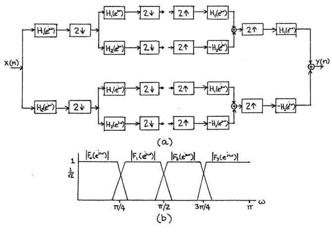
The more straightforward implementation is the tree configuration (Fig. 2-3a). Separation into subbands is done in stages by repeated application of the two-band QMF. The first stage splits the input into a lowpass and a highpass version, which are decimated by two. Each of these signals is then split into two more bands and again decimated. The net effect of the two stages is that of a bank of four integer-band bandpass filters (Fig. 2-3b). Since each of the two-band QMFs at any stage insure aliasing cancellation for their inputs, the cascade of
analysis filters does as well. Thus, a 2t-band QMF can be implemented with t stages of two-band QMFs.
(C)
1
.LL
Cb)
Figure 2-3. Tree Configuration (4-Band)
In Fig. 2-3, the same fundamental lowpass filter, Hl(eJW), is used at each stage (in general this need not be true). It is clear that Hl(ejW) separates lowpass and highpass components in the first stage, but not as obvious is how the same filter can split each of these signals into even narrower bands in the second stage.
As mentioned in Chapter 1, the decimation of an integer-band signal implicitly performs a modulation to the baseband along with a normalization of the frequency axis. This allows the use of H(eJW) in the second stage. Fig. 2-4 illustrates this point. The subsampling
step (multiplying by an impulse train) achieves modulation down to the baseband and throwing out the zero samples normalizes the sampling frequency to the decimated rate. (Roughly speaking, shrinking in the time domain corresponds to stretching in the frequency domain, and vice versa.) Thus, the baseband version of each subband is stretched out so that H(ejw) selects half of it. A consequence of this is that the transition region of filters in the second stage are effectively twice as narrow when considered at the original sampling rate. Therefore, to achieve a specified transition bandwidth for the four net bandpass filters of the QMF analysis, the second stage filters only need about
half as many taps as those in the first stage. For a t-stage QMF, the filters in stage i are typically designed to be half as long as those in stage i-1. This reduces computation costs and delay time.
-iT
rI'
<'1I
* W , TrI
Subsc.mpin9Reiw)
XC '_
I. rN/NI
K/NAn
. . . -IT W o eIThrowrnj ovt ieroQs
-w ,W
7
} Yr'1
. W 'TI
Thnigovtzeoes
K
-TTFigure 2-4. Tree QMF, Frequency Domain (4-Band)
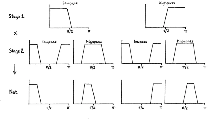
To determine the frequency responses of the 2t composite bandpass filters, we must cascade appropriate filters from each stage while taking into account the differences in sampling rates (Fig. 2-5). Each
S L . -5 - -g -- I I - -- 1I I· -I--- · -! t A) ! ! - 2 S - = i -. . . . - -i %
ifiJ
I.1
net bandpass filter is obtained by choosing a combination of t lowpass or highpass filters, LOoas h;ahoass Stafe i r (owposs iTfz or 1pss Trlz OrI rfz Tr TrjZ v lopass hi VI CS3 . \ I 1 Ir/. . . !r t tr;Z Tr
Figure 2-5. Multiplying Stage Responses
The parallel
QMF (Fig. 2-6) directly
implements the net bank of
bandpass filters,
thereby avoiding the explicit cascading of stages.
The coefficients of the parallel filters
are determined by recognizing
that multiplication of frequency responses is equivalent to convolution of the impulse responses. However, Just as decimation must be considered in the frequency domain, its effects cannot be overlooked in the time domain. In other words, the impulse responses of the ;half-band filters at each stage cannot be directly convolved with one another. To compensate for the different sampling rates, 2i 1-1 zeroes must be inserted between successive taps of the ith stage (upsampling by 2i- 1)
before convolution. It is easy to show that if Mi is the length of the
lowpass or highpass filter of the ith stage of a tree structure, then the impulse response of the corresponding direct parallel implementation has length t L = 1 + (Mi-1)2i - 1 i=1
St
9e 2
Net
(2-10) · =Galand and Nussbaumer have found that the result of this convolution typically contains very small coefficients at the beginning and end of the impulse response [46]. This permits truncation of the impulse response to approximately L = L/t while still achieving adequate aliasing cancellation.
x(n)
-mJ
1
T •F.i h Vuei,
i:H,
J;7L
Figure 2-6. Parallel QMF (4-Band)
Parallel implementations with truncated tap lengths have shorter delays, require less storage, and are less complex than equivalent tree structures while requiring about the same number of multiplications and additions.
2.2.3 Filter Design
In this study a 16-band parallel QMF of length 72 taps is designed by convolving, with decimation adjustment, impulse responses corresponding to lowpass and highpass filters of an associated tree structure.
The first step in designing the filter bank is to come up with a half-band lowpass filter for each of the four stages. Coefficients of the half-band filters were derived using the Remez exchange algorithm for optimal linear phase FIR construction [5]. Filter lengths for stages 1 to 4 were 64, 32, 16, and 10 taps. The actual coefficients are listed in Appendix A. Their frequency responses, as well as those of their mirror image highpass versions, are shown in Fig. 2-7.
1
r1 'LF~rf
r
STAGE
1 -
64
taps
Za -a
M-10
10-20
-30
-50
Z
-60
Z
-70
-80
0
f,/8
fs/4
FREQUENCYSTAGE
2
-
32
taps
*2 inlU
Cr 10z -10
0
Q- -20':
-30
-40
=
-50
Z -60
= -70
-80
3fs/8
f/2
0
f
5
/8
fs/4
3fs/8
fs/2
FREQUENCYSTAGE 3 -
16 taps
fs/8
fs/4
FREQUENCY3fs/8
fs/2
STAGE
4 -
10 taps
0
fs/8
f./4
3fs/8
FREQUENCYfs/2
Figure 2-7.
Half-Band Filters (continued)
/ '-, I ; I
-,,
I 11
Ii I z-.~~~~~~~·- . . - .. / - " III I I,II I~II!
I.i0
20
c
10
W.0
0
z -l0
X
-20
c -30
"
-40
i
-50
Z -60
z
-70
-80
20
M 10 V.W 0 Li.Iz -10
X -20
c -30
L -40~
-50
z -60
: -70
-80
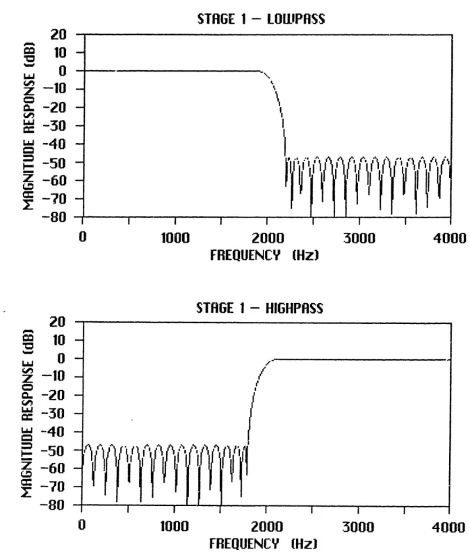
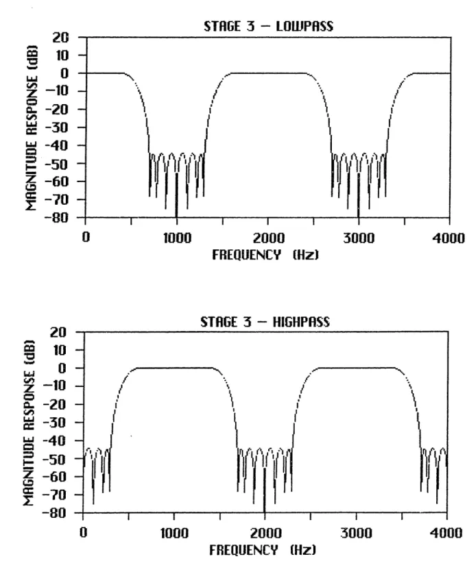
-- __ __~ !v X r ! I I I IAfter normalization to the sampling frequency of stage 1, the frequency responses become
STAGE 1 - LOIPASS
0
1000
2000
3000
FREQUENCY
(Hz)
4000
STAGE 1 - HIGHPRSS0
1000
2000
FREQUENCY I3000
4000
(Hz)
Figure 2-8a.
Normalized Half-Band Filters
(Stage 1)
20
01o
=
10
z-10
X -20
cc -30
-40
I -50z -60
= -70
-80
20
100
z
-10
c
-20
w -30 w-40
-50
Z -60
Z
-70
-80
/~ ~
~ ~~
_II
YVI
I 1' -1 · _ __ I I I lSTAGE
2 -
LOIIIPASS
0
1000
2000
3000
FREQUENCY
(Hz)
STAGE 2 - HIGHPRSS0
1000
2000
3000
FREQUENCY(Hz)
Figure 2-8b. Normalized Half-Band Filters
(Stage 2)
20
Ll10
-1oX
-20
L,=
-30
L
-40
- -50
Z
-60
= -70
-80
20
v
10
10z -10
X
-20
: -30
"
-40
-50
Z
-60
= -70
-80
4000
4000
STAGE 3 - LOWIPASS
0
1000
2000
3000
FREQUENCY (Hz)
STAGE 3 - HIGHPfISS0
1000
2000
3000
FREQUENCY (Hz)Figure 2-8c.
Normalized Half-Band Filters
(Stage 3)
20
10
0
z -10
. -20
w -30
a -40
-50
Z -60
= -70
-80
o
10
LU0
z -10
. -20: -30
-40
.
-50
z -60
: -70-80
4000
4000
STAGE 4 - LOWPASS
\
//
'N
/
11~
~~1
I I I I2000
FREQUENCY t I' I
I
i3000
(Hz)
STAGE 4
-
HIGHPRSS
0
1000
2000
3000
FREQUENCY Hz)Figure 2-8d. Normalized Half-Band Filters
(Stage 4)
0
II000
20
10
LJJ0
z -10
. -20
: -30
-40
z -50
Z -60
:
0 -70
-80
20
2
10
10T-o
. -20
3 -30
w -40-50
Z -60
1. -70-80
4000
4000
__ _ _ - _ _ ___ __ I I I I I IThese filters are convolved to form 16 bandpass filters each of length 258 (see equation (2-10)). The first and last 93 coefficients are truncated to leave 72 taps (see appendix A for coefficient values). The frequency responses of the resulting filters are shown in Fig. 2-9. The composite response of the QMF system, given by
N-1
(2-11) h(n) = fk(n)*gk(n) k=0
where fk(n)xgk(n) is the convolution of the kth bandpass impulse responses of N-band QMF and inverse QMF filter banks, respectively, is plotted in Fig. 2-10.
ONE SUBBAND, F(ejrjL)
6 20 10
z -10
a. -20-30
w -40
-50
z -60
1Z -70
-1
-80
20
10 0z-1o
L-20
= 30
w -40- -50
z -60
= -70
-80
0
1000
2000
3000
FREQUENCY (Hz)PARALLEL BANIPASS FILTERS (16-BAND QMF)
0
1000
2000
3000
FREQUIENCY (liz)
Figure 2-9. 16-Band QMF Bandpass Filters
4000
2.0
M 1.6Z,.
1.2
z 0.8
° 0.4
I" 0.0'i
-0.4
=
-0.8
Z -1.2
= -1.6
-2.0
COMPOSITE RESPONSE, H(eJw)
0
1000
'
2000
3000
FREQUENCY
(Hz)
4000
Figure 2-10. Composite Response, 16-Band QMF
The inherent symmetry of the half-band filters is manifested in certain proper-ties of the parallel filters.
(2-12) fN1-k(n) = (-1)nfk(n) (2-13) gk(n) = N(-1)kfk(n)
These relationships are useful in reducing the amount of computation needed for QF analysis and reconstruction.
2.3 BIT ALLOCATION
The goal of the bit allocation algorithm is to determine the number of bits available for sample encoding (from the specified coder bit rate), and to distribute them among the 13 subbands based upon relative power. Bit allocation is recalculated for every block of 128 input samples (16ms) to dynamically adjust to changes in the input power spectrum.
It is shown in 47] that the total quantization error of a subband coder is minimized with the following bit distribution
N-1 (2-14) n(i) = og2
where ni and Ei are the number of bits and energy, respectively, of the
it h band, 0 < i < N-1. M is the total number of bits available per subband sampling interval.
(2-15)
N-1
M =n i
i=O
This algorithm requires the computation of the energy in each subband. Esteban and Galand suggest a simple alternative [47]. They estimate the energy of a subband during a particular block to be proportional to the square of the maximum sample amplitude.
(2-16) E = a2Ci
i
i
2for some constant a
where Ci = max Isi(j)Ij=l,p
C , the so-called subband characteristic, is the largest value in the i h subband's current block of p samples. Substituting this into (2-14) gives
N-1
(2-17) n(i) = - 1 log2C,
+
+ lo.C2
i j=0
2.3.1 Adjustment Algorithm
In this paper, n(i) is restricted to the range 0 < n(i) < 5 as recommended in [48] and [49]. However, equation (2-17) does not always produce integer values in the desired range. Fig. 2-11 illustrates such a case. Clearly, an adjustment algorithm is needed to determine actual bit allocation based upon the n(i) values.
r,(i) 5 4 3 2 1