CONJOINT PROBABILISTIC SUBBAND MODELING
by
Ashok Chhabedia Popat
S.B. Electrical Engineering, Massachusetts Institute of Technology, 1986
S.M. Electrical Engineering, Massachusetts Institute of Technology, 1990
Submitted to the Program in Media Arts and Sciences,
School of Architecture and Planning,
in partial fulfillment of the requirements for the degree of
Doctor of Philosophy
at the
MASSACHUSETTS INSTITUTE OF TECHNOLOGY
September 1997
@
1997 Massachusetts Institute of Technology
All rights reserved
Signature of Author:
Program in Media Arts and Sciences
August 8, 1997
Certified by:
Rosalind W. Picard
NEC Career Development Pro
sor of Computers and Communications
Tesis Supervisor
Accepted by:
!
--
,,
V A -L
Stephen A. Benton
Chair, Departmental Committee on Graduate Students
Program in Media Arts and Sciences
OK
C)Conjoint Probabilistic Subband Modeling
by
Ashok Chhabedia Popat
Submitted to the Program in Media Arts and Sciences,
School of Architecture and Planning,
on August 8, 1997, in partial fulfillment of the
requirements for the degree of
Doctor of Philosophy
Abstract
A new approach to high-order-conditional probability density estimation is developed,
based on a partitioning of conditioning space via decision trees. The technique is applied
to image compression, image restoration, and texture synthesis, and the results compared
with those obtained by standard mixture density and linear regression models. By
apply-ing the technique to subband-domain processapply-ing, some evidence is provided to support the
following statement: the appropriate tradeoff between spatial and spectral localization in
linear preprocessing shifts towards greater spatial localization when subbands are processed
in a way that exploits interdependence.
Thesis Supervisor: Rosalind W. Picard
Doctoral Dissertation Committee
Thesis Supervisor
-Rosalind W. Picard NEC Career Development Professor of Computers and Communications Program in Media Arts and Sciences
AA
Thesis Reader
Robert .f Gray Professor and Vice Chair Department of Electrical Engineering Stanford University
Thesis Reader
r
Josef Kittler Professor of Machine Intelligence Director of the Center for Vision, Speech, and Signal Processing University of Surrey
Thesis Reader \
Alex Pentland Academic Head and Toshiba Professor of Media Arts and Sciences Program in Media Arts and Sciences
ACKNOWLEDGMENTS
I would like to thank Professor Rosalind Picard for her advice, encouragement, support, and patience over the years. She has made an effort to make working in her group enjoyable, and has taught me a great deal along the way.
I would also like to thank the other members of my committee: Professors Robert Gray, Josef Kittler, and Alex Pentland. Professor Gray provided needed guidance and encouragement at several stages of this work. Some of his early comments in a discussion we had in Adelaide in early 1994 picqued my interest in the use of decision trees for density estimation. Both Professor Gray and Professor Kittler traveled great distances to attend my defense; it was a great pleasure and a privilege for me to have had each of them serve on my committee. Professor Pentland's early work and comments about predicting subbands were inspirational, and every conversation I've had with him has been a pleasure and a learning experience.
Many other people helped me greatly along the way, including most of the Vision and Modeling Group and much of the Garden. It is not possible to list all of them here individually; a partial list follows: Professor Ted Adelson, Dr. Rich Baker, Jeff Bernstein, Professor Aaron Bobick, Sumit Basu, Professor Michael Bove, Bill Butera, Lee Campbell, Dr. Ron Christensen, Thunyachate (Bob) Ekvetchavit, Dr. Bill Freeman, Professor Bernd Girod, Anh Viet Ho, Tony Jebara, Professor Michael Jordan, Professor Murat Kunt, Dr. Wei Li, Professor Jae Lim, Fang Liu, Tom Minka, Professor Bruno Olshausen, Professor Al Oppenheim, Ken Russell, Professor William Schreiber, Professor Eero Simoncelli, Dr. Andy Singer, Professor David Staelin, Thad Starner, Dr. Gary Sullivan, Martin Szummer, Dr. John Y. A. Wang, Yair Weiss, Chris Wren, and Professor Ken Zeger.
Most of all, I'd like to thank my wife Rita for being the best part of my life, and for making me a part of hers.
This research was supported in part by Hewlett-Packard Company and NEC Corporation. Some of the expressions used in the software were obtained using MACSYMA, courtesy of the U.S. Department of Energy.
CONTENTS
CH A PTER 1: Introduction ... 10
1.1 Conjoint Processing ... ... ... 11
1.2 Independence in Im age Subbands ... ... 12
CH A PTER 2: Background ... . ... 14
2.1 Subband-Dom ain Processing ... 14
2.2 D ensity Estim ation ... 19
2.3 Evaluation Criteria for Density Estimation ... 31
2.4 Histogram, Kernel, and Mixture Density Models ... 39
2.5 Mixture Estimation via the Generalized Lloyd Algorithm ... ... 44
2.6 Mixture Refinement via Expectation-Maximization ... 46
2.7 Conditional Density Estimation using Finite Mixtures ... 49
2.8 C hapter Sum m ary ... 55
CHAPTER 3: Partitioned Conditioning via Decision Trees ... 56
3.1 Trees: Basic Concepts, Notation, and Terminology ... ... 56
3.2 Tree-Induced Partitions and the Hard PCDT Model ... 57
3.3 G row ing the Initial Tree ... 58
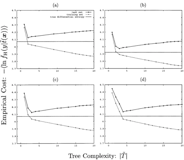
3.4 Determination of Appropriate Tree Complexity (Pruning) ... 61
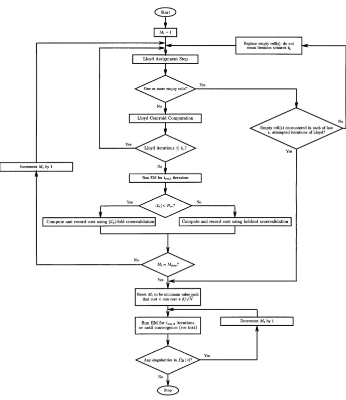
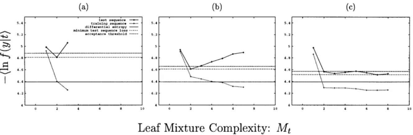
3.5 F itting the Leaves ... 66
3.6 Variations on PCDT: Softening the Splits and Hybrid Modeling ... ... 71
3.7 Implementation Considerations ... 72
3.8 M ore E xam ples ... 72
3.9 Discussion of New Work Relative to Prior Work ... 75
3.10 C hapter Sum m ary ... 79
CHAPTER 4: Conjoint Image and Texture Processing ... 81
4.1 Lossless Compression of Greyscale Images ... 81
4.2 Conjoint Scalar Quantization ... 84
4.3 Sequential Texture Synthesis ... 91
4.4 M ultiresolution Texture Synthesis ... 92
4.5 Im age R estoration ... 95
4.6 Relationship to other m ethods ... 98
4.7 C hapter Sum m ary ... 99
CH A PTER 5: Preprocessing ... 101
5.1 One-band Subband Coding ... 101
5.2 Filter Banks for Conjoint Subband Coding ... 103
5.3 Conjoint Subband Texture Synthesis ... 108
5.4 C hapter Sum m ary ... 110
CHAPTER 6: Recommendations for Further Work ... ... 111
6.1 PCDT ... ... 111
6.2 Applications ... ... 113
6.3 Subband C oding ... 114
C H A P TER 7: C onclusions ... 115
APPENDIX A: Economized EM Algorithm for Mixture Estimation ... 118
APPENDIX B: Variable-Localization Filter Banks ... 122
LIST OF FIGURES Figure 1.2.1: Figure 2.1.1: Figure 2.1.2: Figure 2.1.3: Figure 2.4.1: Figure 2.4.2: Figure 2.7.4: Figure 2.7.5: Figure 3.4.1: Figure 3.4.4: Figure 3.5.1: Figure 3.5.2: Figure 3.8.2: Figure 3.8.3: Figure 4.1.1: Figure 4.1.2: Figure 4.1.3: Figure 4.2.1: Figure 4.2.2: Figure 4.2.5: Figure 4.4.1: Figure 4.4.2: Figure 4.4.3: Figure 4.5.1: Figure 4.5.2: Figure 5.1.1: Figure 5.1.2: Figure 5.2.1: Figure 5.2.2:
Natural Image Decomposed into 3 x 3 Subbands...12
Critically Sam pled Filter Bank ... 15
Three-Level Subband Pyramid ... 16
Spectral-Domain Illustration of Within-Subband Uncorrelatedness ... 16
Two-Pixel Neighborhood for Vector Extraction ... ... 40
Example Comparing Histogram, Kernel, and Mixture Density Estimates ... 41
Joint versus Conditional Mixture Optimization ... 50
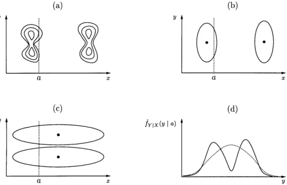
Example distribution for which PCDT outperforms EM ... 54
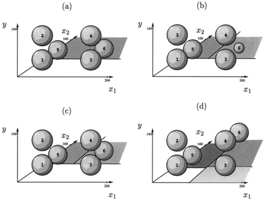
Example Mixtures Leading to Different Tree Configurations ... 63
Empirical PCDT Splitting/Pruning Cost versus Tree Complexity ... 64
Flow Chart of Leaf-Mixture Complexity Determination and Fitting ... 67
Empirical Leaf-Specific PCDT Cost versus Mixture Complexity ... 69
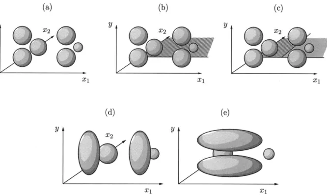
Gaussian Density Exhibiting Both Irrelevance and Linear Dependence ... 73
Example of the Performance/Complexity Tradeoff for EM and PCDT ... 74
Arithm etic Coding of Im ages...82
Semicausal Pixel Neighborhoods... ... 83
The cman and Lenna Test Images...83
Sequential Predictive Entropy-Coded Scalar Quantization System...86
Predictive Coding of a Third-Order Gaussian Autoregressive Process...87
Sequential Texture Synthesis by Sampling from
fyg
... 90Conditioning Neighborhoods for Multiresolution Texture Synthesis ... 92
Multiresolution Sequential Texture Synthesis Examples ... 93
Evolution of Detail in Deterministic Multiresolution Texture Synthesis ... 94
Restoration Neighborhoods... ... ... 96
Example of Conjoint Image Restoration... 96
Robust Quantization System using Time-Dispersive Filtering ... 102
Vector Quantization of a Filtered Gamma Source with Varying Blocklength. 102 Frequency-Magnitude Responses for a Set of Filter Banks ... 105
Figure 5.2.4: Figure 5.2.5: Figure 5.2.6: Figure A.1:
Conjoint and Independent Coding Performance vs. Spatial Dispersiveness.. 106
Critically Sampled Perfect-Reconstruction Filter Bank as a Multiplexer ... 107 Effect of Filter Dispersiveness in Subband Texture Synthesis ... 108 Typical Computational Savings Achieved by Economized EM Algorithm.... 119
LIST OF TABLES
Table 3.4.2: Parameters for Mixture Density Shown in Figure 3.4.1(a) ... 63
Table 3.4.3: Parameter Differences from Table 3.4.2 for Figures 3.4.1(b-d) ... 63
Table 3.5.3: Number of Possible Leaf Complexity Allocations...70
Table 3.8.1: Example Performance of PCDT vs EM...73
Table 4.1.4: Lossless Compression Rates (bpp) for the cman Image ... 84
Table 4.2.4: Lossy Compression Rates (bpp) for the cman Image ... ... 89
Table 5.2.3: Spatial Dispersiveness of Filters Shown in Figures 5.2.1 and 5.2.2 ... 105
CHAPTER 1:
Introduction
Generally, there is a theoretical performance advantage in processing data jointly instead of sepa-rately. In data compression, for example, the advantage of joint processing results from the ability to exploit dependence among the data, the ability to adapt to the distribution of the data, and the ability to fill space efficiently with representative points [45, 71].
It is generally much easier and often more natural to process data sequentially than jointly. It is of interest, therefore, to find ways of making the performance of sequential processing approach that of joint processing to the extent possible. There are some situations in which sequential processing does not incur a large performance penalty, for instance when compressing independent data. This case is of limited interest however, as real information sources are seldom usefully modeled as independent. A more interesting example is compression of data that is not required to be independent. In lossless compression, a message is to be represented in compact form with no loss of information. It is well known that the best lossless encoding will produce on average a number of bits about equal to the minus log of the joint probability that has been assigned to the message [124]. However, it is difficult to work with the set of all messages, even if we restrict consideration to those of a fixed moderate length. By simply writing the joint probability as a product of conditional probabilities of the individual letters, we can achieve the same compaction sequentially by using the optimum number of bits for each letter. The order in which we encode the letters can be arbitrary, though often a natural ordering is suggested by the application.
The key to effective sequential lossless data compression lies in finding the right conditional probabilities to use. This generally requires that some structure or model be assumed, and that the probabilities be estimated from the data with respect to that model. Thus, the problem of lossless compression is really one of modeling the sequence of conditional probability distributions.
It is natural to seek to generalize this strategy to applications besides lossless data compres-sion, hopefully in a way that likewise approximates the performance of joint processing. This thesis proposes that the generalization be accomplished through the use of high-order conditional probabilistic modeling.
1.1 Conjoint Processing
We use the term conjoint processing to refer to the sequential processing of data according to a corresponding sequence of conditional probability laws chosen such that their product approxi-mates the joint probability law. This approach to processing information has been advocated by Rissanen [108, 1111. Our choice of term is somewhat arbitrary, but it is convenient to have a short way of describing this style of processing. The dictionary definition of "conjoint" is not much different from that of "joint;" both can be taken in our context to mean roughly "taking the other values into account." Since "joint" is already claimed, we instead appropriate the term "conjoint" for our purpose. A related term coined by Dawid [30] is prequential (for predictive sequential), but it has come to be used in a relatively narrow statistical sense, rather than to describe a general style of processing information.
There are many areas in which conjoint processing is currently being employed, though not always to the full potential afforded by its framework. We have already considered lossless com-pression. What would be required to extend the technique effectively to lossy compression, where the message need not be reconstructed perfectly? In most applications of interest, we would need to be able to model and estimate conditional probability laws accurately when the data are con-tinuous or well approximated as concon-tinuous. If the lossless case is any indication, the accuracy of such modeling will have great impact on the performance achieved by a conjoint lossy compressor. To begin to take full advantage of the conjoint processing framework then in a general setting, we must be able to model conditional densities accurately.
This thesis proposes a technique for accurately modeling conditional densities (Chapter 3). The technique combines aspects of decision trees and mixture densities to achieve accurate modeling by appropriately partitioning conditioning space, while exploiting the known smoothness of the underlying probability law. An important feature is that it adjusts its complexity automatically to an appropriate level for the data, avoiding overfitting while still allowing sufficient flexibility to model the data effectively.
Conjoint processing can be used successfully in applications other than data compression. This is shown in Chapter 4, where it is applied to texture synthesis and image restoration in addition to compression. In the texture synthesis application, it is found that conjoint processing can result in synthesized textures that have characteristics more realistic than those obtained using standard
Horizontal band 1
Vertical band 0
Vertical band 1
Vertical band 2
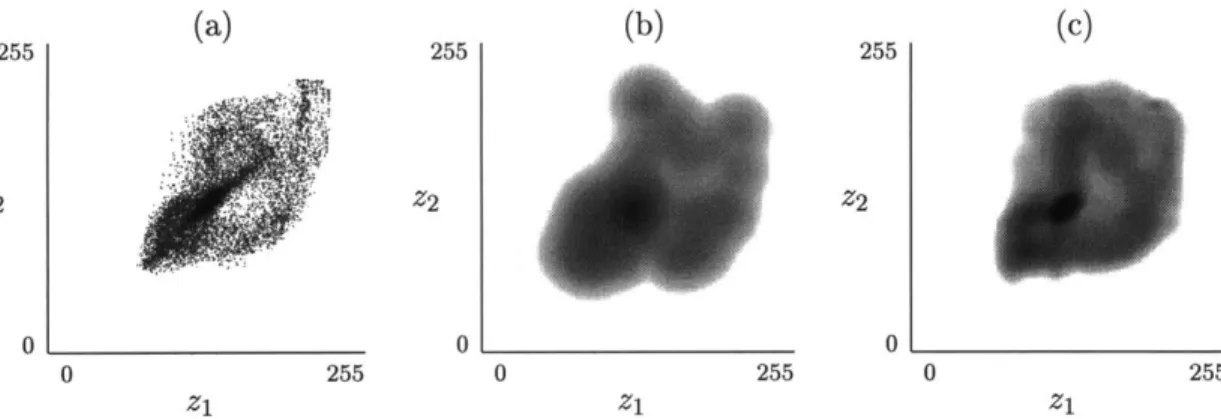
Figure 1.2.1: Separable 3 x 3 uniform-band subband decomposition of the luminance component of the standard 720 x 576 test image Barbara. A jointly localizing, quasi-perfect-reconstruction, critically sampled analysis filter bank designed using the method described in [92] was used. The non-DC bands have been shifted and scaled in amplitude for display. Strong spatial and spectral interdependence of subband pixels is evident, yet the empirical correlation is nearly zero among pairs of non-DC pixels for a variety of displacements, both within and across subbands. It may be concluded that there is a great deal of nonlinear dependence.
techniques. It is also shown to perform effectively in image restoration because of its ability to model nonlinear relationships over relatively broad spatial areas.
1.2 Independence in Image Subbands
In subband coding, an image is broken up into several frequency bands called subbands, after which each is subsampled spatially. The subsampled subbands are then lossy-compressed as if they were independent - that is, by using techniques which are known to work well under the assumption that the data are independent. After decoding, the reconstructed subbands are pieced back together to form an approximation to the original image. Subband coding will be described more fully in Section 2.1, and an explanation will be given there for why the subband pixels are usually modeled as approximately independent, or more precisely, uncorrelated.
12
In practice, pixels in subbands formed from an image of a natural scene are far from indepen-dent. An example is shown in Figure 1.2.1. Recently, there has been growing interest in extending the traditional subband coding approach to take advantage of this dependence. One approach is to group subband pixels into disjoint sets and to quantize the pixels in each set jointly, ignoring any interdependence between sets. This approach to subband coding is an active area of research; see the recent paper by Cosman et al. [25] for an extensive survey. Also described there are techniques that we might call conjoint, except that, as far as I am aware, the conditional distribution is either modeled only implicitly as in [126], or explicitly but using fairly restrictive models as in [73]. It would be interesting to see whether an explicit, powerful conditional density model such as that described in Chapter 3 might be used advantageously in such systems. This question is considered in Chapter 5.
The purpose of the subband decomposition, which is clear when independent compression of the subbands pixels is employed (see Section 2.1), is less clear when joint or conjoint compres-sion is allowed. The question of what filter characteristics are best to use in this case must be answered on the basis of practical rather than theoretical considerations. This is because most subband decompositions that one would normally consider for use today are reversible or nearly so, implying that all are equally good (or in this case, equally without effect) when unconstrained joint compression is allowed. When restrictions are placed on the complexity and dimensionality of the processing, as they must be in practice, the problem becomes one of joint optimization of the subband decomposition and the characteristics of the subsequent processing. Such an opti-mization can be feasible if the system is sufficiently constrained; for example, Brahmanandam et al. [11] have considered jointly optimizing an affine block transform and a vector quantizer. A more general optimization procedure for a fixed encoding scheme might be to select a structure for the subband decomposition, then search over filters to use in that structure that achieve varying levels of tradeoff between spatial and spectral localization. Such a search is also considered in Chapter 5. Evidence is presented there to support the conjecture that in some applications, preprocessing filters that achieve greater spatial localization are required when joint or conjoint processing is used than are required when independent processing is used.
CHAPTER 2:
Background
This chapter provides background information relevant to subband-domain processing and density estimation.
2.1 Subband-Domain Processing
Subband-domain processing is a generic term given to a family of procedures that operate by
divid-ing the frequency spectrum into approximately disjoint regions called subbands, processdivid-ing each, and combining the results to get a desired output. The division into subbands is called analysis and the recombination is called synthesis. A good general reference on the subject is the textbook by Vetterli and Kovacevic [138]. We shall briefly summarize the essentials, explain why subband pixels tend to be approximately uncorrelated, and summarize how subband decompositions have traditionally been used in image compression.
Critically Sampled Filter Banks
The basic building-block in analysis and synthesis is the critically sampled filter bank, a special case of which is shown in Figure 2.1.1. It is a special case because in general the subsampling factors need not be equal; however, the sum of their reciprocals must equal unity if they are to be critically sampled. Critical sampling refers to retaining the minimum number of samples necessary to reconstruct the filter outputs under the assumption that the filters are perfectly frequency-selective. If the output is equal to the input in the event of no intermediate corruption of the subbands, then the filter bank is said to have the perfect-reconstruction property. The filters need not be perfectly frequency-selective in order for the perfect-reconstruction property to hold. Henceforth, all of the filter banks considered will be assumed to have the perfect-reconstruction property.
The subsampling operations indicated by the blocks labeled
4
K involve discarding all samples except every Kth one. To describe this operation precisely, it is necessary to specify a subsampling phase, which indicates the offset of the retained sample indices relative to the multiples of K. The upsampling operations denoted byt
K replace the retained samples into their original sequenceAnalysis Synthesis
P-H,(z)
LITE
, z
Input -H2(z) G2 (z) + --- Output
HK(z)
LoK
GK(Z)
Figure 2.1.1: A critically sampled filter bank, consisting of an analysis and a synthesis stage.
The system shown is for processing a one-dimensional signal; it may be applied to images by applying it in the horizontal and vertical directions separately.
phases can be and often are different for every band. A trivial perfect-reconstruction critically sampled filter bank can be obtained by taking every filter to be an identity operation and the subsampling phases to be a permutation of (0,... , K - 1). Henceforth, subband will refer to the filtered signal after subsampling.
The foregoing description assumes one-dimensional signals. The structure can be extended to two or more dimensions in a general way. A simpler alternative, which is standard practice in image subband coding, is to perform two-dimensional subband analysis and synthesis by performing the one-dimensional operations separately in the horizontal and vertical directions. Two-dimensional critically sampled filter banks that can be implemented in this way are termed separable. Consid-eration will be restricted to separable critically sampled filter banks throughout this thesis.
Often, an unequal division of the frequency spectrum is desired. One can be obtained by using a more general filter bank with an appropriate choice of filters and subsampling factors. However, here we restrict consideration to uniform-bandwidth critically sampled filter banks. Using these, an unequal spectral division can be obtained by recursively performing subband analysis on selected subbands, resulting in a tree-structured decomposition. Often, only the lowest-frequency subband is recursively subdivided. In this case, when the analysis is carried out separably in the vertical and horizontal dimensions, the decomposition is termed a subband pyramid, or
just
apyramid (see Figure 2.1.2). Such a structure can also be used to implement certain discrete wavelet
transforms [138]. We will restrict consideration to pyramids obtained by using the same two-band critically sampled filter bank to carry out all of the analyses. Moreover, the filter banks considered will be orthogonal in the sense defined by Simoncelli and Adelson [131).
Horizontal Frequency
Figure 2.1.2: Construction of a three-level subband pyramid. An image is analyzed into four subbands as shown in (a) by applying a two-band critically sampled filter bank separately in the horizontal and vertical directions. These four subbands constitute the first level of the pyramid. The analysis is then repeated on the low-horizontal, low-vertical frequency subband, resulting in the two-level pyramidal decomposition shown in (b). Repeating the analysis once more on the new low-horizontal, low-vertical frequency subband results in the three-level pyramidal decomposition shown in (c). Because all of the subbands are critically sampled, the total number of pixels in the pyramidal representation is equal to that in the original image.
4n ii L t L 4 24 L 4 L L a 2: 2
Figure 2.1.3: A spectral-domain illustration of within-subband uncorrelatedness. A hypothetical
signal having the lowpass magnitude spectrum shown in (a) is input to an ideal four-band critically sampled filter bank. The spectrum of the output of H2(z) before subsampling is shown in (b), while that after subsampling (scaled in amplitude by a factor of four) is shown in (c). Note that after subsampling, the spectrum is relatively flat, implying that pixels within a given subband are approximately uncorrelated. Assuming a smooth input spectrum, flatness increases as the filters get narrower, which in a uniform filter bank corresponds to increasing the number of bands. For natural images, the assumption of smooth spectrum is grossly violated in the lowest-frequency
(DC) band, so that the DC band in general cannot usefully be modeled as uncorrelated.
Uncorrelatedness of Subband Pixels
An important property of subband representations is that subband pixels for natural images tend to be approximately uncorrelated, both within and across subbands. Uncorrelatedness across sub-bands can be understood by viewing the subband decomposition as a generalization of an energy-compacting orthogonal block transform, where the basis vectors are allowed to extend beyond the block boundaries. For an orthogonal block transform, diagonalization of the covariance matrix oc-curs as a by-product of maximizing energy compaction subject to the constraint of constant total energy [62]. Therefore, to the extent that an orthogonal subband decomposition achieves energy
compaction, pixels are uncorrelated across subbands.
4 4
Approximate uncorrelatedness within subbands can be easily understood in the frequency domain. The spectra of natural images are often modeled as smooth, except at near zero-frequency (DC) where there tends to be a strong peak. Assume that the analysis filters have nearly ideal narrow brickwall frequency responses. Then for any subband except the one containing DC, the spectrum of the output of the analysis filter will be approximately flat within the passband and zero outside the passband, as shown in Figure 2.1.3 (b). To show that the correlation of pixels in the subband is nearly zero, it is sufficient to show that after subsampling, the magnitude spectrum is nearly flat across the whole spectrum [84]. Let u[n] denote the output of the analysis filter and let v[m] denote the result of subsampling u[n] by a factor of K, so that
v[m] = u[Km].
For simplicity, a subsampling phase of zero has been assumed; a nonzero subsampling phase would result in an identical magnitude spectrum. By using the fact [114] that
K-1
- K if n 0(modK);
k=0 e
0 otherwise,
we can express the z-transform of v[m] in terms of that of u[n] asIK-1 27k1K)
V(z) =
(
U(e-ikz1|Kk=0
which corresponds to a discrete-time Fourier transform of
1 K-1
V(w) = K
U([w
-
27rk]/K).
k=0
In this way, the filter passband is mapped onto the entire spectrum [-7r, 7r], which under the stated assumptions results in an approximately flat spectrum as indicated in Figure 2.1.3 (c). Thus, pixels within the subbands are approximately uncorrelated.
The approximate uncorrelatedness within and across subbands does not imply approximate independence of the subband pixels, as previously noted in Chapter 1.
Subband coding of images
Subband and subband-pyramid decomposition are often used in lossy compression. Subband-based lossy compression is termed subband coding. Subband coding was first applied to speech [62] in the seventies and extended to images in the mid-eighties [143]. Much of the underlying motivation and
theory carries over directly from an older technique called transform coding [56]. As mentioned above, a block transform is a special case of subband decomposition. The basic idea behind image subband coding is now reviewed briefly.
The analysis of an image into subbands by a critically sampled filter bank results in an exact representation of that image with no reduction in the total number of pixels. Although no com-pression occurs in the decomposition, it is an empirical fact that for natural images the subbands tend to be easier to compress than the original image. In particular, a subband decomposition generally results in a predictably uneven distribution of energy among the subband pixels, so that the available code bits can be allocated among the subband pixels in accordance with how much they are needed. In addition, the subband pixels are nearly uncorrelated as discussed above, so that they can be quantized independently using scalar quantization with reasonable efficiency.
Typically, subband pixels are modeled as having a variance that changes slowly over space and spatial frequency. Suppose that the subband pixels have been grouped into subsets, each characterized by a local variance o?. The pixels in each subset are typically taken to be nearby one another in both space and spatial frequency. Assuming independent scalar quantization, high rate, small quantization bins, and smooth densities, the mean-square per-pixel quantization error for each subset can be approximated as Eo?2- 2Ri , where Ri is the average rate allocated to subset
i and c is a performance factor which depends on both the type of quantizer and on the marginal
distribution of the pixels [62]. If the variances are large enough so that no negative rate allocations would result, then the method of Lagrange multipliers can be used to derive the asymptotically (high rate) optimal rate allocation
1
RR + -log 2 of (2.1.4)
2
where RO is a constant selected to meet the constraint on the total available rate. In this case, the improvement in mean-square error (MSE) over quantizing the original pixels can be approximated by the ratio of the arithmetic to the geometric mean of the variances [62]. Neither (2.1.4) nor this formula for the improvement is valid in the important case where one of more of the variances are nearly zero, as this would result in negative rate allocations which would violate the assumption behind the use of Lagrange multipliers. In such situations, an optimal iterative rate allocation procedure can be used instead [58, 127], but a simple formula for the improvement in MSE no longer exists in general.
Alternatively, rate can be allocated implicitly by entropy-coded uniform-threshold scalar quan-tization (see Section 2.3). In this case the rate allocated to each subband is determined by the activity of the subband pixels and by the stepsize of the quantizer. Using the same stepsize for all subband pixels can be shown to result in a nearly optimal implicit rate allocation with respect to mean-square error [42, 93]. A frequency-weighted mean-square error criterion can be easily accom-modated by varying the stepsizes across subbands, as is implicitly done in JPEG [101]. Perceptually optimized rate allocation has been considered by Jayant et al. [61] and Wu and Gersho [144].
As mentioned previously, subband pixels exhibit a great deal of statistical dependence de-spite their near-uncorrelatedness. This dependence may be exploited for coding gain in a number of ways [25]. In Chapter 5, we will consider exploiting the dependence by conjoint processing; specifically, by sequential scalar quantization with conditional entropy coding.
2.2 Density Estimation
This section introduces ideas and notation related to probabilistic modeling in general and to density estimation in particular.
Heuristic Introduction
In general terms, the problem of density estimation is to infer the probability law hypothesized to govern a random object on the basis of a finite sample of outcomes of that random object as well as on any available prior information. The term "random object" will be defined later in this section. Density estimation is an example of a problem in inductive inference, and inherits all of the well-known foundational difficulties attendant to that class of problem [23, 105, 136, 139]. In particular, induction is not deduction: it is not possible on the basis of observing a finite sample to show analytically that a particular density estimate is correct or even reasonable, unless strong assumptions are made that reach beyond the information present in the available data. The following thought experiment, presented with a sampling of the more popular ways of approaching it, will help to clarify this point.
Imagine being presented with a large opaque box, perhaps the size of a refrigerator, and told that it contains a large number of marbles of various colors. You reach your hand in and pull out ten marbles, one at a time (but without replacement). Suppose that the first nine are red and the tenth is blue. Based on this sequence of observations, you wish to infer the proportion of every color represented among the remaining marbles in the box. This is essentially the density
estimation problem in the discrete case. (A continuous version, discussed later in this section, might involve the weights of the marbles instead of the colors.)
A starting point would be to assume that the order in which the marbles are observed is irrele-vant. This assumption of independence (or exchangeability in Bayesian parlance [43]) is reasonable if the box had been shaken before you reached in, and if the number of marbles in it is in fact very large. Relaxing this assumption will be considered later.
At this point there are several ways in which you might proceed, and none can be shown analytically to be superior to another without making additional assumptions about the contents of the box. Fisher's celebrated maximum likelihood (ML) principle gives the proportions as 9/10 for red, 1/10 for blue, and zero for any other color. To be useful in practice, this principle must usually be modified; often this is accomplished by adding a penalty term [129, 130]. Laplace's rule of succession [85] requires that you know the possible colors beforehand; if there are (say) five of them, then his rule results in the estimated proportions 2/3 for red, 2/15 for blue, and 1/15 for each of the three remaining unseen colors. The minimum-description length (MDL) principle chooses the proportions that result in the shortest possible exact coded representation of the observed data, using an agreed upon prefix-free code for the empirical distribution itself [3, 109]. See [137], p. 106 for an interesting criticism of this approach. In this particular example, again assuming five possible colors, Laplace's rule and MDL happen to agree on the estimated proportions when the prior probability of each empirical distribution is taken to be proportional to the number of possible sequences of marbles that support that distribution;1 that is,
10!
P (Nred, Nblue 510 (Nred)!(Nblue)! ...
where the N's are constrained to be integers between 0 and 10 inclusively. (It is easiest to demon-strate that Laplace's rule and MDL give the same result in this case by computer simulation; the optimized description length turns out to be about 20.6 bits.) Both in this case and typically, the MDL principle functions by initially "lying" about the empirical proportions, then subsequently correcting the lie when the observed sequence of ten marbles is specified exactly using an ideal (with respect to the lie) Shannon code. This particular version of MDL assumes a simple two-part model/message lossless encoding of the observed data, and corresponds to Rissanen's earliest work on MDL [106]. His subsequent work generalizes the MDL principle considerably, removing the strict model/data separation, and allowing variable precision representation of the model
param-1 In other words, proportional to the cardinality of the type class [26].
eters [110]. It should be emphasized that the immediate goal of the MDL principle is inference, not data compression: the hope is that the lie turns out to be a more accurate description of the remaining contents of the box than the truth.
Another point of view is the Bayesian; it is quite different in its motivation from those men-tioned above, and involves the following sort of reasoning. You believe that the box was carried up from the basement, where you know you had stored two boxes: one containing an equal number of red and blue marbles, and the other containing only red. Since a blue marble was among those observed, you reason that the proportions must be 1/2 red and 1/2 blue. In a more fully Bayesian setting, the two boxes would have possibly unequal chances of being picked, but this is a minor point. The main Bayesian leap (from Fisher's point of view, not Rissanen's) is to view the propor-tions themselves (or more generally, anything that isn't known with certainty) as being described by a probability distribution. Rissanen uses a prefix-free code, which amounts to the same thing via the Kraft inequality [41].
It is even possible to argue coherently for estimating a lower proportion of red than blue. A rule that does so is termed counterinductive [136]. One way to justify such an estimate would be on Bayesian grounds, using a suitable prior. Another justification, valid in the case of a small total marble population, would be on the grounds that more red marbles than blue have been used up by the observation sequence. Misapplying this reasoning to the case where the sampling is done with replacement, or where the population is infinite, leads to the well known gamblers' fallacy of betting on an infrequently observed event because "it is due to occur."
The main reason for presenting the foregoing brief survey of the differing major views is to emphasize that there really is no generally agreed upon best way to perform density estimation, and also to underscore the crucial role played by assumptions and prior information.
Assumptions become even more important in the continuous case. Suppose now that the distribution of the weights of the marbles, rather than their colors, is in question, and that all of the ten marbles drawn differ in weight slightly. The added difficulty now is that there is no natural a priori grouping of events into like occurrences; instead, one must be assumed. Usually, this is done implicitly in the form of a statement like, "if one-ounce marbles are frequent, then marbles weighing close to an ounce must also be frequent." A statement of this type amounts to a smoothness assumption on the density, with respect to an adopted distance measure in the observation space.
So far in this example, we have considered only a single characteristic of the marbles at a time; that is, we have considered only scalar density estimation. An example of multivariate or joint density estimation would be when not only the weight of the marbles, but also their size and perhaps other characteristics, are brought into question. These characteristics may of course interact, so that each combination of characteristics must be treated as a different occurrence (unless and until it is found out otherwise). The added complication here is quantitative rather than qualitative: as the number of characteristics or dimensions grows, the number of possible combinations grows exponentially, as does the requisite number of observations required to obtain a reliable density estimate. In the continuous case, it is the volume of space that grows exponentially rather than the number of possible combinations, but the effect is the same. The general term used to refer to difficulties ensuing from this exponential growth is the curse of dimensionality (see [120], pp. 196-206 for a good discussion).
A similar problem plagues conditional density estimation, which refers to the estimation of proportions within a subpopulation satisfying a specified condition. An example would be esti-mating the proportion of marbles that are about an inch in diameter among the shiny ones that weigh about an ounce. Since the number of possible conditioning classes grows exponentially in the number of characteristics conditioned on, exponentially more observations are likely to be required before a reliable conditional estimate can be obtained.
A final complication arises when the order in which the marbles are observed is considered to be significant; that is, when successive observations are regarded as dependent. In such cases, it is natural to view the sequence of observations as constituting a sample path of a random process [48, 84]. In this framework, the marbles are assumed always to come out of a given box in the same fixed sequence, but the box itself is assumed to have been selected at random from a possibly infinite collection or ensemble of boxes, according to some probability distribution. This is not the same as the Bayesian point of view described above, since in this case there is only one level of randomness. Since only a single box is observed, it is necessary that certain assumptions be made so that the observations over the observed sequence can be related to statistics across boxes. The chain of inference must proceed from the specific observed initial subsequence, to the ensemble statistics across boxes for the subsequence, to the ensemble statistics for the whole sequence, and finally to the statistics of the remainder of the sequence in the particular box at hand. To enable such a chain of inference, strong assumptions must be made about the random process. At the very least, it must be assumed that the relevant statistics across boxes can be learned by looking at the contents of
only a single box; roughly speaking, this is to assume that the process has the ergodic property [45]. In addition, in practice some sort of assumption regarding stationarity (invariance of statistics to shifts in time) and the allowed type of interdependence among observations must be conceded. Many specialized processes, each defined by its own set of assumptions, have been proposed over the years; of these, the most useful have been ones in which dependence is limited and localized. The simplest is the stationary Markov process of order m, in which the conditional density of each observation given the infinite past is stipulated to equal that given the past m observations, and, moreover, this conditional density is assumed unchanging over the entire sequence. Such a model is readily generalized to two-dimensional sequences by the notion of Markov random
field, which has been used extensively in texture and image processing [60]. Relaxation of strict
stationarity can be introduced in a controlled and extremely useful manner via the concept of the
hidden Markov source [102] and its various generalizations, which have found application in speech
processing, gesture recognition, and other important areas. Interestingly, hidden Markov models were discussed in the context of source coding by Gallager [41, Chapter 3] more than a decade before they became popular in speech processing.
For the remainder of this chapter, successive observations will be assumed to be independent. This is not as restrictive as it may sound, because the observations will be allowed to be multivari-ate and high-dimensional. In particular, the estimation of high-order conditional densities will be considered extensively. High-order conditional densities are those in which many conditioning vari-ables are used. In the applications to be considered in subsequent chapters, the conditioning orders range between zero and fourteen. Conditional densities can be used to characterize a stationary mth-order Markov process by simply sliding a window of length m +1 along the observed sequence, and, at each position, taking the observations that fall within the window as the observed vector. Subsequent chapters will employ this device often, extending it as necessary to multidimensional sequences (e.g., image subbands).
Basic Terms and Notation
Since the topic at hand is probability density estimation, it seems appropriate to begin the techni-cal discussion by briefly reviewing relevant terms and concepts from elementary probability theory. Besides making the presentation more self-contained, such a review offers the opportunity to in-troduce notation in a natural way, and will also allow us to develop a slightly simpler, albeit more restrictive, notion of density than is usually presented in textbooks.
A rigorous, measure-theoretic approach will not be taken here, for three reasons. First, the density estimation techniques to be discussed involve complex, data-driven procedures such as tree-growing and -pruning, for which a theoretical analysis would be difficult, though considerable progress has been made in this general area - see the recent work by Lugosi and Nobel [74], Nobel [81), Nobel and Olshen [82] and Devroye et al. [34, Chapters 20-23]. Second, the techniques and analyses to be presented were arrived at through practically motivated, somewhat heuristic reasoning, and it is desirable from a pedagogical standpoint not to obscure this path through
post hoc theorizing. Finally, the added precision afforded by a formal approach would have bearing
mostly on asymptotic analysis, whereas in practice near-asymptotic performance is seldom reached, especially in the high dimensional setting. Although some theoretical analysis is in fact possible in the case of finite samples, the resulting conclusions would necessarily be given in terms of a probability measure which, in practice, remains at all times unknown.2 In other words, a precise and rigorous theoretical analysis would ultimately require that the true distribution be known, either explicitly, or else implicitly as contained in an infinitely large sample.
Proceeding informally then, we begin by defining a random object to be an experiment which produces, upon each performance or trial, a result called an outcome. The random object is hypothesized to be governed by a fixed probability law which specifies, for any set A of interest, the probability Prob[A] that the outcome will lie in A on any trial. It is assumed that Prob[] satisfies the usual requirements of a probability measure: nonnegativity, normalization, and countable additivity [2]. The quantity Prob[A] can be interpreted as (but need not be defined in terms of) the limiting relative frequency of values that lie in A in a hypothetical, infinitely long sequence of trials.3
A random variable is a random object having scalar-valued outcomes, and a random vector is a random object having vector-valued outcomes. It will be assumed throughout that all vector
2 Such assumptions can be self-serving, as Rissanen points out in Chapter 2 of [110]. For
instance, if a lossless source code produces 5000 bits in encoding a particular sequence of 1000 binary outcomes, then it should come as little consolation when the designer of the code claims
(even if correctly) that the expected code length is only 200 bits.
3 Although there is now nearly universal agreement about what the axioms in a mathematical theory of probability ought to be (though there remains some dissent - see [38]), there is compar-atively little agreement about what the interpretation of probability ought to be. The frequentist and subjectivist interpretations, which underlie traditional and Bayesian statistics respectively, are the two most familiar opposing views; there exist others as well. For an overview of viewpoints and issues, the interested reader is referred to the engaging book by Weatherford [140]. The variety in viewpoints regarding the interpretation of probability closely reflects those regarding statistical inference, some of which are touched upon elsewhere in this section.
outcomes lie in Euclidean space of the appropriate dimension. Occasionally, the word "point" will be used in place of "vector." The coordinates of a random vector are jointly distributed random variables, so termed because the probability law of each coordinate generally depends on the outcomes of the other coordinates.
A random variable will generally be denoted by an uppercase math italic letter, and a partic-ular outcome by the corresponding lowercase letter. Random vectors and their outcomes will be distinguished in the same way, but in boldface. In general, the dth coordinate of a random vector
Z or outcome z will be denoted by Zd or Zd, respectively. Occasionally, a D-dimensional random vector Z will be written explicitly in terms of its coordinates as
Z = (Z, ... , ZD),
and analogous notation will be used to express a particular outcome in terms of its coordinates. Vectors will be treated at times as rows and at other times as columns; the appropriate inter-pretation should always be clear from the context. An object in a sequence will be identified by a parenthesized superscript; for example, the nth observation in a sequence of observations of Z
will be denoted z('). The sequence itself will be denoted by (z(n))N_1, or, if N is understood or unspecified, simply by (z(n)). In general, sequences will be represented by calligraphic letters. Analogous notation will be used for sequences of scalars, matrices, and functions as needed. When no potential for conflict exists, a subscript will sometimes be used to index a sequence instead of a parenthesized superscript. The dth coordinate of z(n) will be written z (), while the element in the ith row and jth column of the nth matrix A(n) in a sequence will be written a .
The probability law governing a D-dimensional random vector Z can be summarized by the
cumulative distribution function Fz, defined as
Fz(z) = Prob[{z' E RD Z< zi and z' < z2 and ... and z' < ZD}]-If the probability law is such that the limit implicit in the right-hand side of
fz(Z)
= (2.2.1)Ozi az2 -. 19zD
exists everywhere except possibly on a set that is assigned zero probability, then Z is said to be
continuous. For vectors that are suspected to be continuous on physical grounds, an assumption
of continuity is always tenable in the practical density estimation setting in that it is operationally non-falsifiable: it cannot be refuted on the basis of a finite sample of outcomes. Under the
simply the density of Z, and serves as an alternative means of specifying the governing probability law. In particular, for any set A C RD of interest,
Prob[A]
=
LcAfz(z)dz.
(2.2.2)
We arbitrarily take
fz(z)
to be zero whenever z lies in the zero-probability set for which the limit in the right-hand side of (2.2.1) fails to exist. When it is desired that the dependence on fz be indicated explicitly, the left-hand side of (2.2.2) will be written as Prob{AIfz}.
Also, the notation Z ~ fz will be used to indicate that fz is the PDF for Z. Analogous assumptions and definitions are made in the scalar case. When no confusion is likely to result, the subscript identifying the random object referred to by F orf
will be omitted, and the argument will be specified as an outcome or a random object, depending on whether it is to be regarded as fixed or indeterminate, respectively. For example, f (X) refers to the PDF of X, while f (x) refers to the value of that PDF evaluated at the point X = x. The notations f(z) and f(zi, ... , ZD) will be used interchangeably, the latter being convenient when it is necessary to indicate that some coordinates are fixed others indeterminate.If {d, ... , di} c {1, . ., D}, then the marginal PDF f (Zdi,. . ., Zdi) is obtained by integrating
f
(z) over those coordinates indices not in {di,. . ., di}. For any two disjoint subsets {di,..., di}and {d',..., d',
}
of coordinate indices, and for any conditioning vector (z) ,... , z,) such thatf
(zd, . . . , z,)#
0, the conditional density f (Zd, ... , Zd Izdi,... , z ,) is defined asfZ' (Za', . .if azg, a,
f~~~ . .d , ZZd'z, , . . ,zd,)=(Zdi ...
f ( dJI .. Z i
~d'
1 dl)2 f (zd' , .... ,zd ,)To facilitate moving back and forth between discussion of joint and conditional density estima-tion, it will prove convenient to regard Z as being formed by concatenating two jointly distributed component vectors,
Z = (X,Y)
where X has dimension Dx and Y has dimension DY = D - Dx. That is, we posit the
correspon-dence
(
Xd if 1 < d < Dx; Zd = d-Dx if Dx < d < D.The component vectors X and Y will be termed independent and dependent, respectively, while the vector Z itself will be termed joint. This terminology is suggested by the roles that will generally be played by these variables. In particular, x will usually be observed, and a value of Y will be
estimated, generated, or encoded, as appropriate to the task at hand, according to the conditional density f(Y
Ix).
In such cases it will always be assumed thatf(x)
: 0. When DY = 1, we willwrite Z = (X, Y).
The assumption that underlies (2.2.1) cannot hold when the outcomes are restricted to assume values in a discrete alphabet. In such cases, the random variable or vector is termed discrete, and the governing probability law can be specified by the probability mass function or PMF, defined in the vector case as
Pz(z) = Prob[{z}],
and analogously in the scalar case. As with the PDF, the subscript will be omitted when no confusion is likely to result.
The expectation of a function g of a random vector Z, denoted E[g(Z)], is defined as
E[g(Z)] = f g(z)f (z)dz and E[g(Z)] = Eg(z)P(z)
z
in the continuous and discrete cases, respectively. When the probability law with respect to which the expectation is to be computed is not clear from context, it will be indicated by a suitable subscript to the expectation operator E.
For a random vector, the mean pz is defined as
pz =EZ,
and the autocovariance matrix Kz as
Kz = E[(Z - pz)(Z - pz)T,
where (Z - pz) is a column vector and the notation xT indicates the transpose of x. In the scalar
case, the mean and variance are defined respectively as
pz
=
EZ andOz =
E(Z
-z)].
An estimate of the density function
f
will be denoted byf.
Similarly, if the density is deter-mined by a parameter 0, then 6 will refer to an estimate of 6. When necessary to avoid ambiguity, a subscript will be introduced to indicate the particular method of estimation (this may be inThe term density estimation will be used to refer to the construction of an estimate
f
off
from a finite sequence of observations that are regarded as independent outcomes of a random object having the density
f.
Specific estimation criteria will be considered in Section 2.3. The term model will be used to refer either to a specific estimate or to a class of estimates. Generally, the observed sequence (z(n)) of outcomes of Z, termed the training sequence, will be denoted by L and its length by |1. When there is occasion to consider several training sequences simultaneously as in Chapter 3, a specific one will be distinguished by writing L with an appropriate subscript.Parametric, Semiparametric, and Nonparametric Density Models
In practice, a necessary first step in density estimation in both the continuous and infinite-alphabet discrete cases is model specification, wherein the estimate is constrained to be of a specified func-tional or procedural4 form having limited degrees of freedom. The inevitability of this step is perhaps best appreciated by contemplating its omission, which would require that
f
be estimated and specified independently at each of the infinitely many (uncountable, in the continuous case) possible values of its argument.Models having a fixed small number of degrees of freedom are generally termed parametric. The best-known and most important example is the Gaussian density, which is given in the scalar and vector cases respectively by
fGz = e-z-i(z)2/( 2) (2.2.3)
/27r&2
and
fG (z) = (27r)Dz/2|Kz|-/ 2e _ i (z_-A z) z (z - 1tz)]. (2.2.4)
Models having arbitrarily many degrees of freedom (but still a fixed number of them) are termed
semiparametric. A simple but important univariate example is the uniform-bin histogram estimate,
which partitions a segment of the real line that covers all observations into M cells or bins of equal width, and assigns to each a uniform density proportional to the number of occurrences in L that fall into that bin. The histogram functions by explicitly grouping observations into like occurrences, essentially transforming the continuous problem into a discrete one. A good reference for the asymptotic properties of histogram and other estimates is the recent book by Devroye et al. [34]. Another important semiparametric density model is the finite mixture, defined in the vector case
4 Not all models are specified analytically; some are defined by computer programs; e.g., regres-sion trees. Hence the term "procedural."
M
f(x) =
Z
P(m)fm(x),
m=1
where (fm)M1 is a sequence of component densities (usually parametric), and P is a PMF over the
components. Mixture models will be discussed in greater detail later, particularly in Sections 2.4-2.6.
Finally, a model having a number of degrees of freedom that varies with the amount of training data is generally termed nonparametric.5 An important example of such a model is the kernel
density estimate [49, 120], which in the scalar case is given by
111 II z - z(n)
f(z) = hL 2K
E
(h),
(2.2.5)n=1
where h > 0 is called the bandwidth parameter (usually chosen to depend on
II),
and typically the kernel K is itself selected to be a valid PDF. Extension to the multivariate case is straightforward; see Section 2.4 or, for a more general approach, [120] pp. 150-155. Histogram, kernel, and mixture estimates are compared heuristically in Section 2.4.Some general observations can be made regarding the relative complexity, estimability, and ex-pressive power of models in each of these three categories. Generally speaking, parametric models are the least complex and easiest to estimate, but are comparatively lacking in expressive power. They are most suitable in situations in which the assumed parametric model has a strong physical justification, or when simplicity and mathematical tractability are considered paramount. At the other extreme are nonparametric models, which are extremely flexible in the sense that they can typically approximate any density that lies within a broad class (e.g., all densities that meet a specified smoothness criterion). However, nonparametric models require large amounts of training data for good performance, and their complexity (as measured by representation cost in a given de-scriptive framework, for example) is correspondingly large. Semiparametric models lie somewhere in the middle. More flexible than parametric models, they are also more complex and correspond-ingly more difficult to estimate. However, unlike nonparametric models, their complexity does not necessarily grow with increasing
ILI.
In exchange, the complexity of such models must be carefully selected as part of the estimation procedure (see Section 2.3).5 This taxonomy is not universally observed. In particular, the distinction between semipara-metric and nonparasemipara-metric models is not always made; instead, the term "nonparasemipara-metric" is often used for both. Moreover, the dividing line between "parametric" and "nonparametric" is itself not always clear. See [120], p. 44 for a discussion of this latter point.