On the Impact of Routers' Controlled Mobility in Self-Deployable Networks

(1)

HAL Id: hal-01118714

https://hal.inria.fr/hal-01118714

Submitted on 7 Oct 2015

HAL is a multi-disciplinary open access

archive for the deposit and dissemination of

sci-entific research documents, whether they are

pub-lished or not. The documents may come from

teaching and research institutions in France or

abroad, or from public or private research centers.

L’archive ouverte pluridisciplinaire HAL, est

destinée au dépôt et à la diffusion de documents

scientifiques de niveau recherche, publiés ou non,

émanant des établissements d’enseignement et de

recherche français ou étrangers, des laboratoires

publics ou privés.

On the Impact of Routers’ Controlled Mobility in

Self-Deployable Networks

Karen Miranda, Nathalie Mitton, Tahiry Razafindralambo

To cite this version:

Karen Miranda, Nathalie Mitton, Tahiry Razafindralambo. On the Impact of Routers’ Controlled

Mobility in Deployable Networks. The Seventh International Conference on Adaptive and

Self-Adaptive Systems and Applications - ADAPTIVE, Mar 2015, Nice, France. �hal-01118714�

(2)

On the Impact of Routers’ Controlled Mobility in Self-Deployable Networks

Karen Miranda

Universidad Autónoma Metropolitana (UAM) Dept. of Applied Mathematics and Systems

Cuajimalpa, Mexico City

Email: [email protected]

Nathalie Mitton and Tahiry Razafindralambo

Inria Lille - Nord Europe Villeneuve d’Ascq, France Email: {Name.Surname}@inria.fr Bridge Router Bridge Router Bridge Router Bridge Router Classic Router Classic Router

Mobile Substitution Routers

Bridge Router Bridge Router Bridge Router Bridge Router Classic Router Classic Router

Mobile Substitution Routers

BASE NETWORK Bridge Router Bridge Router Bridge Router Classic Router Classic Router Mobile Substitution Routers

+ SUBSTITUTION NETWORK Bridge Router Bridge Router Bridge Router Classic Router Classic Router Mobile Substitution Routers

(d)

(a) _(b)

(c)

BASE NETWORK

+ SUBSTITUTION NETWORK

BASE NETWORK _{BASE NETWORK}

+ FAILURE

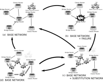
Fig. 1.Typical use case for a base network and a substitution network.

Abstract— A substitution network is a temporary network that self-deploys to dynamically replace a portion of a damaged infrastructure by means of a fleet of mobile routers. In this paper, we evaluate the performance of a previous self-deployment scheme, APOLO, for substitution networks and we show the ben-efit of the controlled mobility in such a network. To that end, we evaluate APOLO in terms of throughput under several scenarios and different metrics. These results constitute a comprehensive evaluation of the adaptive positioning algorithm and enable to envision new ways of optimization and future paths of research.1 Keywords: substitution networks; self-deployment; controlled mobility.

I. INTRODUCTION

A rapidly deployment network is a solution to provide communication services in disaster scenarios. Specifically, we focus on a wireless solution named the substitution networks. A substitution network is a temporary network to replace a portion of a damaged infrastructure (called hereafter base network) by means of mobile routers (called substitution routers) capable of moving on demand and connecting to the

base network through bridge routers (Fig.1a).

1_{This work was partially supported by a grant from CPER CIA and the}

ANR RESCUE project.

Bridge routers are connected in between the base and the substitution networks, and used to forward the traffic from the base network to the substitution network and vice versa.

Mobile substitution routers are wireless routers of the substitution network, possibly connected to bridge routers, and whose union provides alternative path(s) to the base network.

Fig.1 depicts the complete overview of using a substitution

network, where the bridge routers are deployed together with

the base network (Fig.1a). In this example, the base network

operates without the help of the mobile routers. When a failure

occurs (Fig. 1b), the mobile routers are deployed. In this

architecture, the failure detection and the deployment are done autonomously by the base network itself. Mobile routers try to find an optimal position to restore the connectivity service and

to ensure quality of service (QoS) (Fig. 1c). In some cases,

the continuous redeployment of the routers may be necessary

to adapt to evolving network and QoS conditions (Figure1d).

Particularly, our goal is to have an autonomous router

deployment as well asa possible redeployment of the mobile

routing devices. Therefore, it is necessary to design algo-rithms and protocols to deploy and re-deploy such devices. Since the routing devices are autonomously provided with a limited battery, it is also necessary to consider energy constraints during the deployment. Moreover, the deployment computation process does not consider a central entity in the network, hence, this process should be executed in a distributed manner. An efficient router/relay (mobile or static) deployment algorithm must take the link quality into account in order to decide when and where to deploy a relay. For that purpose, the deployment algorithms must be able to measure the wireless link quality. We have presented in a previous work

theAdaptive POsitioning aLgOrithm (APOLO) [1].

This paper presents the extended results of APOLO [1] developed for substitution networks obtained under stress and some results under different assumptions, especially regarding channel states. The remaining of the paper is structured as follows. After browsing the literature (Sec. II), Section III describes the background and the basic concepts used in this paper. Then, Section IV recalls the proposed adaptive positioning algorithm (APOLO). Section V and Section VI present the simulation settings and results. Finally, we discuss these results and conclude in Section VII.

(3)

II. STATE OF THE ART

Mobile routers of a RDN perform the same tasks than their static similar distributing the data traffic, however, they must self-position in a given area. In literature, we find a few relative proposals. [2], presents the Spreadable Connected Autonomic Network algorithm in which the mobile routers move to expand the covered area. In order to maintain the connectivity, they are allowed to move as long as there is no risk of disconnection, if a possible disconnection is detected, the mobile router must stop moving. A different strategy is presented in [3], where the mobile routers follow a leader router in a straight-line formation, once the leader reaches the objective point, it stops and the rest of the routers start stopping. These approaches differ from ours since they do not consider link quality.

III. PRELIMINARIES

We consider a wireless network composed of mobile routers that are located and may move on the two-dimensional Eu-clidean space. We use “node” as a generic term for any device in the simulation neighborhood, for instance, the mobile or classic routers. For the sake of simplicity, we assume that the transmission range R of a node u is the area in which another node v can receive/send messages from/to u, i.e.,

d(u, v) < R(u), where d(u, v) represents the Euclidean distance

between u and v, and therefore, it exists a link X between u and v. We assume that two nodes are “neighbors” when they are within the communication range of each other.

In the following, we use Xprev and Xnextto refer to the links

of the previous and next hops, respectively, of a mobile router. Likewise, we assume that some of the devices are fixed, that traffic needs to be transferred between two fixed devices, and that the wireless routers dynamically move in the scenario and act as relays, regardless of the routing protocol. And, as many link layer protocols, we assume that each node is equipped with a timer and an 802.11 wireless card as well as with an identifier that is unique in the network (MAC address).

We define the quality of communication link, or just “link quality”, as the probability that a message transmitted on the link is successfully received, that is, the reliability of the link [4]. The link quality can be assessed as a function of the received signal strength (RSS) or the signal-to-noise ratio (SNR) [5], for example. In general, higher SNR leads to lower probability of error in the packet. Hence, a link with high SNR

is considered a high-quality link [6]. We use the RSS, SNR,

RTT, and TxRateas values to measure the link quality because

their values retrieve insight of the performance of a wireless network [7]. Therefore, we call RSS, SNR, RTT, and TxRate “link metrics” or “link parameters” in general.

We use the term “broadcast” to refer to the message propagation in a router’s neighborhood in order to obtain the link measurements. Also, we refer to the control packets of routing protocols as “hello” messages or beacons and to the packets used in active measurements as probe packets. Finally,

we define the term controlled mobility as the ability of some nodes to move by themselves to a specific destination or with a specific goal, i.e., the opposite of randomly [8].

In this paper, we use the DSR [9] protocol for our set of

simulations. The DSR protocol is a self-maintaining routing protocol designed for multi-hop wireless networks composed of mobile nodes. DSR uses on demand routing allowing each source to determine the route used to transmit its packets to the corresponding destinations. DSR consists mainly of two mechanisms, Route Discovery and Route Maintenance. Route discovery cycle is used to find a route between the source and the destinations on demand. Route maintenance is used to ensure that the paths remain optimum and loop-free as network conditions change. DSR avoids additional traffic, for example, hello packets by using source routing, i.e., the entire route is part of the packet header and by storing the routes in caches.

IV. ADAPTIVEPOSITIONINGALGORITHM

A new quality-of-service-based architecture for substitution networks presented in [10] envisions a wireless network com-posed of mobile routers/relays that provide alternative paths to the base network. Such substitution routers are able to move on demand, so, they can self-deploy and adapt to the network topology accordingly to the environment conditions.

Previously, we have presented the Adaptive POsitioning aLgOrithm [1] (APOLO) for self-deploying mobile routers in a substitution network. During the substitution network lifetime, APOLO is executed in each mobile router to determine whether it has to move by using the feedback of the link quality coming from one-hop neighbors. APOLO consists of three major stages. Firstly, APOLO measures the link quality by means of one link parameter, e.g., RSSI, SNR, or delay. Secondly, APOLO computes the gathered data and makes the movement decision, i.e., if the router needs to move or not to improve the link quality. And finally, APOLO determines direction of the movement and the router moves accordingly. Results presented in [1], [11] are restricted to only one propagation model (2-ray ground) and 3 simulation scenarios. In this paper, we extend these results with extra propagation models and scenarios. First, we present the results obtained when the router’s initial position is random. Second, we study the behavior of our algorithm when there exist multiple mobile routers between the source and the destination. Then, we evaluate the redeployment capacity of the mobile router when a new node arrives. Finally, we compare the deployment performance of each link parameter under three different propagation models (2-ray ground, shadowing, and ricean).

V. SIMULATION ENVIRONMENT

We present an extension to the experimental performance evaluation of APOLO. Our main goal is to present the effec-tiveness of the algorithm to deploy wireless mobile routers in a given area. To that end, we evaluate our proposal by using

the NS-2 network simulator2_{. In our previous work [11], we}

(4)

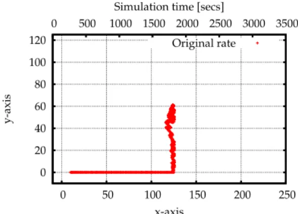
TABLE I.SIMULATION PARAMETERS.

Physical Propagation Two Ray Ground Error Model Real [13] Antennas Gain Gt= Gr= 1

Antennas Height ht= hr= 1 m

Min Received Power Pr−thresh=6.3 nW

Mobile Router Energy 50 J Communication Range 240 m MAC 802.11b Standard Compliant

Basic Rate 2Mbps Auto Rate Fallback 1, 2, 5.5, 11 Mbps LLC Queue size 50 pkts

Policy Drop Tail Routing Static Dijkstra [14]

Routing Traffic None Transport and Flow CBR / UDP Application Packet Size 512 B/1 MB Statistics Number of samples k= 10

Broadcast period t= U (0.1) Mobility Movement step d= 2m

have chosen three scenarios proposed in [12] as a result of the study on relay wireless networks. We propose three additional scenarios plus a propagation model comparison.

Since our goal is to assess the impact of controlled mobility in wireless routers, we use the Dynamic Source Routing (DSR) protocol for our simulations, although, APOLO is not tied to any routing particular protocol. Table I summarizes the basic parameters used in our simulations in NS-2. In this paper, we

use the instantaneous throughput (THins) defined as he number

of bits transferred to the final destination in any given instant to assess the performance of our deployment algorithm.

VI. RESULTS

A. Random initial position

In our previous work, the basic scenario is composed of one mobile router, one source node (S), and a destination node (D). The source and the destination are placed 250 m away from each other, i.e., the source is placed at coordinates (0,0) and the destination at coordinates (250,0). Finally, at the beginning of the simulation, the router node is placed 10 m away from the

source node, that is, at coordinates (10,0) as depicted inFig.2.

Then, the router starts moving based on APOLO. Nevertheless, the mobile router may reach the position that equalizes the parameter values regardless of its initial position.

Hence, we take again this basic scenario. We run a set of simulations choosing the initial position of the router randomly. We use the 802.11b standard along with the

two-ray ground model.Fig.3 plots the x coordinates along time to

illustrate the movement evolution.Fig.3(a) presents the results

S D

Fig. 2. Basic scenario composed of one mobile router, one source node, and one destination node.

0 200 400 600 800 1000 0 50 100 150 200 250 Simulation time [s]

Distance from the source [m]

Router 1 0 200 400 600 800 1000 0 50 100 150 200 250 Simulation time [s]

Router 1

(a) Results by using the RSS as link metric 0 200 400 600 800 1000 0 50 100 150 200 250 Simulation time [s]

Router 1

(b) Results by using the SNR as link metric

Fig. 3. Simulation results for random initial position of the mobile router.

while using the RSS as link metric andFig.3(b) presents the

results while using the SNR as link metric. In Fig. 3(a) the

router’s initial coordinates are (23,0), (128,0), and (160,0), respectively. The theoretical position that equalizes should be (125,0) where the router is placed at exactly the middle point between the source and the destination, and therefore,

the link values of Xprev and Xnext should be the same. We

observe in Fig. 3(a) that the router reaches such a position

regardless of its initial position, an expected result since the two-ray ground model calculates the RSS as a function of the

distance. Similarly, inFig.3(b) the router’s initial coordinates

are (42,0), (147,0), and (206,0), respectively. Despite the router does not reach a steady position, this behavior corresponds to the previous simulations where the router’s initial position is (10,0), in other words, the initial position of the router does not affect the movement behavior by using SNR as link metric. We believe that such a behavior is due to the propagation model we have used. In order to corroborate this, we perform a set of simulations with different propagation models. The results are presented in Section VI-E.

B. Multiple routers scenario

In [11], we study the performance of APOLO by consid-ering a scenario with two routers. In such a scenario, there is a source and a destination communicating though two mobile routers, so, we extend this scenario by considering three and four intermediate routers between the source and

(5)

1) Three routers: Regarding the three router scenario, the source, once again, is placed at coordinates (0,0) and the destination at coordinates (300,0), that is, 300 m away from each other. At the beginning of the simulation, Router 1 is placed at coordinates (10,0), Router 2 is placed at (150,0), and Router 3 is placed at (290,0). Then, the routers execute APOLO to adjust their position using the RSS as link metric,

the results are presented inFigure5. The deployment evolution

is plotted as x coordinates as function of simulation time where we observe that the behavior of the routers follows the results

obtained with the two router scenario (Figure5(a)). The routers

travel the corresponding distance to equalize the values of the link metric. In this case, Router 1 and Router 3 travel a similar distance. The routers reach their final position after 550 s, which are, Router 1 at 75 m, Router 2 at 150 m, and Router 3 at 225 m from the source, that means a distance of

75 m between each node.Figure 5(b) plots the instantaneous

throughput obtained during the routers deployment.

2) Four routers: Regarding the four router scenario, the

source is placed at coordinates (0,0) and the destination at coordinates (400,0), that means, 400 m away from each other. At the beginning of the simulation, Router 1 is placed at coordinates (10,0), Router 2 is placed at (140,0), Router 3 is placed at (260,0), and Router 4 is placed at (390,0). Subsequently, each router adjusts its own position by executing

APOLO using RSS as link metric. Figure 6(a) shows the

routers deployment through the simulation time. Once again, the final position of the routers equalize the link metric and it is equidistant between nodes. These results, three and four routers, show that the behavior experienced with only one mobile router is duplicated, and therefore, APOLO is a scalable solution and it is able to deal with multiple router scenarios.

C. Two sources and one destination scenario

By the same token, we evaluate APOLO in a multiple destination scenario [1]. In addition, we present a topology

S D

Fig. 4. Multiple routers scenario composed of three mobile routers, one source node, and one destination node.

0 200 400 600 800 1000 0 50 100 150 200 250 300 Simulation time [s]

Router 1 Router 2 Router 3

(a) Movement evolution in time of the mobile routers

0 200 400 600 800 1000 0 200 400 600 800 1000 1200 1400 1600 1800 Simulation time [s] Throughput [kbps] Instantaneous Throughput

(b) Throughput as a function of time Fig. 5. One source, one destinations, and three mobile routers.

0 200 400 600 800 1000 0 50 100 150 200 250 300 350 400 Simulation time [s]

Router 1 Router 2 Router 3 Router 4

(a) Movement evolution of the routers 0 200 400 600 800 1000 0 200 400 600 800 1000 1200 1400 1600 Simulation time [s] Throughput [kbps] Instantaneous Throughput

(b) Throughput as function of the time

Fig. 6. Multiple routers scenario composed of four mobile routers, one source node, and one destination node.

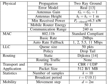
Fig. 7. Two sources, one destination, and one mobile router scenario.

with multiple sources by using the topology depicted in

Figure 7, where we illustrate two sources (n0, n1) and one

destination (n3) out of range. Thus, a mobile router (n2) is used to connect the sources and the destination. At the beginning of the simulation, the router (n2) is placed 10 m away from the source nodes (n0, n1) on the straight line that connects the sources from the middle position between the receiver node (n3), and finally, we use User Datagram Protocol packets with a size of 1 MB since UDP is used in most multimedia applications.

In this scenario, two identical CBR/UDP flows are trans-mitted from the source nodes (n0, n1) to destination node (n0) starting and finishing at the same time. A priori, we assume that the best position is located at the coordinates (83,125), which is the triangle centroid. Then, the router uses APOLO to decide where to move and RSS as link metric.

The movement trace is depicted in Figure 8(a). During the

first 500 s, the router moves in a straight line from (10,125) to (94,125), i.e., it travels 84 m. After this time, the router moves from left to right (in the y axis domain) in a range of ±3 m, i.e., from (94,128) to (94,122). This behavior is very different from that one experimented in a similar scenario with two source nodes and one destination. In the latter scenario, the router moves mostly in the x axis range and stops very close to the triangle centroid. Hence, the oscillation experienced in two source scenario is caused by the two flows arriving to the router, that means, the router moves to improve the link quality

(6)

0 20 40 60 80 100 121 122 123 124 125 126 127 128 129 x position [m] y position [m] Router 1

(a) Movement evolution of the router

0 1000 2000 3000 4000 0 500 1000 1500 Simulation time [s] Throughput [kbps] Instantaneous Throughput

(b) Throughput as function of the time

Fig. 8. Scenario two sources and one destination. Movement of the mobile router through the time and the corresponding throughput.

accordingly to the data flow arriving at the time. In order to avoid wasting energy with short distance movements, it is possible to implement a movement threshold, for example, the router moves if the RSS value drops under certain threshold. D. Redeployment

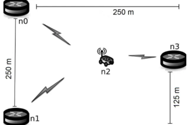
One issue that remains open is the routers redeployment. The redeployment is specially important in dynamic scenarios. In the following, we present a simulation campaign where the redeployment is needed. As in the previous set of simulations, the mobile router executes APOLO to redeploy and uses RSS as link metric. At the beginning of the simulation, the

scenario is the one depicted inFigure2, one source node, one

destination node, and one mobile router. The source (n0), the router (n1), and the destination (n2) are located at coordinates (0,0), (10,0), and (250,0), respectively. Then, after 650 s a new source node (n3) arrives to transmit data to (n2), and therefore, the router must adapt its position. Node (n3) appears at coordinates (0,125).

Figure 9 plots the movement of the router in the Cartesian space. The first seconds of the simulation, the router follows the same behavior than in the previous simulation, in other words, the router reaches the position at (125,0). Then, when the second source appears, the router starts to move to equalize the quality of the new link between (n3) and (n1). Finally, the router reaches its final position at coordinates (124,60). These results are very interesting for two reasons. Firstly, they prove that APOLO is useful to redeploy automatically mobile routers, and hence, it is well suited in dynamic scenarios. And secondly, the results prove the importance of the hello messages to advertise the eventual changes in the network topology, if the transmission rate of such hello messages is too low, the information gathered may not reflect the changes in the topology over the time. Nevertheless, it is also important to consider the cost of such hello messages in terms of energy and overhead. To overcome this problem, it is interesting to study

the optimal transmission frequency of the hello packets [15]

as well as the overhead reduction techniques.

E. Propagation model comparison

The propagation models are empirical mathematical formu-lations to characterize the radio wave propagation based on

0 20 40 60 80 100 120 0 50 100 150 200 250 0 500 1000 1500 2000 2500 3000 3500 y-axis x-axis Simulation time [secs]

Original rate

Fig. 9. Redeployment of a mobile router.

physical phenomena such as distance, used frequency, or fad-ing effects. In wireless network simulations, the propagation models are used to simulate the wireless channel by computing the wireless signal strength at the receivers for any packet transmitted by a single sender. Particularly, NS-2 simulator provides three propagation models: Free space model, Two Ray Ground model, and Shadowing model. Moreover, it is

possible to add a fourth model called Ricean3.

Each propagation model computes the attenuation of the signal strength between the sender and the receiver by using a Carrier Sensing Threshold (CSThresh_). If the signal strength is lower than CSThresh_, the packet is discarded at the physical layer. Otherwise, the signal strength is compared to a second threshold at the receiver (RxThresh_) to determine whether the packet is received with errors or not. If so, the MAC layer discards the packet.

Free space model represents the transmission range as a perfect circle around the sender. Basically, if the receiver is within the circle, it will receive all the packets; otherwise, it loses them. Two-ray ground reflection model considers both the direct path and a ground reflection path, a difference from the free space model, which only considers a single line-of-sight path. The two-ray ground model gives more accurate prediction at a long distance than the free space model. Nevertheless, the free space model is used when the distance is small because the two-ray model does not give a good result for a short distance due to the oscillation caused by the constructive and destructive combination of the two rays. It is important to notice that both models represent the communication range as a prefect circle, i.e., the received power is a deterministic function of distance. On the other hand, the shadowing model takes the fading phenomenon into account. Finally, the Ricean model characterizes the effect of small-scale fading (Rayleigh and Ricean). Such a fading is caused by movement of the sender, receiver, or of other objects in the environment. This movement may be characterized by the Doppler spreading.

As in the previous sections, we evaluate the performance 3_{http://www.isi.edu/nsnam/ns/doc/node216.html}

(7)

0 50 100 150 200 250 0 200 400 600 800 1000 1200 1400 1600 1800 2000

Simulation time [s] Ricean propagation model

RSS SNR TR 0 50 100 150 200 250 0 200 400 600 800 1000 1200 1400 1600 1800 2000

Simulation time [s] Shadowing propagation model

RSS SNR TR 0 50 100 150 200 250 0 200 400 600 800 1000 1200 1400 1600 1800 2000

Simulation time [s] Two ray ground propagation model

RSS SNR TR

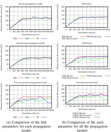
(a) Comparison of the link parameters for each propagation

model. 0 50 100 150 200 250 0 200 400 600 800 1000 1200 1400 1600 1800 2000

Simulation time [s] RSS-based RSS-Ricean RSS-2RayGround RSS-Shadowing 0 50 100 150 200 250 0 200 400 600 800 1000 1200 1400 1600 1800 2000

Simulation time [s] SNR-based SNR-Ricean SNR-2RayGround SNR-Shadowing 0 50 100 150 200 250 0 200 400 600 800 1000 1200 1400 1600 1800 2000

Simulation time [s] Transmission rate-based

TxRate-Ricean TxRate-2RayGround TxRate-Shadowing

(b) Comparison of the each parameter for all the propagation

models.

Fig. 10. Evaluation of APOLO under different propagation models. The movement of the mobile router as function of time.

of APOLO under three different propagation models, Ricean, Two ray ground, and Shadowing. To that end, we use the

one source-one destination scenario (Figure 2), the router is

placed at coordinates (10,0). Then, we vary the propagation model for each of the link parameters, i.e., RSSI, SNR, RTT, and transmission rate. The results obtained are presented

in Figure 10. Figure 10(a) presents the comparison of the

router deployment by using all the APOLO variants for each model propagation. The Two-ray ground plot was presented in [1], where router using the RSS variant reaches exactly the middle point between the source and the destination, i.e., at coordinates (125,0) while the router using the SNR and TxRate does not reach a steady point. However, this behavior changes completely when we evaluate APOLO by using the Ricean and Shadowing models. Under both models, Ricean, and Shadowing the performance of the three variants is similar. None of the variants reaches a steady point still the router moves ±10 m away from the middle point (125,0). Nonetheless, this behavior confirms our observation about the SNR performance obtained in Section VI-A, that is, since each propagation model characterizes in different way the events at the physical layer, the values of the link metrics correspond to such characterization and behave accordingly. We also include a comparison of each link parameter under all the propagation models to clarify the difference in the behavior

(Figure10(b)). Because the link quality values depend largely

on the propagation model, it is important to choose the one

that characterizes better our case of study. In general, the NS-2 community uses the two ray ground model but the shadowing model corresponds better to the real scenarios.

VII. CONCLUSION ANDFUTUREWORK

We have presented the impact of controlled mobility to self-deploy routers in substitution networks. The results provide a wider view of the performance of the Adaptive POsitioning aLgOrithm (APOLO). They prove that APOLO is able to successfully deploy the mobile routers in several scenarios and by using different propagation models. Even more, APOLO performs well also when router redeployment s needed.

We observed that by using the Ricean and Shadowing models the deployment performance of the SNR and TxRate variants outperform the two-ray ground one even if in the former case the router does no reach a steady point. This disadvantage may be overcome by adding a threshold to avoid useless movements. Thus, we are interested in studying how the threshold choice may (or may not) impact the performance.

REFERENCES

[1] K. Miranda, E. Natalizio, and T. Razafindralambo, “Adaptive Deploy-ment Scheme for Mobile Relays in Substitution Networks,” International Journal of Distributed Sensor Networks (IJDSN), 2012.

[2] J. Reich, V. Misra, D. Rubenstein, and G. Zussman, “Connectivity Maintenance in Mobile Wireless Networks via Constrained Mobility,” IEEE JSAC, vol. 30, no. 5, pp. 935–950, Jun. 2012.

[3] C. Q. Nguyen, B.-C. Min, E. T. Matson, A. H. Smith, J. E. Dietz, and D. Kim, “Using Mobile Robots to Establish Mobile Wireless Mesh Networks and Increase Network Throughput,” IJDSN, vol. 2012, pp. 1–13, 2012.

[4] M. R. Souryal, A. Wapf, and N. Moayeri, “Rapidly-Deployable Mesh Network Testbed,” in Proc. Globecom, Honolulu, USA, 2009. [5] N. Baccour, A. Koubaa, H. Youssef, M. Ben Jamâa, D. do Rosário,

M. Alves, and L. Buss Becker, “F-LQE: A Fuzzy Link Quality Estimator for Wireless Sensor Networks,” in Proc. of EWSN, Coimbra, Portugal, 2010.

[6] S. Farahani, ZigBee Wireless Networks and Transceivers. Newton, MA, USA: Newnes, 2008.

[7] E. Feo Flushing, J. Nagi, and G. A. Di Caro, “A mobility-assisted protocol for supervised learning of link quality estimates in wireless networks,” in Proc. of ICNC, Maui, Hawaii, USA, 2012.

[8] E. Natalizio and V. Loscrì, “Controlled mobility in mobile sensor net-works: advantages, issues and challenges,” Telecommunication Systems, vol. 52, no. 4, pp. 2411–2418, Apr. 2013.

[9] D. B. Johnson, D. A. Maltz, and J. Broch, “Ad Hoc Networking.” Addison-Wesley Longman Publishing Co., Inc., 2001, ch. DSR: The Dynamic Source Routing Protocol for Multihop Wireless Ad Hoc Networks, pp. 139–172.

[10] T. Razafindralambo, T. Begin, M. Dias de Amorim, I. Guérin Lassous, N. Mitton, and D. Simplot-Ryl, “Promoting Quality of Service in Substitution Networks with Controlled Mobility,” in ADHOC-NOW, Paderborn, Germany, 2011.

[11] K. Miranda, E. Natalizio, T. Razafindralambo, and A. Molinaro, “Adap-tive router deployment for multimedia services in mobile pervasive environments,” in Proc. WIP of PerCom, Lugano, Switzerland, 2012. [12] L.-L. Xie and P. Kumar, “Multisource, Multidestination, Multirelay

Wireless Networks,” IEEE Transactions on Information Theory, vol. 53, no. 10, pp. 3586–3595, Oct. 2007.

[13] J. del Prado Pavon and S. Chio, “Link adaptation strategy for IEEE 802.11 WLAN via received signal strength measurement,” in Proc. of ICC, Anchorage, USA, 2003.

[14] E. Dijkstra, “A note on two problems in connexion with graphs,” Numerische Mathematik, vol. 1, no. 1, pp. 269–271, 1959.

[15] X. Li, N. Mitton, and D. Simplot-Ryl, “Mobility Prediction Based Neighborhood Discovery in Mobile Ad Hoc Networks,” in Proc. of the 10th Networking Conference (NETWORKING), Valencia, Spain, 2011.