HAL Id: hal-01896681
https://hal.archives-ouvertes.fr/hal-01896681
Submitted on 4 Mar 2021
HAL is a multi-disciplinary open access
archive for the deposit and dissemination of
sci-entific research documents, whether they are
pub-lished or not. The documents may come from
teaching and research institutions in France or
abroad, or from public or private research centers.
L’archive ouverte pluridisciplinaire HAL, est
destinée au dépôt et à la diffusion de documents
scientifiques de niveau recherche, publiés ou non,
émanant des établissements d’enseignement et de
recherche français ou étrangers, des laboratoires
publics ou privés.
To See or Not To See: Determining the Recognition
Threshold of Encrypted Images
Heinz Hofbauer, Florent Autrusseau, Andreas Uhl
To cite this version:
Heinz Hofbauer, Florent Autrusseau, Andreas Uhl. To See or Not To See: Determining the Recognition
Threshold of Encrypted Images. 7th European Workshop on Visual Information Processing, EUVIP,
Nov 2018, Tampere, Finland. �10.1109/EUVIP.2018.8611779�. �hal-01896681�
To See or Not To See: Determining the Recognition Threshold
of Encrypted Images
Heinz Hofbauer
University of Salzburg Department of Computer Sciences
hhofbaue@cosy.sbg.ac.at
Florent Autrusseau
Inserm, UMR 1229, RMeS Regenerative Medicine and Skeleton University of Nantes, ONIRIS France Florent.Autrusseau@univ-nantes.fr
Andreas Uhl
University of Salzburg Department of Computer Sciences
uhl@cosy.sbg.ac.at
Abstract—There are numerous standards and
recommen-dations when it comes to the acquisition of visual quality assessment from human observers. The recommendations deal with clearly visible images and try to keep the just-noticeable-difference between quality steps as small as pos-sible to facilitate an exact measurement of image differences. When it comes to the assessment of selective encryption schemes the question is the opposite. The quality is not really of interest, the question is rather if the content of the images is discernible at all. There are no recommendations in literature for this kind of task. In this paper we will outline different protocols and setups, test them and form a recommendation for the acquisition of the recognition threshold for encrypted images from human observers.
I. Introduction
Selective encryption (SEnc) is the encryption, utilizing state of the art ciphers like AES, of a selected part of a media file or stream. The goal is to secure the content, or parts thereof, while still maintaining the file format, that is the file is still usable as the media file or stream it actually is.
When it comes to recognizing content there are various target levels in terms of quality: transparent encryption wants to reveal a low quality version of the content, e.g., as a preview, sufficient
encryption wants to reduce the content to a level where a
consumption of the image or video is no longer possible but does not care if potential content is leaked, e.g., consumers still recognize what is going on in a movie but the quality is so low that a pleasurable viewing experience is prevented (pay-per-view scenarios). Confidential encryption is the next step where the goal is to actually make the content of the data unrecognizable.
There are numerous SEnc encryption schemes, e.g., [1, 2, 3, 4], and an important assessment is always that of quality and recognizability. It has been pointed out, [5], that the quality assessment is problematic since quality metrics are not usually built for such low quality material. The same paper also points out that the automatic assessment of recognizability is not possible since there are no metrics, databases or methods for the generation of such databases in literature.
This is indeed our goal in this paper, we aim to produce a set of guidelines for the acquisition of information pertaining to the recognition threshold. That is, the threshold where the encryption is so strong that it crosses from a low quality but recognizable image/video to a image/video where the content is no longer recognizable.
This can be formulated slightly differently, and in the style of indistinguishability under chosen-plaintext attacks (IND-CPA), as: When presented with both encrypted and non-encrypted data, can one be mapped to the other?
We will present different methods to acquire the recogni-tion threshold and compare them. Furthermore, we will look at recording conditions, which might influence the ease and quality of the acquired data, by starting with recommendations for image quality evaluation tests, with very strict illumination restrictions, to less controlled environments.
We will introduce these methods, environments and the reasoning for them in Section II. In Section III we will describe and perform the experimental analysis of the proposed methods and discuss the findings. Section IV will recap the findings and conclude the paper.
II. On the Acquisition of the Recognition Threshold for Encrypted Images
The VQEG and ITU groups regularly issue recommendations [6, 7, 8, 9] concerning the subjective setups and protocols. There are numerous protocols and each one is adapted to a partic-ular viewing task or image processing method. For instance, ACR (Absolute Category Rating), DSIS (Double Stimulus Impairment Scale) or DSCQS (Double Stimulus Continuous Quality Scale) protocols can be used to rate the quality of an encoding (compression) method. The Two Alternative Forced Choice (2AFC) protocol is commonly used to track a visibility threshold, and can thus be used in a data hiding framework.
Further, there are recommendations for the subjective test setup which should adhere to several basic rules. The screen should be calibrated, its luminance must be controlled. Sur-rounding illumination has to be limited. The viewing distance, the experiment duration, the observers’ acuity, are among the parameters that must be controlled.
In this section we will discuss the acquisition method (pro-tocol) and environment and the differences in assessment of quality and recognizability with the goal of evaluating different modalities to find the easiest setup, in terms of practicality, which still yields high quality results. Finally we will discuss the handling of outliers and generation of a recognizability score based on the acquired data.
A. Protocols for Acquisition
What we want to acquire is a score per image which reflects the recognizability of it’s content. This score should ideally be on a continuous scale so that we can track the transition from recognizablity to unrecognizability.
The regular acquisition methods for quality estimation of im-ages are not applicable to finding the recognizability threshold. The question is not how good the quality is but rather: Is the
basic transference of the methodology from quality assessment would be to present an original and an encrypted image and ask the user whether or not information from the original image is still retained in the encrypted image. This approach suffers from apophenia, the tendency to perceive connections and meaning between unrelated things.
To prevent this, a forced choice is suggested, where the participant has to choose among a number of candidate images and identify the “correct” one. If the contents of an image is truly not recognizable then the participant has to guess. In other words the ratio of observers which correctly identify the image will tend towards the probability of random choice.
Three methods are conceivable, and will be tested in the experimental section.
1) O3: Show a single original image and three encrypted im-ages. The participant has to select the encrypted version of the original image.
2) 3E: Three plain text images and one encrypted image is shown. The participant has to select the correct original image from which the encrypted image was derived. 3) Match2: Three originals and three encrypted images are
shown. One pair of images is an original and derived encrypted image, the other four images have to be un-related. The participant must select the matching pair. The way these protocols display images is shown in Figure 1. The reason the Match2 variant is used is that the one vs. three methods might allow for exclusion type strategies where images can be disregarded leading to a possible skew in probability. In the long run this phenomenon should even out but it might lead to a higher number of required participants for that to happen.
For all three methods it is required to have images with similar encryption strengths to be shown simultaneously.
B. Environment for Acquisition
The environment in which to perform quality assessment is regulated by standards, e.g., ITU-R BT.500-13 [10]. The standards are aimed at high quality tests and generating an environment where the just noticeable difference in images is as small as possible to enable an optimal quality assessment. Even for quality assessment, strictly following these standards can be called into question in part due to recent experiments. When building the TID database [11, 12], laboratory setting were conform to ITU-R BT.500-13 [10] and an off-site environment (via internet) was used as well. The resulting data exhibited no conspicuous disagreement.
A less stringent control over the environment clearly leads to a easier and more manageable set up of experiments which would allow easier acquisition of datasets to help in research, as long as the quality of the acquired data does not suffer.
The need for the use of strictly constrained subjective en-vironment setups may make sense when the subjective task is to score the quality of slightly distorted images/videos, or when the task is to track a visibility threshold (such as in a data hiding framework). However, in the context of recogni-tion of selectively encrypted images, where the task is not to adjudicate a minute difference in quality but to decide if two images contain the same content, the viewing conditions may not significantly influence the results.
In order to evaluate the environmental influence on the recording we will utilize three different setups:
1) Controlled (CE): The controlled environment uses a calibrated monitor in a closed room, i.e., no natural light-ing is present, and a strictly controlled artificial lightlight-ing to conform to ITU-R BT.500-13 [10].
2) Semi-controlled (SE): A regular working space, some measures were taken to limit extraneous light, e.g., blinds were drawn.
3) Uncontrolled (UE): The uncontrolled environment is simply what was available at the users own PC. The experiment was set up to be used over the internet at the workstation of the users PC.
Viewing distance: In both the CE and SE, a supervisor instructed the observer to keep a proper viewing distance. The viewing distance was set to 6 times the images’ height.
Scaling: Controlled and semi controlled environment have screens which are sized so that the images are not scaled. The uncontrolled environment scales down if necessary to display the 6 images in the 3x2 configuration but will not scale up.
Illumination and Calibration: Optimally a controlled environment and a high quality calibrated monitor is recom-mended. The specs in the CE were: illuminant white point
CIE D65, maximum screen luminance of 200 cd/m2, screen
gamma function of 2.20, contrast ratio/ black point of 2 cd/m2
and background illumination of 10 lux. Our setup was thus compliant with the recommendations of ITU-T REC P.910 [13], ITU-R BT.500-11 [14] and ITU-R BT.500-13 [10].
Viewing Time: We restricted viewing time to prevent a timely conclusion, which is important for the acquisition of large amounts of data. The viewing time restriction also serves to prevent fatigue for the observers. The time chosen was
8 seconds in opposition to the recommended 10 sec
(ITU-R BT.500-11 [14]). The reasons for this are twofold: 1) the recognizability framework is easier than quality assessment and consequently takes less time and 2) it allows for more com-parison before observer fatigue sets in which is an important practical consideration. We did not control for time in the uncontrolled environment.
Vision Check: For the CE environment a proper vision test was performed: Observers were screened to ensure perfect visual acuity and detect possible color deficiencies. The Snellen eye chart was used to control the acuity, and the Ishihara color plates were used to validate a normal color vision. For the SE setup the means were more limited but we utilized an online vision test to check visual acuity, near vision and color vision. No vision check was performed for the uncontrolled environment.
Number of Observers: The minimum number of observers recommended by all standards is 15 and was exceeded in all environments.
The conformance of the various environments to the sug-gested setup of the standards as described above is summarized in Table I. The experiment of the acquisition protocol uses the
UE setup from the table but we could only procure sixteen
observers for this test.
C. Analysis of Data
The handling of the data is also somewhat different from usual quality experiments. The main difference is that during quality evaluation each observer gives a rating for each image. Based on these ratings the outliers can be detected. For each recognition task, the observer only generates a binary output,
O3 3E Match2
Fig. 1. Examples of the O3, 3E and Match2 protocols for the recognizability test. TABLE I
Conformance to constraints by the acquisition environments.
Lumi- Viewing Scale Vision View Observ-nance Distance Check Time ers
CE 3 3 3 3 8 sec 45
SE 7 3 3 ∼ 8 sec 30
UE 7 7 7 7 ∞sec 41
content recognized or not. The final score is an aggregate over all observers, and is expected to trend towards the randomness in case of unrecognizability. The probability of a randomly
correct guess ( pr) depends on the setup, each choice of images
is one in three resulting in pr
3E = p r O3 = 1 3 = 0.3 ˙3, and pr Match2= 13 1 3 = 0.1 ˙1.
Outlier detection: Outlier detection in the classical sense will not work, since the data being collected are not numerical scores, but rather some binary information representing correct or incorrect recognition. A simple error aggregate also won’t work since two observers can have the same number of errors while not agreeing on a single image. Given that we have essentially a vector with binary values the Hamming distance comes to mind, then we can at least compare two observers and get a meaningful score. An outlier in this context can then be seen as an observer whose opinions strongly differ from the majority of the other observers. To find outliers we can perform a hierarchical clustering which starts with the smallest distance and continues to cluster the elements together until a single cluster has formed. The outliers can then be detected based on statistics of similarity between observers like so: with O the set
of observers and D = {HD(Oi, Oj) | ∀Oi, Oj∈ I, i 6= j}the set
of pairwise distances we use the z-score zD= µ(D) + 3σ(D)to
find observers which are very far from the group consensus. Depending on the aggregation of clustering it might be useful
to use the `1 measure as a generalized version of the Hamming
distance, as long as no merging of vectors is performed, i.e., if
for a vector v, vi∈ {0, 1}, i = 1, . . . ,#v holds, then kv −wk1=
P#v
i=0|vi− wi| =P#vi=0vi⊕ wi= HD(v, w), with #v being the
dimension of the vector v (and w). This method might however be useful if a different clustering or aggregation method is used. As aggregation of cluster size, and distance to cluster cal-culation, it is suggested to use the maximum over all pairwise distances. That means that all pairwise distances in the cluster
are below the chosen threshold zD= µ + 3σ.
The way this looks in practice can be seen in Figure 5 later in the paper. The clustering is displayed as a dendrogram, a tree of merge decisions, the y-axis gives the merges at the height of the new cluster size. If the tree is cut off at a height matching
zD it will split into sub clusters where each cluster does not
contain outliers. The largest such cluster is then used as the
“correct” set of observers, the others are considered outliers (marked in red in the dendrograms).
III. Experiments
We have set up experiments to evaluate the different methods of acquisition and environments as specified in Section II. We will analyze the setups and results and try to give recommen-dations if more than one method was proposed.
The database of encrypted images: Figure 2 shows sam-ples of encryption for one method and image to give the reader an idea about the makeup of the database. We used images from
the Kodak database1 having a landscape format, specifically
images numbered 6,8,13,14,16,21,23,24 (reduced data set). This was augmented in later stages with images id, 11, 20, 22 from the Kodak database, furthermore gray-scale versions of images number 23 and 24 as well as a Philips PM5544 test
pattern2 cropped to the Kodak image size were included. This
extended data set was used later in the test when the setup was fixed and a larger data set could be accommodated due to a more limited number of experiments.
A Note on the Datasets: The choice of data set in our case was to use images which are known in the vision community. Since SEnc strongly depends on the content of the image and the algorithm used we decided to also include the Philips PM5544 test pattern since it contains blocks of color and frequency information and allows a more clean separation of content type than a natural image.
It is interesting to notice that the recognizability rate strongly depends on the image content. For instance, all images in Figure 3 are encrypted with the same parameters, but, as can be observed, this induces very different recognizability rates, also reported in the figure. The color patches influence the recognition, as observed in the third row of Fig. 3. While the influence of uniformly colored areas is clearly apparent in the third image it can also happen in natural images, as exemplified in the second row where uniform dark areas remain visible. For the generation of a testset it is therefore recommended to also include artificial images, like the test pattern, which allow for the clear identification of the process leading to a higher recognition rate. While such circumstances can be deduced from natural images as well, row two, it is a far simpler task when the results are as clear as the example in the third row.
A Note on the Encryption: To describe the three en-cryption methods, [2, 3, 4], used would only clutter the paper without giving any new insight. It should suffice that the encryption strength ranges from a relatively high quality to a non recognizable quality, illustrated in Fig. 2 and 3.
1http://r0k.us/graphics/kodak/index.html
2https://commons.wikimedia.org/wiki/File:PM5544_with_
Fig. 2. A sample from the database (Kodak #24): the original image and it’s encrypted variants for one of the encryption methods.
(a) image 3 (b) image 7 (c) Philips PM5544
(d) RE = 0.874 (e) RE = 0.329 (f) RE = 0 Fig. 3. Original images (top), along with their encrypted version (bottom) using the same encryption parameter, recognition errors (RE) are also given per image.
A. Evaluation of the Acquisition Protocol
Three layouts were tested, O3, 3E and Match2, as described in Section II-A and illustrated in Fig. 1.
A web-based version of the experiment was tested with six-teen observers. The tests were conducted in normal office/home viewing conditions, i.e. varying sunlight illumination, various screen resolutions, uncalibrated monitors, varying viewing dis-tances, in essence similar to the UE setup.
The experiment was composed of 8 images (reduced data set), each one being distorted with a single encryption method with 6 different encryption parameters, thus composing a dataset of 56 images. The collected outputs were the number of mis-detections. In Figure 4, we show how the detection errors were distributed across the three setups. Overall, the decision appeared to be more difficult for the Match2 protocol.
M is se d d et ec ti o ns 0 5 10 15 0 5 10 15 Experiments O3 3E Match2
Fig. 4. Repartition of the mis-detections across the three pre-tests.
Our goal is to collect a set of recognizability scores that will be continuously distributed. The recognizability score is in essence the percentage of observers who recognized the content. If the decision process is too simple, few if any errors will happen and the resulting score will almost be binary. This would allow us to state that there are recognizable and unrecognizable images, but not what happens between these
two states. A result that is continuous allows us to perform research at the transition from recognizable to unrecognizable. Match2 spans a wider range of missed detections, resulting in more errors and a higher number of scores which are between recognizable/nonrecognizable. More errors allow for a better approximation of a continuous score, insofar as that is possible with a countable number of observers.
This work is part of a wider project, where the aim is not only to design the best subjective protocol for a recognizability task (work presented in this paper), but we also plan to compare recognizability to a regular quality assessment task. Moreover, in future works, we aim to determine the Objective Quality Metric that will best predict the recognizability. Thus, in order to reach these goals, we need to collect a subjective dataset which is focused onto the transition from unrecognized to recognized content (the slope of the curves in Fig. 7).
B. Evaluation of the Acquisition Environment
The Match2 protocol was chosen based on the results from the previous section. The setup follows the considerations in section II-B. Due to the resolution of the selected images (768×
512pixels), in order to be able to display three images side by
side on the screen, a Wide Quad High Definition (2560 × 1440) monitor was used for the setups CE and SE. The resolution for UE could not be controlled, but the resolution of the web application was reported, as explained later.
For this experiment we increased the number of images in the test set (extended data set) and used two encryption methods (testset 1 and testset 2), again with 6 impairment steps for a total of 182 images. Table I lists the various settings and constraints of each experiment. The same number of observers was used on testset 1 and 2 in each environment.
For the CE the following statistcics were additionally gath-ered: Except 3 observers who had a 20/25 vision, all other observers had at least a 20/20 acuity according to the Snellen chart. Only one of these observers (with a 20/25 acuity) was discarded during the outliers detection step. Three observers had a red/green color deficiency (none were discarded).
1) Outlying Observers Detection: After running a
subjec-tive experiment, during the data analysis step, we inevitably encounter discrepancies in the data. For a high number of observers this will statistically even out, but for a smaller number of observers outliers can significantly skew the results. Therefore, it is best to remove outliers before drawing results from the data gathered. We utilize the clustering outlier detec-tion (dendrograms) as specified in Secdetec-tion II-C.
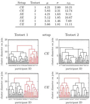
Table II shows the result of the clustering based outlier detection for the three setups and Figure 5 illustrates the clustering and outlier cutoff as dendrograms. Note that the dendrogram for SE is not shown as there were no outliers for these two experiments.
As can be seen in Figure 5 there is a significant variation in the number of outlying observers regarding the various setups.
TABLE II
Distribution of observer difference and resulting threshold zD and outliers for the three acquisition
environment experiments per testset. Setup Testset µ σ zD CE 1 4.21 2.00 10.21 CE 2 5.83 2.31 12.74 SE 1 4.21 1.63 9.11 SE 2 5.12 1.85 10.67 UE 1 3.31 1.46 7.69 UE 2 5.66 1.81 11.11
Testset 1 setup Testset 2
11 16 28 14 13 20 27 38 45 22 30 31 8 34 36 4 15 40 1 37 3 25 24 26 17 10 42 18 35 6 29 32 23 43 33 39 5 12 21 44 2 9 19 7 41 0 5 10 15 20 participant ID cluster diameter on join CE 28 7 9 6 4 32 45 38 39 8 11 40 41 44 12 37 21 23 34 29 27 25 13 14 10 26 15 22 35 43 1 33 20 42 16 30 3 2 24 36 18 5 19 17 31 0 5 10 15 participant ID cluster diameter on join 25 18 38 9 34 1 5 21 40 27 2 24 29 19 20 28 23 30 39 7 32 22 37 26 35 12 3 11 4 6 16 31 33 17 36 8 41 10 14 13 15 0 5 10 15 participant ID cluster diameter on join UE 14 33 16 29 27 20 4 23 32 39 25 26 28 8 17 12 41 35 18 30 3 5 13 21 31 15 36 9 1 24 34 37 40 19 38 10 22 11 6 2 7 0 2 4 6 8 10 participant ID cluster diameter on join
Fig. 5. Dendrograms of the hierarchical clustering, outlier branches are shown in red. Two testsets were evaluated for each environment.
This variation can be explained by the different populations that were enrolled for the tests. The observers in the SE ex-periment were computer scientists , a large part of the observer pool was familiar with the chosen contents (Kodak database) and quite familiar with the distortions as well. The observers enrolled for the CE experiment were all naive observers from biology and medical departments. For the UE experiment we had returning observers from the CE and SE experiments but also a large number of new observers.
A Note on the use of the MSE for outlier detection: A simpler way to find outlying observations would be to just count the number of missed detections. However, it is important to note that in the context of outlying observers’ detection, no matter if an observer makes very few mistakes or many, what matters is the consistency. An observer making very few errors (missed detection) but behaving differently from the panel (i.e. detecting a pair recognized by no one else, or missing a very obvious match) would have to be discarded from the analysis. Figure 6 shows the MSE as a function of the number of errors made by each observer. For every observer, and for each tested image, we compute the MSE between the observer’s score and the average for this image (average across all observers). This gives us an idea if a given observer overall deviates a lot from the average. As can be seen on this figure, the two green spots represent two observers having a similar MSE, which means their behavior is coherent, however, one made 90 misdetections, whereas the other one only made 60 mistakes (unrecognized pairs). An opposite behavior is represented by
TABLE III
Agreement matrix between the acquisition environments based on linear and Spearman rank order correlation.
(a) linear correlation CE SE UE CE 1.000 0.984 0.978 SE 0.984 1.000 0.978 UE 0.978 0.978 1.000
(b) rank order correlation CE SE UE CE 1.000 0.862 0.884 SE 0.862 1.000 0.888 UE 0.884 0.888 1.000
the two red spots. Both observers made the same amount of missed detections while selecting the pairs of images (80 errors), but their MSE significantly differs. None of these 4 observers were detected as outliers by the dendrogram. In this figure, the gray spots represent the outlying observers.
To recap, a similar number of errors does not mean agreement and a dissimilar number of errors does not mean disagreement. That is, the number of errors, and also derived statistics like MSE, is a poor way of finding outliers.
M S E ( b et w ee n o b s # i an d A v g ) 0,02 0,03 0,04 0,05 0,06 0,07 Number of errors 60 65 70 75 80 85 90 NTE Exp#1 Detected Outliers (60, 0.048) (90, 0.048) (80, 0.066) (80, 0.028)
Fig. 6. MSE as a function of the number of missed detection (recognition errors).
2) Analysis of Acquisition Environment: There are two ways
to look at the data.
We can look at the linear correlation between the data found, basically if the same image has the same number of errors, which is a representation of the recognizability.
Alternatively, we can look at the data from a perspective of ordering the data from the least to most recognizable image by using the errors. Then we look at the difference in ordering by using a rank order correlation.
The results for both calculations are given in Table III. Both methods agree on the outcome: the three environments are strongly related but there are differences. The correlations, linear as well as rank order, are comparable.
So overall all environments exhibit the same trend. This suggests that the differences are caused by A) miss-clicks, and B) the innate randomness in the recognizability study.
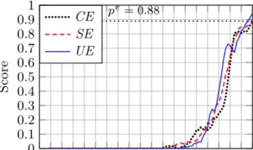
Another way to show the similarity of the results is to plot them. For this we took an aggregate, minus outliers, of all scores and ordered the images from most to least recognizable. Then we plotted the scores from the different environments over this domain. The result can be seen in Figure 7, the plot was smoothed with a window size 5 average function to suppress an extremely jagged appearance due to miss clicks by observers. The recognition rate (RR) is the relative error over all observers per image, an error is coded as 1 so a RR of 0 means all observers recognized the image.
All experimental setups show a very similar curve and the choice of environment does not seem to influence the results. All
0 0.1 0.2 0.3 0.4 0.5 0.6 0.7 0.8 0.9 1 pr= 0.8 ˙8 Score CE SE UE
Fig. 7. Plot of individual scores, per environment, compared to the overall ordering based on an aggregate over all environments.
versions show a gradient from recognizable to unrecognizable
and are trending towards the probability of random choice (pr).
Scaling and the Uncontrolled Environment: The web application (UE) reported back the actual space used for the browser window which was used to display the images. Only one observer used a resolution of 1440p which meant an un-scaled version of the images, the rest (40) used displays of various (smaller) sizes.
From the reported resolutions we reconstruct the follow-ing display sizes which were used (count in parenthesis): 2560x1440p (1), 1920x1200 (8), 1920x1080 (15), 1680x1050 (1), 1600x900 (3), 1400x900 (1), 1366x900 (6), 1280x1024 (1), 1280x768 (3), unknown (2). The unknown resolution were probably from non-maximized browser windows so the actual resolution could not be determined, however the resolution is too small to display the 3×2 array of images without scaling.
IV. Conclusion
The following recommendations and remarks can be made for the acquisition of the recognition threshold from observers. The Match2 protocol is recommended since it gives a higher error rate, allowing for a better differentiation between image recognition than the other proposed protocols. As a side note: a higher number of displayed images, i.e., more than the 6 recommended in Match2, might generate an even better result in terms of error rate but would require the images to be smaller (less detail visible) and increase viewing time to properly assess the images (allowing for fewer images per session).
For the setup we found relatively little difference between the tested environments. The UE setup in theory is fine, but unlimited viewing time potentially leads to viewer fatigue after fewer images, as the time per images can be longer. It should be noted that the viewing time did not have an impact on the results. A shorter viewing time allows for a larger number of comparisons before viewer fatigue sets in, which would suggest a semi-controlled environment, however the uncontrolled en-vironment allows for parallel acquisition and allows to reach a wider number of observers. The controlled environment did not generate any real benefits and is therefore not suggested.
During our tests a short pre-test was run to show the partic-ipants the range of image quality to expect and to familiarize them to the use of the interface. It is suggested to extend this test period to familiarize the observers with the distortion types. A familiarity with the distortion types generates a more consistent behaviour and less outliers as can be seen from the SE vs. CE outlier numbers from bodies consisting almost entirely of computer scientists and medical doctors respectively. For outlier detection hierarchical clustering methods are
rec-ommended as proposed in opposition to direct error measures (MSE).
Acknowledgments
This work was partially supported by the Austrian Science Fund, project no. P27776.
References
[1] C. Bergeron and C. Lamy-Bergor, “Compliant selective encryption for H.264/AVC video streams,” in Proceedings
of the IEEE Workshop on Multimedia Signal Processing, MMSP’05, 2005, pp. 1–4.
[2] S. Jenisch and A. Uhl, “A detailed evaluation of format-compliant encryption methods for JPEG XR-compressed images,” EURASIP Journal on Information Security, vol. 2014, no. 6, 2014.
[3] T. Stütz and A. Uhl, “On efficient transparent JPEG2000 encryption,” in Proceedings of ACM Multimedia and
Secu-rity Workshop, MM-SEC ’07, 2007, pp. 97–108.
[4] H. Hofbauer, A. Uhl, and A. Unterweger, “Transparent Encryption for HEVC Using Bit-Stream-Based Selective Coefficient Sign Encryption,” in 2014 IEEE International
Conference on Acoustics, Speech and Signal Processing (ICASSP). IEEE, 2014, pp. 1986–1990.
[5] H. Hofbauer and A. Uhl, “Identifying deficits of visual security metrics for images,” Signal Processing: Image
Communication, vol. 46, pp. 60 – 75, 2016.
[6] ITU-R BT.2022, “General viewing conditions for subjec-tive assessment of quality of SDTV and HDTV television pictures on flat panel displays BT Series Broadcasting service,” Intl. Telecom. Union, Tech. Rep., 2012.
[7] ITU-R-BT.500-11, “Methodology for the subjective assess-ment of the quality of television pictures,” Intl. Telecom. Union, Tech. Rep., 2004.
[8] G. Cermak, L. Thorpe, and M. Pinson, “Test Plan for Evaluation of Video Quality Models for Use with High Definition TV Content.” Video Quality Experts Group (VQEG)., Tech. Rep., 2009.
[9] IEC-61966-2-1:1999, “Multimedia systems and equipment - Colour measurement and management - Part 2-1: Colour management - Default RGB colour space - sRGB,” Intl. Electrotechnical Commission (IEC), Tech. Rep., 1999. [10] ITU-R BT.500-13, “Methodology for the subjective
asses-ment of the quality of television pictures,” 2012.
[11] N. Ponomarenko, L. Jin, O. Ieremeiev, V. Lukin, K. Egiazarian, J. Astola, B. Vozel, K. Chehdi, M. Carli, F. Battisti, and C.-C. J. Kuo, “Image database TID2013: Peculiarities, results and perspectives,” Signal Processing:
Image Communication, vol. 30, pp. 57–77, 2015.
[12] N. Ponomarenko, O. Ieremeiev, V. Lukin, K. Egiazarian, L. Jin, J. Astola, B. Vozel, K. Chehdi, M. Carli, F. Bat-tisti, and C.-C. J. Kuo, “Color image database TID2013: Peculiarities and preliminary results,” in Proceedings of
4th Europian Workshop on Visual Information Processing (EUVIP’13), 2013, pp. 106–111.
[13] ITU-T REC P.910, “SERIES P: TELEPHONE TRANS-MISSION QUALITY audiovisual quality in multimedia services,” 1996.
[14] ITU-R BT.500-11, “Methodology for the subjective asses-ment of the quality of television pictures,” 2002.