HAL Id: hal-01393364
https://hal.inria.fr/hal-01393364
Submitted on 7 Nov 2016
HAL is a multi-disciplinary open access
archive for the deposit and dissemination of
sci-entific research documents, whether they are
pub-lished or not. The documents may come from
teaching and research institutions in France or
abroad, or from public or private research centers.
L’archive ouverte pluridisciplinaire HAL, est
destinée au dépôt et à la diffusion de documents
scientifiques de niveau recherche, publiés ou non,
émanant des établissements d’enseignement et de
recherche français ou étrangers, des laboratoires
publics ou privés.
Relevance of Context for the Temporal Completion of
Call Detail Record
Guangshuo Chen, Sahar Hoteit, Aline Carneiro Viana, Marco Fiore, Carlos
Sarraute
To cite this version:
Guangshuo Chen, Sahar Hoteit, Aline Carneiro Viana, Marco Fiore, Carlos Sarraute. Relevance of
Context for the Temporal Completion of Call Detail Record. [Research Report] RT-0482, INRIA
Saclay. 2016, pp.14. �hal-01393364�
ISSN 0249-0803 ISRN INRIA/R T --482--FR+ENG
TECHNICAL
REPORT
N° 482
November 2016 Project-Teams INFINERelevance of Context for
the Temporal Completion
of Call Detail Record
Guangshuo Chen, Sahar Hoteit, Aline Carneiro Viana, Marco Fiore,
Carlos Sarraute
RESEARCH CENTRE SACLAY – ÎLE-DE-FRANCE
1 rue Honoré d’Estienne d’Orves Bâtiment Alan Turing
Campus de l’École Polytechnique 91120 Palaiseau
Relevance of Context for the Temporal
Completion of Call Detail Record
Guangshuo Chen
∗†, Sahar Hoteit
‡, Aline Carneiro Viana
†,
Marco Fiore§, Carlos Sarraute
¶Project-Teams INFINE
Technical Report n° 482 — November 2016 — 14 pages
Abstract: Call Detail Records (CDRs) are an important source of information in the study of different aspects of human mobility. However, their utility is often limited by spatio-temporal sparsity. In this paper, we first evaluate the effectiveness of CDRs in measuring relevant mobility features. We then investigate whether the information of user’s instantaneous whereabouts pro-vided by CDRs enables us to estimate positions over longer time spans. Our results confirm that CDRs ensure a good estimation of radii of gyration and important locations, yet they lose some location information. Most importantly, we show that temporal completion of CDRs is straight-forward and efficient: thanks to the fact that they remain fairly static before and after mobile communication activities, the majority of users’ locations over time can be accurately inferred from CDRs. Finally, we observe the importance of user’s context, i.e., of the size of the current network cell, on the quality of the CDR temporal completion.
Key-words: Call detail records, user mobility, human trajectories, important locations, location boundaries
This work was supported by the EU FP7 ERANET program under grant CHIST-ERA-2012 MACACO. ∗Université Paris Saclay, France
†INRIA Saclay, France
‡Ecole d’ingénieurs du numérique ISEP, France §CNR - IEIIT, Italy
Pertinence du contexte pour l’achèvement temporel des
statistiques d’appel
Résumé : Les statistiques d’appel (ou en anglais Call Detail Records - CDR) sont une impor-tante source d’information dans l’étude des différents aspects de la mobilité humaine. Cependant, leur utilité est souvent limitée par son spartiété spatio-temporelle. Dans cet article, nous évalu-ons d’abord l’efficacité de l’utilisation ded CDR pour la mesure des caractéristiques de mobilité pertinentes. Nous nous demandons ensuite si les informations de localisation instantanée de l’utilisateur fournies par les CDR nous permettent d’estimer leurs positions sur des périodes longues. Nos résultats confirment que les CDR assurent une bonne estimation des rayons de giration et des emplacements importants, mais ils perdent certaines informations de localisation. Plus important encore, nous montrons que l’achèvement temporel des CDR est simple et efficace: grâce au fait qu’ils restent relativement statiques avant et après les activités de communication mobile, la majorité des emplacements des utilisateurs dans le temps peut être correctement dé-duite des CDR. Enfin, on observe l’importance du contexte de l’utilisateur, c’est-à-dire de la taille de la cellule de réseau actuelle, sur la qualité de l’achèvement temporel des CDR.
Mots-clés : Statistiques d’appel; Mobilité des utilisateurs; Trajectoires humaines; Endroits importants; bordures de localisation
Relevance of Context for the Temporal Completion of Call Detail Record 3
1
Introduction
The urbanization worldwide is bringing a variety of challenges to city development and sustain-ability, and telecommunications networks are no exception. To manage the complexity of the smart urban environment of tomorrow, the understanding of human mobility patterns become es-sential. A variety of network-related operations, such as paging in cellular networks [1], location-based recommender systems [2], mobile service traffic dynamics [3], cache performance [4], al-ready leverage interesting insights from human mobility patterns. These studies strongly rely on spatio-temporal datasets describing human mobility. Call Detail Records (CDRs) are the primary source of data for large-scale studies on urban populations of millions of users [5].
CDRs contain information about when, where and how a mobile phone subscriber gener-ates voice calls and text messages, and are collected by mobile network operators for billing purposes [5]. Owing to the bursty and irregular nature of the communication activities they capture, CDRs are usually are sparse in time [6]. Hence, when considering CDR datasets as a source of information on human mobility, significant challenges arise about (i) whether and to what extent does the sparsity of CDRs affect mobility studies, and (ii) if it is possible to solve the sparsity problem by completing CDR data over time.
We address these problems in two ways: Firstly, we evaluate how CDRs are biased in measur-ing mobility features such as evaluatmeasur-ing the radius of gyration, countmeasur-ing user’s entire locations, and identifying user’s important locations. Secondly, we study whether leveraging the infor-mation of user’s instantaneous whereabouts provided by CDRs is capable of locating the user continuously in time.
Our work relates to the topic of measuring possible biases when using CDR datasets. A seminal work in this sense was performed by Ranjan et al. [7], who showed that CDRs are capable of identifying important locations, and exposed the bias of working only on very active CDR users as they may not represent the entire population. Besides, [8] showed that using CDR positioning information may lead to a distance error within 1 km compared with ground-truth collected by five voluntaries. These observations were later confirmed in [9], using a GPS-referenced dataset containing 84 users. Our results confirm the observations in [7] while using datasets of tens of thousands of users, hence much larger than that employed in [9]. Relevant to our study are also works on CDR data completion. The legacy approach is assuming that the user remains static from some time before and after each communication activity. The span of the static period, named location boundary hereinafter, is a system parameter that is fixed and hardly validated [10, 9]. Our results extend previous analyses, showing that user’s context shall be taken into account to set the value of the location boundary parameter dynamically.
Our contributions are summarized as follows:
• Our investigation is based on the mobility dataset described in Sec. 2. The geo-referenced data captures the location of tens of thousands of users at every 5 minutes on average and allows scaling the CDR bias and completion analysis at unprecedented levels.
• We evaluate the possible limitations brought by the sparsity of CDRs, to measure human mobility features. We confirm –at such larger scale– findings on the quality and limitations of CDRs in measuring human mobility, in Sec. 3.
• We evaluate the impact of location boundaries on the spatial error of completed CDR data and show how the cell coverage affects the results. Details are provided In Sec. 4.
• Overall, our results highlight the importance of adaptive location boundaries, and provide insights on the design of such an approach, as summarized in Sec. 5.
4 Chen & Hoteit & Viana & Fiore & Sarraute
2
Dataset
We use in our study two datasets collected by a major cellular network operator in Mexico. The data cover the [10am, 6pm] time interval, prevailing working hours, during two non-consecutive days, as shown in Table. 1. Both datasets allow the study of human mobility but at different granularity: the first describes fine-grained mobility while the second provides coarse-grained information.
• Fine-grained dataset is composed of Internet data records, called hereafter flows. These are obtained every time a mobile device establishes a TCP/UDP session for some services (e.g., Facebook, Google, WhatsApp, P2P). Each flow entry contains the hashed device identifier, the type of service, the volume of exchanged upload and download data (in KB), the timestamps denoting the start and end times of the session, and more importantly, the cell tower location where the session has ended.
• Coarse-grained dataset is obtained through Call Detail Records. Each CDR entry pro-vides the detailed information of an event (i.e., initiating or receiving a phone call, sending or receiving an SMS or MMS). It consists of the event duration, the hashed identifiers of the involved devices in the considered event (i.e., caller/callee in a phone call, and sender/receiver in an SMS or MMS), and the cell tower location of the beginning of the event.
2.1
Dataset filtering
To tackle the undesirable effects of the widely encountered phenomenon of cell-tower oscilla-tion1 [11], we apply the recursive look-ahead filter proposed in [12] on both datasets.
Never-theless, as the CDR dataset is already very sparse in time, upon detection of the oscillation phenomenon, instead of removing the corresponding log, we modify its location to that of the closest log (in time) in the fine-grained dataset (this closet log is within 5 minutes on average). By doing this, we preserve the original granularity of the CDR dataset, while ensuring positioning data correctness.
Furthermore, to guarantee that the fine-grained dataset (flow dataset) has a considerable temporal granularity, we filter out the subscribers having an inter-event time (i.e., the time between two consecutive flows) higher than 20 minutes. This filtered data serves for the rest of the paper as the ground-truth dataset. The statistical distribution of the per-user inter-event time is shown in Fig. 1(a). We note that in 98% of cases, the inter-event time is less than 5 minutes, and in less than 1% of cases, the inter-event time is higher than 10 minutes.
We also plot in Fig. 1(b) the CDF of the number of flows per user (as solid lines) for com-parison, which clearly tells that the fine-grained dataset brings richer information about users’ movement because the number of flows is far more than of CDRs in the coarse-grained dataset. High temporal granularity supports the use of trajectories in the fine-grained dataset as the ground truth in our analysis.
2.2
Day distinction
Throughout our study, we evaluate separately the results for the two days of data. As Sundays and Mondays are known to yield substantial differences regarding users’ communication activity and mobility, our approach let us observe how such differences affect our specific problem. The
1Cell-tower oscillations occur when the association of a static user to the mobile network swings among multiple cell towers, e.g., due to load balancing or fluctuations in the RF environment.
Relevance of Context for the Temporal Completion of Call Detail Record 5 Table 1: Dataset
Date(s) Users Rare CDR users CDR usersFrequent Sunday July 19, 2015 10, 856 6, 154 4, 702 Monday July 20, 2015 14, 353 7, 215 7, 138
(a)
100 101 102 103 104 105
Number of records (flows or CDRs) per user 0.0 0.2 0.4 0.6 0.8 1.0 F (x ) CDF Flows: Sunday Flows: Monday CDRs: Sunday CDRs: Monday (b)
Figure 1: (a) CDF of the inter-event time in the ground-truth dataset; (b) CDF of the number of records (flows or CDRs) per user in a weekend and a weekday.
number of users appearing in each day and dataset is reported in Tab. 1. We plot in Fig. 1(b) the cumulative distribution function (CDF) of the number of calls and flows per user on Sunday and Monday. Focusing on calls, 35% of users on Sundays and 20% on Monday have only one call during the observed period, and 3% of users have more than 10 phone calls on Sunday while this percentage increases to 7% on Monday. These results are aligned with previous findings, as users tend to be more active during working days.
2.3
Users categories
We separate the users in the CDR dataset into two different categories:
• Rare CDR users are users who are not very active in making or receiving voice calls, and sending or receiving SMS/MMS. As in [13], we use the threshold of 0.5 CDR/hour below which the user is considered to belong to this category.
• Frequent CDR users are those who are comparatively active. They have more than 0.5CDR/hour.
The number of users in each category is shown in Table 1. We notice that 49% of the users on Monday and 43% on Sunday belong to the frequent CDR user category.
In the rest of the paper, we focus on the use of the filtered coarse-grained dataset for the study of human mobility. We compare the results with those obtained from the filtered fine-grained dataset, which represents our ground truth. During our whole analysis, we account for day and users category diversity.
6 Chen & Hoteit & Viana & Fiore & Sarraute
3
CDRs for human mobility studies
To validate the accuracy and correctness of CDR-based human mobility studies, we make a comparative study between the coarse-grained and the ground-truth datasets as a function of different criteria that are widely used to assess human mobility analysis. In particular, we consider two criteria, i.e., the span of movement and the per-user important locations.
3.1
Span of human movement
The first study consists of examining whether CDRs can be adapted for measuring the geograph-ical span of movement of subscribers. For that, we consider the radius of gyration parameter, computed for each user u ∈ U, where U is the observed population. It is defined as the deviation of user’s positions to its centroid position, as follows:
Rug = v u u t 1 n n X i=1 (ru i − r u centroid), (1) where ru
centroidis the center of mass of user’s u locations in the observation period, i.e., r u centroid= 1 n Pn i=1r u
i. This parameter has been widely used for studying different aspects of human
mobil-ity [3, 13, 14, 15].
In our study, we compute, for each user u, his radius of gyration Ru
g using the coarse-grained
and the ground-truth datasets, for different categories of users (i.e., all users, rare CDR users, and
0 2 4 6 8 10
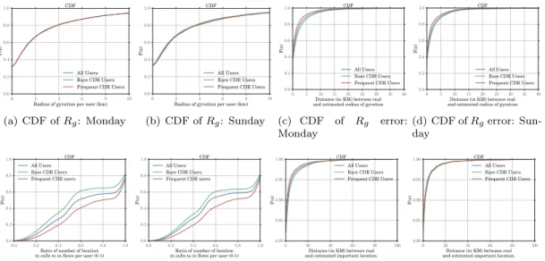
Radius of gyration per user (km) 0.0 0.2 0.4 0.6 0.8 1.0 F(x) CDF All Users Rare CDR Users Frequent CDR Users (a) CDF of Rg: Monday 0 2 4 6 8 10
Radius of gyration per user (km) 0.0 0.2 0.4 0.6 0.8 1.0 F(x) CDF All Users Rare CDR Users Frequent CDR Users (b) CDF of Rg: Sunday 0 5 10 15 20 25 30 35 40
Distance (in KM) between real and estimated radius of gyration 0.0 0.2 0.4 0.6 0.8 1.0 F(x) CDF All Users Rare CDR Users Frequent CDR Users (c) CDF of Rg error: Monday 0 5 10 15 20 25 30 35 40
Distance (in KM) between real and estimated radius of gyration 0.0 0.2 0.4 0.6 0.8 1.0 F(x) CDF All Users Rare CDR Users Frequent CDR Users (d) CDF of Rgerror: Sun-day 0.0 0.2 0.4 0.6 0.8 1.0
Ratio of number of location in calls to in flows per user (0-1) 0.0 0.2 0.4 0.6 0.8 1.0 F(x) CDF All Users Rare CDR Users Frequent CDR users (e) CDF of rNL: Monday 0.0 0.2 0.4 0.6 0.8 1.0
Ratio of number of location in calls to in flows per user (0-1) 0.0 0.2 0.4 0.6 0.8 1.0 F(x) CDF All Users Rare CDR Users Frequent CDR users (f) CDF of rNL: Sunday 0 20 40 60 80 100
Distance (in KM) between real and estimated important location. 0.80 0.85 0.90 0.95 1.00 F(x) CDF All Users Rare CDR Users Frequent CDR Users (g) CDF of ∆D: Monday 0 20 40 60 80 100
Distance (in KM) between real and estimated important location. 0.80 0.85 0.90 0.95 1.00 F(x) CDF All Users Rare CDR Users Frequent CDR Users (h) CDF of ∆D: Sunday
Figure 2: (a)(b) CDF of the radius of gyration over the observed population on (a) Monday and (b) Sunday; (c)(d) CDF of the distance between each user’s Rg estimated by the fine-grained
trajectory and Rgby the coarse-grained trajectory on (c) Monday and (d) Sunday; (e)(f) CDF of
the radio rNLof the number of location in each user’s coarse-grained trajectory to the one in her
fine-grained trajectory on (e) Monday and (f) Sunday; (g)(h) CDF of the distance between each user’s real and estimated important locations located by her fine- and coarse-gained trajectories on (g) Monday and (f) Sunday.
Relevance of Context for the Temporal Completion of Call Detail Record 7 frequent CDR users). The obtained values represent the estimated (due to the spatial sparsity of the dataset) and the real radius of gyration, respectively.
The results are depicted in Fig. 2, where Fig. 2(a)(c)(e) represent those obtained from the weekday (Monday, July 20,2015 in our case) and Fig. 2(b)(d)(f) during the weekend (Sunday, July 29, 2015). We can clearly note that:
• There is no much difference between weekends and weekdays in terms of radius of gyration. • For the three different categories of users (i.e., all users, rare CDR users, and frequent CDR users), the radius of gyration shows almost the same distribution, as shown in Fig. 2(a)(b). It indicates that one can get a reliable distribution of Rg from a certain number of users
even if their interaction frequency with the cellular network is not very high.
• For approximately 90% of all the considered users, the error (distance in Km) between the real and the estimated radii of gyration is less than 5 km, as in Fig. 2(c) and 2(d). • Intuitively, a more accurate Rgcan be obtained by taking into consideration more locations
visited by the user. This statement is validated indeed in Fig. 2(c): we notice that 92% of frequent CDR users have an error lower than 5 km, while the percentage decreases to 86% for rare CDR users. The same observation holds for the weekends as shown in Fig. 2(d). Note that this error is estimated based on cell tower locations. When leveraging more precise GPS data, only 26% of users have an error larger than ±1 km [9].
• Due to the spatio-temporal sparsity of CDRs, the mobility information in CDR-based studies is usually incomplete. For this, we study in Fig. 2(e) and Fig. 2(f) the ratio rNL
between the total number of unique locations detected from CDRs (NCDR
L ) and from the
ground-truth (NFlow L ): rNL= N CDR L /N Flow L . (2)
We notice that, on Monday, 42% of the observed population (i.e., all users) have their rNL
higher than 80%, i.e., only 20% of the unique locations visited by the users do not appear in the CDR dataset. However, the percentage of users having this criterion is slightly higher for the frequent CDR users (around 50%), but it is lower for the rare CDR users (37%). These results confirm the benefits of using frequent CDR dataset to ensure a better completeness of user’s locations. We note that the same results hold for weekends.
3.2
Important locations
An important step in characterizing human mobility consists of identifying user’s important locations. As users have usually repetitive daily routines, a common and simple solution to identify these locations consists in (i) separating the whole day period into two major sub-periods (e.g., daytime and nighttime), and (ii) determining the most frequent location in each sub-period. As our datasets cover only the period between [10am, 6pm], we infer a user’s work location by the cell where the user spends most of her daytime.
To check the accuracy of CDRs-based studies in determining important locations, we com-pute for each user her important locations using both the coarse-grained and the ground-truth datasets. In detail, the estimated and the real important locations are respectively located as the one where the most CDRs are observed and the one where the user spends the most time. Then, we compute the distance between these two important locations as ∆D. We infer users’ work location using the weekday data, while the data from the weekends permit to infer the most visited locations during weekends.
8 Chen & Hoteit & Viana & Fiore & Sarraute Fig. 2(g) and Fig. 2(h) show the cumulative distribution function of the distance between the real and the estimated important locations in Km and on the weekday and weekend, respectively. We observe the following:
• The error between the real and the estimated important locations is null for approximately 85%of all the users, indicating that the usage of the coarse-grained dataset is fairly sufficient for inferring these important locations.
• For the rest of users (15% of the total users), the error between real and estimated important locations is non-null: we have around 10% of the users with a relatively small error (∆D < 5 km) while 5% of the users have an error higher than 5 km.
• There is no difference in the distribution of ∆D between rare CDR and frequent CDR users, except a slight difference on Monday as shown in Fig. 2(g). The reason behind that can be interpreted by the fact that people are usually more active in the cellular network on weekdays (as shown in Fig. 1(b)) and hence, generate more phone calls/messages from the corresponding important locations.
4
CDR completion via location boundaries
The results in Sec. 3 evidence the quality of mobility information that can be inferred from CDR data, regarding span of user’s movement and important locations. They also indicate that some bias is present: specifically, by relying on CDRs, one cannot hope to capture the entire set of user’s locations, as transient and less important places visited by users are lost. The good news is that, even in those cases, the error introduced by CDRs is relatively small. Overall, the observations above motivate the use of CDR datasets, which are much easier to obtain than fine-grained flow data [5], for the analysis of human mobility.
However, a major limitation of CDRs remains their temporal sparsity. Indeed, CDR only provides instantaneous information about the location of users at a few time instants over a whole day. CDR temporal completion aims at solving this problem, by extending the time span of the position associated with each communication activity to some location boundary. In other words, one assumes that users remain static, or at least do not move beyond coverage of the same cell, for a time corresponding to a location boundary before and after a communication activity takes place.
In this section, we provide two contributions to the problem of CDR completion. First, we assess how the parametrization of location boundaries affects the quality of the completed data. Second, we investigate the existence of correlations between such completed CDR quality and a user’s context, defined as the coverage of his associated cell.
4.1
Complementing the ground-truth dataset
Two preliminary steps are needed for our analysis, and are discussed next. 4.1.1 Filling temporal gaps in the fine-grained dataset
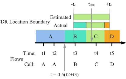
As previously mentioned, the fine-grained dataset presented in Sec. 2 serves as our ground truth. However, also this dataset is discrete over time, and so are the locations of users it records. To reconstruct a continuous dataset, we have to fill the temporal gaps between users’ locations. To this end, we apply the simple approach depicted in Fig. 3. For each consecutive pairs of user’s locations (ti, ci)and (ti+1, ci+1), where tiand cicorresponds respectively to the time instant and
cell location of ith log of the user, we proceed as follows.
Relevance of Context for the Temporal Completion of Call Detail Record 9
Time:
Cell:
t2
t3
t4
t5
t1
A
A
B
C
D
A
B
C
D
t = 0.5(t2+t3)
Flows
t
CDR+t
d-t
dActual
Estimated
CDR Location Boundary
Figure 3: A demo of (1) complementing the fine-grained trajectory and (2) the CDR location boundary: (1) Suppose five consecutive flows at time t1, . . . , t5 at cell A, B, C, D. Flows t1, t2 are merged together as they are observed continuously at the same cell A. The handover time from the cell A to B is set at the mid time of t2 and t3. (2) A fixed-period location boundary (tCDR− td, tCDR+ td)is given attached with a CDR at time tCDR at the cell C. In this location
boundary, the user is assumed to be at the cell C while actually she moves from the cell B to D, which causes a spatial error.
1. The user remains attached to the same cell ci in the interval of time [ti, ti+1]if ci= ci+1.
2. The user is attached to cell ci during [ti, t (i,i+1)
HO ] and to cell ci+1 during [t (i,i+1)
HO , ti+1], if
ci6= ci+1. The parameter t (i,i+1)
HO is defined as the handover time instant from cell cito cell
ci+1. For simplicity, we consider that the handover time instant between two cells is the
middle of the interval [ti, ti+1].
4.1.2 Estimating cell coverage
In addition to visited location information from both coarse and fine-grained datasets, we in-formation about cell tower deployment, consisting of 14, 953 cell tower locations2 that cover the
whole Mexico.
We estimate cell coverage by computing a Voronoi tessellation [16]: this is an unavoidable choice since we do not have information about the transmit power of each cell tower or RF propagation environment, and we have to assume an homogeneous propagation environment and an isotropic radiation of power in all directions at each cell tower. To account for the fact that real-world deployments result in overlapping coverage, we then define the cell coverage as the smallest circle centered at the cell tower location and whose radius is the largest distance between such location and the Voronoi polygon contour. The resulting circle covers entirely the Voronoi polygon, and yields overlapping coverage at cell boundaries. We find that 70% of cells have a radius < 3 km, with a median radius of 1 km.
2Cell tower locations were provided by the operator (52%) or third-party services (48%, obtained via Google, Mozilla, or OpenCellID services).
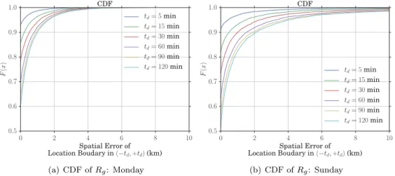
10 Chen & Hoteit & Viana & Fiore & Sarraute 0 2 4 6 8 10 Spatial Error of Location Boudary in (−td, +td)(km) 0.5 0.6 0.7 0.8 0.9 1.0 F (x ) CDF td= 5min td= 15min td= 30min td= 60min td= 90min td= 120min (a) CDF of Rg: Monday 0 2 4 6 8 10 Spatial Error of Location Boudary in (−td, +td)(km) 0.5 0.6 0.7 0.8 0.9 1.0 F (x ) CDF td= 5min td= 15min td= 30min td= 60min td= 90min td= 120min (b) CDF of Rg: Sunday
Figure 4: CDF of the spatial error of the location boundary over the observed population grouped by time period on (a) Monday and (b) Sunday.
4.2
Errors of fixed-period location boundaries
Here, we evaluate the fixed-period location boundaries in terms of spatial error. Suppose that a CDR entry is recorded at time tCDR at cell cCDR. Completing the CDR entry with a location
boundary of timespan td means that the user is assumed to be within the cell cCDR during the
time interval [tCDR− td, tCDR+ td]. An example is shown in Fig. 3.
Intuitively, an error may occur if the user moves to other cells during this time interval. We define the spatial error as the average cumulative distance error, as follows:
err =
RtCDR+td
tCDR−td kcCDR− crealkdistdt
2td
. (3)
This measure represents the average distance between a user’s real cell location creal and the
estimated cell location cCDR during [tCDR− td, tCDR+ td]. For each user, we measure the spatial
error using the corresponding CDR logs in the observation period. The interpretation of this spatial error is straightforward:
• When a location boundary has an err = 0, it means that during its time period the user stays at the cell cCDR at all time, and the estimation of td may be conservative: a large td
could be more adapted in this case.
• When having an err > 0, it means that the location boundary is over-sized: the user actually moves to other cells in its time period and thus, a smaller td should be more
adapted.
We plot in Fig. 4 the CDF of the spatial error over all location boundaries identified from CDRs. As we expected, we observe that 95% of CDRs on Monday (cf. 92% on Sunday) have err = 0 location boundaries of (−150, 150)and 60% on Monday (cf. 53% on Sunday) even have
ones of (−1200, 1200), which strongly supports the fact that the users remain in the cell coverage
temporally around their CDR activities. However, note that on Monday approximately 35% (cf. 40% on Sunday) of the observed users are stable, i.e., each of them has only one location observed in her fine-grained trajectory and consequently, Rg = 0. The high percent of location
Relevance of Context for the Temporal Completion of Call Detail Record 11 boundaries with err = 0 shown in Fig. 4 may credit to these users because any tdin their location
boundaries will be conservative: no spatial error occurs at all. To further analyze the spatial error, we exclude these users from the next evaluation, where only mobile (Rg > 0) users are involved.
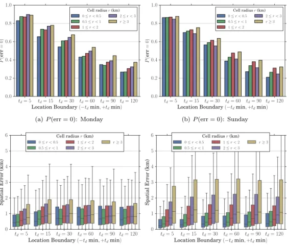
Let us first evaluate the probability of having a null location boundary error, i.e., Pr(err = 0). Fig. 5(a) and Fig. 5(b) present the probability of having a null spatial error, i.e., P (err = 0), when applying a location boundary with td= 5/15/30/60/90/120minutes respectively on Monday and
Sunday, grouped by the cell radius. We note the following.
• The probability P (err = 0) decreases with the increasing period marked by td, indicating
that using a large time period on the location boundary decreases the probability of null spatial error. For instance, for td = 150, the probability of having a non-null spatial error
td= 5 td= 15 td= 30 td= 60 td= 90 td= 120
Location Boundary (−tdmin, +tdmin)
0.0 0.2 0.4 0.6 0.8 1.0 P (err = 0) Cell radius r (km) 0≤ r < 0.5 0.5≤ r < 1 1≤ r < 2 2≤ r < 3 r≥ 3
(a) P (err = 0): Monday
td= 5 td= 15 td= 30 td= 60 td= 90 td= 120
Location Boundary (−tdmin, +tdmin)
0.0 0.2 0.4 0.6 0.8 1.0 P (err = 0) Cell radius r (km) 0≤ r < 0.5 0.5≤ r < 1 1≤ r < 2 2≤ r < 3 r≥ 3 (b) P (err = 0): Sunday td= 5 td= 15 td= 30 td= 60 td= 90 td= 120
Location Boundary (−tdmin, +tdmin)
0 1 2 3 4 5 6 Spatial Error (km) Cell radius r (km) 0≤ r < 0.5 0.5≤ r < 1 1≤ r < 2 2≤ r < 3 r≥ 3 (c) Error: Monday td= 5 td= 15 td= 30 td= 60 td= 90 td= 120
Location Boundary (−tdmin, +tdmin)
0 1 2 3 4 5 6 Spatial Error (km) Cell radius r (km) 0≤ r < 0.5 0.5≤ r < 1 1≤ r < 2 2≤ r < 3 r≥ 3 (d) Error: Sunday
Figure 5: Spatial error of the fixed-period location boundary for the users with their Rg >
0: (a)(b) the probability to have an err = 0 location boundary (−td, td) where td is
5/15/30/60/90/120 minutes under the certain groups of the cell radius on (a) Monday and (b) Sunday; (c)(d) Boxplot of the spatial error grouped by the cell radius and the time period of location boundary on (c) Monday and (d) Sunday. Each box denotes the median and 25th
− 75th
percentiles and the whiskers denote 5th
− 95thpercentiles.
12 Chen & Hoteit & Viana & Fiore & Sarraute varies between 22% to 35% depending on the date and on the cell radius. However, when a larger tdis used, the probability significantly increases (e.g., for td= 300, the probability
of non-null spatial error grows from 35% to 50%).
• The probability P (err = 0) increases positively with the cell radius r. This trend is clearly seen on both Monday and Sunday (except for 2 < r < 3 km cell radius), indicating that the cell size has an impact on the time interval during which the user stays within the cell coverage. Intuitively, when the user is moving, a handover may happen quite often if the user’s current cell is small; however, if the user is attached to a cell tower having a big area coverage, the probability of handover decreases.
Overall, we can say that there is a strong correlation between the location boundary and the cell coverage. However, since the CDR logs of a user are usually sparse in time, using a small fix-period location boundary could only cover an insignificant amount of time, while using a big location boundary increases the risk of having a non-null spatial error. To investigate this trade-off, we plot the variation of the statistical distribution of the spatial errors after excluding the null errors (i.e., keeping only err > 0) in Fig. 5(c) and Fig. 5(d).
• The spatial error varies widely, it goes from less than 1 km to very huge values (up to 8 km). For such high errors, the fixed-period location boundary is thus unsuitable especially with high users’ movement patterns.
• Under the same values of td and r, larger differences emerge between Monday and Sunday,
which confirms previous findings that users move more on weekdays.
• The spatial error grows with the cell radius: when the cell size increases, the variation of the error becomes wider and the mean value also increases. This is reasonable because the higher the cell radius is, the farther the cell is from its neighbors. Hence, when a spatial error occurs, it means that the user is actually in a far cell that has a larger distance to cCDR.
Overall, we can say that location boundary could estimate users’ locations with a high ac-curacy when td is small. That validates previous findings that state that users usually stay
in proximity of call locations for a while. However, the accuracy is significantly reduced when increasing the location boundary, up to the point where using fixed-period location boundaries causes large spatial errors. Hence, the trade-off between the time coverage and the accuracy should be carefully considered when using location boundaries.
5
Discussion and conclusion
Thus far, we have shown the capability of using location boundaries of identifying users’ locations. Since the accuracy is related to the context such as the cell coverage, apparently using a fixed time period is insufficient for the location boundary: we see that sometimes it makes a large spatial error. Hence when using CDRs, an adaptive approach to determine the time period is necessary. Here we present some guidelines for the design of such an approach.
Firstly, consider identifying stable users. Though it is a challenging task due to the high sparsity of CDR logs, identifying such type of users in CDRs is feasible over a short time period, e.g., one during which CDRs are captured in high frequency. Secondly, determine the time period regarding cell coverage. A big cell has a high tolerance to errors as we observed in Sec. 4. Intuitively, a large time period should be assigned when the user is located at a big cell.
Relevance of Context for the Temporal Completion of Call Detail Record 13 In conclusion, we identify the key challenges of CDRs-based human mobility analysis regard-ing accuracy and correctness in this paper. Our results validate previous findregard-ings of the limits of CDRs. Moreover, we evaluate the accuracy of CDR-based location boundaries regarding spatial error. We find that with a particular time period, the fixed-period location boundary could have an accurate estimation of user’s cell tower location around the activities captured by CDRs while it may cause a huge error. In future, we will work on the design of an adaptive approach along the guidelines above.
References
[1] H. Zang and J. C. Bolot, “Mining call and mobility data to improve paging efficiency in cellular networks,” in MobiCom ’07: Proceedings of the 13th annual ACM international conference on Mobile computing and networking. New York, New York, USA: ACM, Sep. 2007, pp. 123–134.
[2] Y. Zheng, L. Zhang, X. Xie, and W.-Y. Ma, “Mining interesting locations and travel se-quences from gps trajectories,” in Proceedings of the 18th international conference on World wide web. ACM, 2009, pp. 791–800.
[3] U. Paul, A. P. Subramanian, M. M. Buddhikot, and S. R. Das, “Understanding traffic dynamics in cellular data networks,” in INFOCOM, 2011 Proceedings IEEE. IEEE, 2011, pp. 882–890.
[4] K. Y. Lai, Z. Tari, and P. Bertok, “Supporting user mobility through cache relocation,” Mobile Information Systems, vol. 1, no. 4, pp. 275–307, 2005.
[5] D. Naboulsi, M. Fiore, S. Ribot, and R. Stanica, “Large-scale Mobile Traffic Analysis: a Survey,” IEEE Communications Surveys & Tutorials, vol. PP, no. 99, pp. 1–1, 2015. [6] A.-L. Barabasi, “The origin of bursts and heavy tails in human dynamics,” Nature, vol. 435,
no. 7039, pp. 207–211, 2005.
[7] G. Ranjan, H. Zang, Z.-L. Zhang, and J. Bolot, “Are call detail records biased for sampling human mobility?” ACM SIGMOBILE Mobile Computing and Communications Review, vol. 16, no. 3, pp. 33–44, 2012.
[8] S. Isaacman, R. Becker, R. Cáceres, S. Kobourov, M. Martonosi, J. Rowland, and A. Var-shavsky, “Ranges of human mobility in los angeles and new york,” in Pervasive Computing and Communications Workshops (PERCOM Workshops), 2011 IEEE International Confer-ence on. IEEE, 2011, pp. 88–93.
[9] S. Hoteit, G. Chen, A. Viana, and M. Fiore, “Filling the gaps: On the completion of sparse call detail records for mobility analysis,” in ACM Chants, 2016.
[10] H. H. Jo, M. Karsai, J. Karikoski, and K. Kaski, “Spatiotemporal correlations of handset-based service usages,” EPJ Data Science, vol. 1, pp. 1–18, 2012.
[11] M. A. Bayir, M. Demirbas, and N. Eagle, “Mobility profiler: A framework for discovering mobility profiles of cell phone users,” Pervasive and Mobile Computing, vol. 6, no. 4, pp. 435–454, 2010.
14 Chen & Hoteit & Viana & Fiore & Sarraute [12] C. Horn, S. Klampfl, M. Cik, and T. Reiter, “Detecting outliers in cell phone data: correcting trajectories to improve traffic modeling,” Transportation Research Record: Journal of the Transportation Research Board, no. 2405, pp. 49–56, 2014.
[13] C. Song, Z. Qu, N. Blumm, and A.-L. Barabási, “Limits of Predictability in Human Mobil-ity,” Science, vol. 327, no. 5968, pp. 1018–1021, Feb. 2010.
[14] M. C. González, C. A. Hidalgo, and A.-L. Barabási, “Understanding individual human mobility patterns,” Nature, vol. 453, no. 7196, pp. 779–782, Jun. 2008.
[15] S. Hoteit, S. Secci, S. Sobolevsky, C. Ratti, and G. Pujolle, “Estimating human trajectories and hotspots through mobile phone data,” Computer Networks, vol. 64, pp. 296–307, 2014. [16] J. Portela and M. Alencar, “Cellular network as a multiplicatively weighted voronoi dia-gram,” in CCNC 2006. 2006 3rd IEEE Consumer Communications and Networking Con-ference, 2006., vol. 2. IEEE, 2006, pp. 913–917.
RESEARCH CENTRE SACLAY – ÎLE-DE-FRANCE
1 rue Honoré d’Estienne d’Orves Bâtiment Alan Turing
Campus de l’École Polytechnique 91120 Palaiseau
Publisher Inria
Domaine de Voluceau - Rocquencourt BP 105 - 78153 Le Chesnay Cedex inria.fr