Calibration of Mesoscopic Traffic Simulation
Models for Dynamic Traffic Assignmen
MASACHTTSiu STITUE
by
OF TECHNOLOGYKunal Kamlakar Kund6
SEP 1 9 ('J02
B.Tech. in Civil Engineering (2000) LIBRARIEsIndian Institute of Technology, Bombay, India
Submitted to the Department of Civil and Environmental Engineering
in partial fulfillment of the requirements for the degree of PARKECR Master of Science in Transportation
at the
MASSACHUSETTS INSTITUTE OF TECHNOLOGY September 2002
@
Massachusetts Institute of Technology 2002. All rights reserved.A u th or ... ,. . ...
Department ofCivil and Environmental Engiering August 9, 2002
Certified by... ...
Moshe E. Ben-Akiva Edmund K.Turner Professor Department of Civil and Environmental Engineering Thesis Supervisor
Certified by... , ... ..
Haris N. Koutsopoulos Operations Research Analyst Volpe Nationj Transportation Systems Center Thesis Supervisor
Accepted bj ...
Oral Buyukozturk Chairman, Department Committee on Graduate Students
Calibration of Mesoscopic Traffic Simulation Models for
Dynamic Traffic Assignment
by
Kunal Kamlakar Kunde
B.Tech. in Civil Engineering (2000) Indian Institute of Technology, Bombay, IndiaSubmitted to the Department of Civil and Environmental Engineering on August 9, 2002, in partial fulfillment of the
requirements for the degree of Master of Science in Transportation
Abstract
This thesis tackles the calibration of mesoscopic flow propagation models in the traffic dynamics simulator of the DynaMIT Dynamic Traffic Assignment system. A three-stage methodology is developed to carry out calibration in a sequential manner at increasing levels of aggregation. Two stochastic optimization approaches - one based on stochastic gradient approximation and one that does not employ gradients - are applied to carry out the calibration along the lines of a simulation optimization prob-lem. The parameters to be calibrated are the umin, uf, ko, kjam, o', and / parameters in the speed-density relationship for every road segment and the capacities of all road segments and intersections. The methodology is applied to a study network extracted from the Orange County region in California using traffic surveillance data obtained from the California Department of Transportation (Caltrans).
Thesis Supervisor: Moshe E. Ben-Akiva Title: Edmund K.Turner Professor
Department of Civil and Environmental Engineering Thesis Supervisor: Haris N. Koutsopoulos
Title: Operations Research Analyst
Volpe National Transportation Systems Center
Acknowledgments
I would like to thank:Professor Moshe E. Ben-Akiva for his invaluable guidance and support. He has been an inspiration and a role model in more ways than one, and it has been a great privilege and honor to work with such a colossal transportation engineering researcher.
Dr. Haris Koutsopoulos for his help, encouragement and constructive comments. Working with him has provided me with edification on aspects of life well outside the scope of simulation and transportation research. He belongs soundly in the category of the few people that I think are worthy of emulation.
Siva for his unwavering friendship, for the encouraging zwrites, and for sharing his athena account with me to expedite my thesis completion.
Rama for his help as Latex guru and for his help with all the data needed for the calibration.
Srini for his help with the DynaMIT code and related bug fixes.
Anshul Sood for lending me his account on ORC's superfast alfred. Virtually a heaven-sent saviour.
Darda for his suggestions on tackling calibration, and for lending a patient ear whenever I felt the urge to vent my spleen.
Akhil for the peppy talk and the telephone calls to enliven my research enthusiasm. Marge for helping me with my jobhunt and for lifting my sagging spirits in the face of impossible deadlines.
Paussems for initiating me into the fine art of placing research in the perspective of Belgian hedonism (I am not sure I agree with him), and for playing his self-titled
"code monkey" role to perfection.
Constantinos for his thesis-writing advice and for his UNIX help.
Manish for his help with DynaMIT and for the engaging discussions on life. Sood for lending a homely air to #9, 905 Main Street, and being a fine debating foe.
My best American friend Dan Morgan for helping me decipher American slang,
being a great listener, and showing me the rewards of never making excuses.
Yosef Brandriss, Angus Davol, Tomer Toledo and Shlomo Bekhor for their help and friendship, and Joe Scariza and Zhili Tian for making 3cc the place that it is.
Cynthia Stewart for being ever-accommodating to all my thesis-submission-related requests, and for her sound professional-plus-matronly advice and support.
The Center for Transportation and Logistics (formerly the Center for Transporta-tion Studies) for giving me the opportunity to study at MIT and the United States Federal Highway Administration for financing my studies.
Finally, and most importantly, I would like to thank my family for their uncondi-tional love and moral support, and to thank God for helping me fulfill my dream of earning an MIT degree.
Contents
1 Introduction
1.1 Dynamic Traffic Assignment (DTA) 1.2 DynaMIT and DynaMIT-P...
1.3 Thesis Focus . . . .
1.4 Thesis Outline . . . .
2 Literature Review
2.1 Development of Traffic Models . . . . 2.2 Data sources. . . . . 2.2.1 Infrastructure-based detectors . . .
2.2.2 Non-infrastructure-based detectors
2.3 Traffic Model Parameters . . . . 2.4 Calibration of Traffic Simulation Models .
2.5 Conclusion . . . .
3 Calibration Methodology
3.1 Ideal Calibration Methodology . . . .
3.2 Calibration of the DynaMIT system . . . .
3.2.1 Supply Simulator Parameters .
3.2.2 Demand Simulator Parameters
3.3 Proposed Calibration Methodology . . . .
7 15 . . . . 16 . . . . 17 . . . . 18 . . . . 19 21 21 22 22 22 23 24 30 31 31 33 34 36 37
8 CONTENTS
3.3.1 Three-stage Calibration ... ... 37
3.3.2 The Tool for Calibration . . . . 39
4 Stochastic Optimization 43 4.1 Stochastic Optimization of Simulation Systems . . . . 43
4.1.1 Issues . . . . 43
4.1.2 Notation . . . . 44
4.1.3 Classification . . . . 45
4.2 Path search methods . . . . 45
4.2.1 Response Surface Methodology . . . . 45
4.2.2 Stochastic Approximation . . . . 46
4.3 Pattern search methods . . . . 51
4.3.1 Hooke and Jeeves Method . . . . 51
4.3.2 Nelder and Mead (Simplex Search) Method . . . . 52
4.3.3 Box Complex Method . . . . 52
4.4 Random methods . . . . 53
4.5 Sum m ary . . . . 56
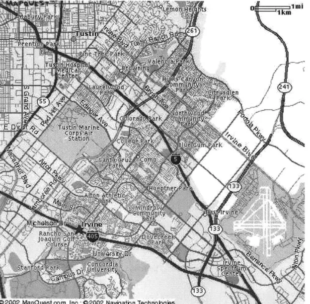
5 Case Studies 59 5.1 The Irvine Data . . . . 59
5.1.1 Network Description . . . . 60
5.1.2 Data Description . . . . 60
5.2 The First Stage of Calibration . . . . 63
5.3 The Second Stage of Calibration . . . . 68
5.4 Network-Level Calibration . . . . 71
5.4.1 The Box Complex Algorithm . . . . 73
5.4.2 The SPSA Algorithm . . . . 75
5.5 R esults . . . . 79
CONTENTS 9
5.7 Summary ... ... 96
6 Conclusion 97
6.1 Research Contribution and Findings ... . 97 6.2 Future Research . . . . 98
A MATLAB Code for the
Box Complex Algorithm 99
List of Figures
1-1 Dynamic Traffic Management Overview . . . . 2-1 Calibrated speed-flow relationship for Interstate 4 in Orlando, Florida
3-1
3-2 3-3
3-4
A Generic Calibration Framework for Traffic Models [15]
Three-stage Calibration Methodology . . . . Sub-network Calibration . . . . Stochasticity in the Supply Simulator Output . . . .
4-1 The White-Box Approach to Simulation Optimization. 4-2 The Black-Box Approach to Simulation Optimization .
5-1 5-2 5-3 5-4 5-5 5-6 5-7 5-8 5-9 5-10
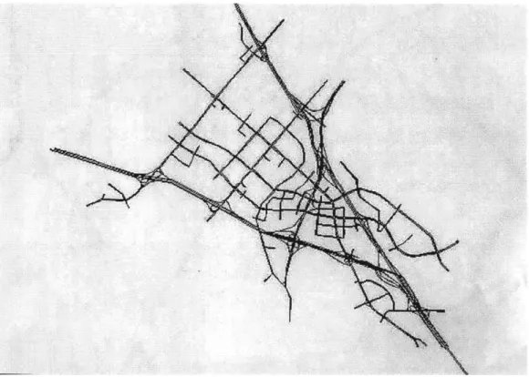
Map of the Study Network Area . . . . The Irvine Network . . . . Primary OD Pairs in the Irvine Network . . 5-day Variability in Arterial Sensor Counts . 5-day Variability in Freeway Sensor Counts . Typical Calibrated Speed-Density Curve . . The SSC Network . . . . Freeway sensor counts on the SSC network Off-ramp sensor counts on the SSC network On-ramp sensor counts on the SSC network
5-11 (Second) off-ramp sensor counts on the SSC network
11 17 26 32 38 40 42 48 49 . . . . 61 . . . . 62 . . . . 64 . . . . 65 . . . . 65 . . . . 67 . . . . 68 . . . . 69 . . . . 69 . . . . 70 . . . . 70
LIST OF FIGURES 5-12 5-13 5-14 5-15 5-16 5-17 5-18 5-19 5-20 5-21 5-22 5-23 5-24 5-25 Averaging Calibrated SSC Network Speeds Comparison
Improving SPSA Performance with Gradient Flows for 04:00-04:15 and 04:15-04:30 . . . .
Flows for 04:30-04:45 and 04:45-05:00 . . . .
Flows for 05:00-05:15 and 05:15-05:30 . . . .
Flows for 05:30-05:45 and 05:45-06:00 . . . .
Flows for 06:00-06:15 and 06:15-06:30 . . . .
Flows for 06:30-06:45 and 06:45:-07:00 . . .
Flows for 07:00-07:15 and 07:15-07:30 . . . . Flows for 07:30-07:45 and 07:45-08:00 . . . .
Flows for 08:00-08:15 and 08:15-08:30 . .
Flows for 08:30-08:45 and 08:45-09:00 . . . .
Convergence of the Box Complex Algorithm Convergence of the SPSA Algorithm . . . .
. . . . 72 . . . . 78 . . . . 82 . . . . 83 . . . . 84 . . . . 85 . . . . 86 . . . . 87 . . . . 88 . . . . 89 . . . . 90 . . . . 91 . . . . 94 . . . . 95 12
List of Tables
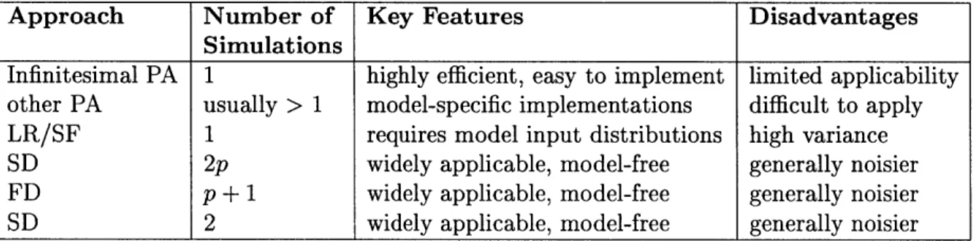
4.1 Gradient Estimation Approaches for Stochastic Approximation (Fu
[11]) . . . . 5 1
5.1 Results of Individual Segment Calibration . . . . 66
5.2 Results of SSC Network Calibration . . . . 71
5.3 Root Mean Square Error values for the Different Optimizations . . . 79
5.4 Calibrated Values Versus Starting Values . . . . 81
5.5 Convergence of the Box Complex Algorithm . . . . 93
5.6 Runtimes of the Box Complex Algorithm . . . . 93
5.7 Runtimes of the SPSA Algorithm . . . . 95
Chapter 1
Introduction
Recent years have witnessed a spurt in the development and deployment of Intelligent Transportation Systems (ITS). Much of the impetus for the development of these systems was derived from a paucity of investment funds, and more importantly, from a lack of public willingness to expand roadway capacity at the cost of detriments to the environment. ITS helps in bolstering the efficiency, productivity and safety of extant transportation infrastructure through the use of the latest data processing, communication and surveillance technologies.
Traffic information devices such as Variable Message Signs (VMS) are now ubiq-uitous; most ITS service providers also provide in-vehicle trip advisory to their sub-scribers regarding accidents and bottlenecks. However, many ITS sub-systems such as Advanced Traffic Management Systems (ATMS), Advanced Traveler Information Systems (ATIS), Advanced Public Transportation Systems (APTS), Commercial Ve-hicle Operations (CVO) and Emergency Management Systems (EMS) would get a much-needed fillip with the ability to assimilate wide-area estimates of prevalent and emerging traffic. Dynamic Traffic Assignment (DTA) systems1 are being developed
to serve this very need for a Traffic Estimation and Prediction System (TrEPS).
'Sometimes synonymously referred to as Dynamic Traffic Management Systems (DTMS) 15
CHAPTER 1. INTRODUCTION
1.1
Dynamic Traffic Assignment (DTA)
The dynamic traffic assignment problem has been the focus of research for more than three decades now ([39], [24], [25], [7]). The advancement of intelligent transportation systems in the last decade has intensified DTA research and led to the development of DTA systems aimed at dynamic traffic management [9], [10], [21], [27].
DTA systems aim to improve general traffic conditions on a proactive basis. Such
systems are designed to address and alleviate traffic congestion using advanced com-munication and surveillance technologies managed by real-time, intelligent software systems. Strategies to ameliorate the congestion call for the use of ITS sub-systems such as ATMS and ATIS.
ATMS refers to control systems that impose constraints on traffic flows. Such
constraints include traffic signal lights (based on fixed timing or on proactive rules), ramp metering, speed limit signs (fixed or variable) and lane use signs. Statutory re-strictions demand drivers' compliance with such systems. ATMS can thereby modify the capacity of the network and affect transportation supply.
ATIS refers to information systems that provide traffic information and travel
rec-ommendations to drivers both before and during their trips. Such guidance may be through means such as radio forecast, web-based or on-board navigation systems and variable message signs. The information provided by these systems may have a bear-ing on drivers' trip-related choices: the decision to travel or not, which destination(s) to travel to, the departure time, the travel mode, and route choice. By influencing drivers' travel decisions, ATIS influence transportation demand.
ATIS differ from ATMS in that drivers are not obligated to follow its prescriptive
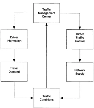
recommendations. Also, an ATMS, designed to control the traffic, is driven by system optimal objectives while an ATIS, designed to influence demand, is driven by user optimal objectives. Figure 1-1 illustrates the roles of ATMS and ATIS in the overall management of a road network and its traffic.
Researchers at MIT have developed the DynaMIT and DynaMIT-P DTA systems.
1.2. DYNAMIT AND DYNAMIT-P Traffic Management Center Direct Driver Traffic Information Control TraveldNtwr
ha bendsine t eid inatafiuangmntcner(M)lnyoupr
CorAoitons
Figure 1-1: Dynamic Tr affic Management Overview
1.2
DynaMIT and DynaMIT-P
DynaMT 2 is a state-of-the-art DTA system designed for real-time traffic estimation
and prediction, and generation of traveler information and route guidance. DynaMIT has been designed to reside in a traffic management center (TMC) and to support
ATIS and ATMS operations.
DynaMIT-P is a DTA-based planning tool developed on the DynaMIT platform. It has been designed to assist transportation planners and policymnakers in assessing possible operational or infrastructural modifications in the local or regional trans-portation networks.
Both DynaMIT and DynaMIT-P use two main simulation tools - the demand simulator and the supply simulator.
The demand simulator is a microscopic simulator that deals mainly with
esti-2
Dynamic Network Assignment for the Management of Information to Travelers
CHAPTER 1. INTRODUCTION
mation and prediction of time-dependent OD flows, demand disaggregation to model the socioeconomic characteristics of drivers, and their decisions of departure time and route choice using (MNL-type) behavioral models.
The supply simulator is a mesoscopic traffic simulator used to simulate vehicular movements 3 on the given network. It can be used to infer traffic flows, queue lengths, speeds, travel times, and densities at all points on the network, and thereby serve to indicate network performance.
1.3
Thesis Focus
The focus of this thesis is the calibration of the supply simulation module within DynaMIT-P.
Calibration is the estimation process to determine correct values of the model parameters, based on traffic measurements. It is aimed at optimally adapting model parameters and coefficients so that the calibrated model is able to replicate field observations to a sufficient level of accuracy.
The calibration process is almost always mated to the process of validation. Val-idation is attempted subsequent to calibration: the objective is to test whether the calibrated model is able to reproduce field observations to a sufficient level of accuracy, both from a qualitative and quantitative point of view.
The importance of the calibration and validation of models in efficient and correct model application studies cannot be overstated. Regular updating model parameters and relations affords ever-increasing accuracy in modeling results. A congestion-related study by the Dutch Ministry of Transport
[33]
concludes that models are seldom exhaustively calibrated and validated (if at all!) for their considered applica-tion.3
also referred to as 1. network performance, or 2. traffic dynamics, or 3. flow propagation elsewhere in this document
1.4. THESIS OUTLINE
1.4
Thesis Outline
The remainder of this thesis is organized as follows: Chapter 2 explores the literature related to calibration of traffic simulation models. More specifically, it dwells on the calibration of the components of a DTA system, especially the traffic dynamics sim-ulation models.
Chapter 3 outlines a methodology for the calibration of mesoscopic flow propagation models on the basis of the literature reviewed.
Chapter 4 discusses the topic of simulation optimization in light of the optimization-pronged attack needed to tackle the calibration problem. Different stochastic opti-mization algorithms are looked into, and this exercise is used to identify the algorithms that will be used for the calibration purpose on hand.
Chapter 5 presents case studies. It begins by outlining a three-stage calibration methodology, and then employs a random search algorithm (the Box Complex al-gorithm) and a path search algorithm (the Simultaneous Perturbation Stochastic Approximation algorithm) for calibration of a large real network.
A summary of the research and directions for further work are presented in the final
chapter.
Chapter 2
Literature Review
The objective of this chapter is to study the different approaches employed by re-searchers in calibrating traffic simulation models. This literature review is used to avoid the pitfalls, overcome the deficiencies and adopt the plus-points of past ap-proaches in the calibration methodology we will outline and implement.
2.1
Development of Traffic Models
Traffic model development usually follows the lines of:
1. Establishing and testing theories on the basis of microscopic/macroscopic traffic
flow observations, either by inductive or by deductive means. This involves developing qualitative and mathematical relations based on empirical knowledge and qualitative data analysis.1
2. Calibration of the models for a specific application using empirical data.
'also referred to as
A. Model verification - process of determining how well the underlying model theory and logic reflect reality, and
B. Model validation - process of determining if the proposed model logic is correctly represented by the computer code
CHAPTER 2. LITERATURE REVIEW
3. Validation of the calibrated models using different data
2.2
Data sources
This section briefly touches upon the different infrastructure-based and non-infrastructure-based data sources.
2.2.1
Infrastructure-based detectors
The infrastructure-based detector systems are of two types: the inductive loop-based systems and the video, infrared and radar systems. Loop-based systems can provide either lane-aggregate or lane-specific speeds and flow-rates at varying frequencies (minute-aggregate/hour-average etc. depending on the type of loop-based system). Some such systems also enable collection of individual vehicle data. Video, radar and infrared techniques are used to collect individual vehicle data (from which macroscopic data can be determined) in a small region. However, these are not as accurate as the loop-based systems.
2.2.2
Non-infrastructure-based detectors
This category refers to the use of vehicles themselves being used for data collection purposes. Such probe vehicles are equipped with board computers (OBC) or on-board units (OBU) from which positioning (via GPS) and speed measurements may be obtained. Combining probe trajectories with fixed detector data allows for the estimation of flow characteristics of non-equipped vehicles.
Alternatively, aerial photographs and video data can be collected. With suffi-ciently detailed data, densities can be directly determined. Also, quantities such as space-mean-speeds and distance-headways can be determined by comparing pho-tographs of consecutive time instants.
2.3. TRAFFIC MODEL PARAMETERS
2.3
Traffic Model Parameters
Traffic simulation models are usually classified as macroscopic, mesoscopic or micro-scopic on the basis of the level of detail of simulation.
Macroscopic and mesoscopic models use the analogy between vehicular flow and fluid flow. When compared to microscopic models, the number of unknown model
relations and parameter relations is relatively low.
Calibration of first-order macroscopic and mesoscopic models requires the
con-struction of speed-density (or flow-density) curves - mesoscopic models do, of course, require a more detailed modeling relationship (with more governing parameters) than
macroscopic models. Traffic data covering the congestion spectrum from free-flow to congested flow ensures a complete fundamental diagram.
Higher-order and microscopically-based models require estimation techniques for model parameters other than those implicit in speed-density curves. For instance, the constant anticipation factor co reflects the spread in velocities while a so-called
viscosity coefficient captures the transition rate from brisk to careful driving. To
determine co, one needs to either
1. determine the velocity of shockwave propagation, or
2. use speed variances
In general, macroscopic model calibration is relatively straightforward relative to the microscopic case.
Calibration of microscopic models is concerned with tuning parameters that
deter-mine vehicle-vehicle interactions, such as the ones in car-following and lane-changing
models of driver behavior.
The relatively large number of parameters dictates that complex microscopic
mod-els should be dis-assembled, calibrated and tested in a step-by-step fashion, whenever
possible. Sometimes the number of degrees of freedom in a microscopic model is so
CHAPTER 2. LITERATURE REVIEW
large that multiple parameter value combinations yield the same model behavior. To aid microscopic model calibration, sensitivity analysis can be performed.
Data requirements for microscopic model calibration are very stringent, in that individual vehicle data in the form of trajectories and pair-wise vehicle dependency data are needed. In contrast, data requirement criteria for model validation are less stringent - they need reflect only the specific traffic flow behaviors that the calibrated model is expected to describe.
2.4
Calibration of Traffic Simulation Models
While there is no dearth of literature on the calibration of stand-alone microscopic traffic simulation models, literature on calibration of traffic simulation models in a
DTA setting is sorely lacking. We review some of the literature as regards
calibra-tion of traffic simulacalibra-tion models, especially the calibracalibra-tion of mesoscopic/macroscopic traffic dynamics simulation models in DTA systems.
Hellinga [15] provides an excellent discussion of the requirements for the calibra-tion of traffic simulacalibra-tion models. The paper tries to address the key issue of what constitutes adequate model calibration and what measures of performance (MOPs) should be used in calibration. The author argues that a model can be deemed to be calibrated if its outputs are comparable to field data and meet pre-specified cal-ibration criteria established prior to the commencement of any modeling. Some of the potential MOPs listed are: link volume, link speed, link travel time, queue size and location, trip travel time by origin, destination, and departure time, total travel time, average trip length, average fuel consumption, tailpipe emissions and average accident risk. The author also points out that sufficient field data to quantify statis-tical confidence limits on the MOP(s) of interest are very rarely available, and this lack thereof rules out such a rigorous statistical approach. Consequently, it is not uncommon to see the use of terms such as reasonable, adequate, and representative 24
2.4. CALIBRATION OF TRAFFIC SIMULATION MODELS
when referring to the adequacy of calibration.
The author addresses the loss of accuracy in network modeling when choices have to be made on the spatial extents of the network and on source/sink zones. The paper briefly dwells upon the correct specification of macroscopic speed-density relationships and points out how it is beneficial to classify links into several categories and specify a unique speed-density relationship for each category rather than for each individual link. This idea is carried forth in the current research where similar road segments are grouped together for the purpose of calibration. Also pointed out is the fact that free speed is likely the least critical parameter, since it can be estimated with reasonable accuracy from the mandated speed limit itself. It is stressed that the impacts of speed at capacity flow, the capacity and the jam density are far more significant as they influence the formation, extent and dissipation of queues.
Route choice behavior is yet another aspect of calibration for networks where the drivers have more than one viable route choice. Field data to capture route choice can rarely be obtained; an inappropriate route choice parameter value can annul the accurate calibration of all other parameters. And finally, O-D demands, a must as input for nearly all simulation models, cannot be directly observed and must be derived via other means, most commonly from link flows.
The paper concludes by pointing out that simulation results are often incorrect because of the use of an insufficiently validated and verified model on the part of the model developer or an incorrectly calibrated model on the part of the user. It recommends a clearly and realistically defined data collection process for minimal negative impact on the model user's calibration process.
Kurian [19] uses an experimental design methodology to identify the set of sensitive parameters in the car-following model in MITSIM, a microscopic traffic simulator. He uses an optimization-based framework and two forms of an objective function to quantify the deviation between observed and simulated values. Stochasticity is shown to have a very significant impact on the optimal parameter values. The thesis
26 CHAPTER 2. LITERATURE REVIEW 100 Freespeed 87.2 km/h 40 Speud.W-apagity 70.8 kruh * Capachy =1925,0 VPh 30' Jamdensity =621va/l/km 20-10 500 100 1500 200 Flow (vphlVane)
Figure 2-1: Calibrated speed-flow relationship for Interstate 4 in Orlando, Florida (Van Aerde and Rakha [1])
concludes with a very strong endorsement of calibration studies, mentioning that
simulation performance was significantly enhanced by appropriate calibration. Darda [8] has developed a module for joint model parameter calibration and OD estimation in the MITSIM microscopic traffic simulator. Again, an optimization-based framework driven through the Box Complex algorithm is used while taking into account the interaction between various model parameters and OD flows.
Van Aerde and Rakha [1] have carried out calibration of speed-flow relationships
using loop detector data aggregated to a 5-minute average. Figure 2-1 shows the parameter values corresponding to the curve fitted for Interstate 4 in Orlando, Florida.
Such curve-fitting exercises, however, cannot be carried out for realistically sized networks with hundreds of segments; the issue is not the prohibitively large number
of segments, more a lack of data!
Jayakrishnan et al [16] discuss calibration issues concerning microscopic simulation
2.4. CALIBRATION OF TRAFFIC SIMULATION MODELS
a microscopic traffic simulator, is integrated with the routing and behavior response schemes in the DYNASMART mesoscopic model. The calibration scheme uses a weighted least squares objective function to match simulated values with field data. However the termination criterion is described as
If the comparisons between observed and modeled value comparisons (sic)
are within recommended guidelines and the graphic visualisation of vehi-cles is realistic, then the model is deemed calibrated.
Wall et al [38] perform calibration of a microscopic model with the intent of using it in conjunction with real-time loop detector data to predict downstream traffic volumes and speeds. The calibration is performed in a least squares sense of matching model output with observed data. The model parameters are updated using a finite difference approximation for the differential.
Mahmassani and Tavana [22] use transfer function methods to capture the dy-namic characteristics of speed-density time series data, including the existence of serial correlation, in the specification and estimation of dynamic speed-density rela-tions for traffic simulation and ATMS applicarela-tions.
The prevailing speed at any location is surmised to be a function of past values of speed, density and traffic conditions upstream and downstream. The general model is represented as
ut,X = (y, ), k (, Ue[k(q)
where
Ut,,= speed at time t and location x,
u(r, ) = distribution of speed values over space, , and time 7
k(71,) = distribution of density over space, , and time q
ue[k(q)] = static equilibrium speed for a given density,
which in turn itself can be a function of the flow, q.
CHAPTER 2. LITERATURE REVIEW
In the context of data received at an ATMS control center, the above relationship is operationalized as
= f [uth, kt-, Ue(k-h), a-h] j, h c {0, 1, 2, 3, ...}
where
Zai= shock introduced to the system at time t and location i. The authors show that transfer function methods outperform 2 regression calibration
models when the equilibrium speed-density relationship is assumed to be known (the dependent variable is taken to be the absolute value of the differenced speed varia-tion). They also claim tranferability of the model to new sites I without the need for recalibration. Furthermore, it is conjectured that even though traffic conditions at the selected site were in the uncongested regime, transfer function models will exhibit even better performance under congested conditions in which dynamic effects are more significant.
It is worth emphasizing that calibration of transfer function models would need very detailed data. Also, if we are to include spatial effects, we need a closely spaced set of sensors. Finally, the above research was based upon data from freeway sen-sors and applicability of transfer function models to wide-area networks needs further investigation. Nevertheless, transfer function models hold much promise in online calibration for the purpose of supporting real-time operational decisions. They could be one of the strategies for mining expansive real-time traffic databases.
He et al [14] outline a three-step framework for the calibration of an analytical DTA model. Assuming knowledge of OD trip tables, they propose sequential calibration
of:
1. Dynamic Link Travel Time Functions
2
In their analysis of data obtained at a single station on Interstate 10, the authors ignore spatial effects (j = 0).
3The other site was also in the San Antonio region.
2.4. CALIBRATION OF TRAFFIC SIMULATION MODELS
2. Route Choice Model
3. Flow Propagation
with 1 and 2 being implemented offline or online and 3 being implemented online. For offline calibration, the authors assume availability of adequate surveillance data and survey data of route choice, traveler demographics, travel times and flow propa-gation. They propose calibration of linear or nonlinear link travel time formulae for different types of links: freeway links, pre-timed signalized links, actuated signalized links, stop-controlled links etc. They also postulate that various route choice formulae could be calibrated offline for different types of travelers.
For the online calibration of dynamic link travel time functions, the authors propose introduction of an error term for fitting their proposed formulae with detector data. They propose use of the maximum likelihood method for online calibration of route choice, again contingent of the availability of "sufficient route choice data". The on-line calibration of flow propagation is also proposed to be carried out by adjustment via an error term.
A major weakness of the proposed methodology is that it is heavily reliant on a rich
archive/supply of data and the calibration suggestions are heavily qualified with "can be". The test network used to illustrate the methodology is a very simplistic 3 X 3 Manhattan metric of freewat links and assumes prior knowledge of time-dependent
OD matrices, a very restrictive assumption for the purpose of DTA. The scalability
of this methodology to heterogeneous realistically-sized networks is not investigated. Hawas [13] ranks individual DTA components to determine the order in which cal-ibration should be performed. However, he ignores the interaction between individual components that is the prime essence of any DTA system. A further weakness of this research is that the case study uses the components of a traffic simulator rather than
a DTA system.
Balakrishna [3] addresses the overall problem of jointly calibrating the OD esti-mation and route choice models in the demand simulation component of the DTA
30 CHAPTER 2. LITERATURE REVIEW
prototype DynaMIT.
2.5
Conclusion
The literature reviewed indicates the need for a systematic calibration of the traffic dynamics simulator in a DTA system. Drawing upon the ideas of past research investigations, the next chapter outlines a calibration methodology customized for the calibration of the supply simulation module in DynaMIT.
Chapter 3
Calibration Methodology
This chapter starts with a blueprint for an "ideal" calibration methodology and then proposes one for our own problem so that it adheres to the same. In so doing, we draw heavily on the approaches used by researchers cited in the last chapter while factoring in the characteristics unique to our mesoscopic traffic dynamics simulator, the network of interest, and the dataset.
3.1
Ideal Calibration Methodology
Guidelines for the calibration and validation of traffic simulation models are out-lined in [30] and [26]. An unambiguous, clear, structured and operational calibration methodology would ideally include the following, interdependent stages:
1. Identification of model application area
2. Determination of assessment objectives
3. Determination of performance measures: definition of performance indicator,
its calculation, nature of the indicator in terms of the effect it aims to quantify, scope of the indicator and data collection needs
32 CHAPTER 3. CALIBRATION METHODOLOGY
Study Definition
Define Study Purpose & Goals
10 Criteria lo Measures of Performance Field Data L -.-.- -.-.--- --- --- ---.--- ---- - -- --- - ---Initial Calibration -Network
-speed-flow -o SIMULATION MODEL -demand
-driver/vehicle
Output --- Evaluation Compare to criteria
Criteria met
Criteria not met
- Re-calibrate 4 Evaluation
Initial Calibration Evaluation of Model Outputs
3.2. CALIBRATION OF THE DYNAMIT SYSTEM
4. Description of general tools for calibration, e.g. sensitivity analysis, step-by-step
calibration, mathematical programming algorithms, t-tests, analysis of variance
5. Overall definition of success 6. Experimental set-up
The main advantage of such a methodology is the systematically organized
cali-bration and validation process, and a vantage ground for cross-comparison between
models. Figure 3-1 shows a generic three-phase, eight-component calibration
frame-work for traffic models (Hellinga [15]).
The first phase comprises exercises such as definition of study goals, identification
of data requirements vis-a-vis the field data available, identification of measures of
performance consistent with the objectives of the study, and of simulation capabilities;
and the specification of criteria to evaluate the calibration. All these activities are
undertaken prior to the commencement of any modeling.
The second phase involves the actual calibration - namely the representation of the network, the macroscopic speed-density (or speed-flow) relationships, driver behavior
models and estimation of O-D flows.
In the last phase, the results from the model are compared with field data and
against the pre-specified criteria. If the model meets these criteria, it is deemed to be
adequately calibrated and is ready for testing non-base-case scenarios. If, however, the model is found to be wanting in meeting these pre-specified criteria, refinements
and/or modifications, and sometimes even a recalibration from scratch must be done.
3.2
Calibration of the DynaMIT system
In the current context, we are interested in calibrating the DynaMIT system. A
holistic calibration of the DynaMIT system involves joint calibration of the demand
and supply simulators. The current research assumes the availability of a calibrated
CHAPTER 3. CALIBRATION METHODOLOGY
demand simulator and focuses exclusively on the calibration of the supply simulator, which we describe next. For the sake of completeness, however, we also enumerate the demand simulation parameters at the end of this section.
3.2.1 Supply Simulator Parameters
The supply simulator in DynaMIT is a mesoscopic traffic simulator that simulates vehicular movements and provides metrics of network performance such as the tem-poral evolution of flows, speeds, densities, queue lengths, and travel times at all points on the network.
The supply simulator obtains the network description and the list of packets to be moved on the network through its interfaces with the network topology component and the list of packets component respectively. It then simulates the movement of vehicles on the network for the given supply simulation time interval.
The network consists of a set of nodes, links and loading elements (loaders). The nodes correspond to the intersections or merge points in the actual network, while links represent the unidirectional pathways between them. Loading elements repre-sent areas where traffic is generated and/or attracted. The links in the network are subdivided into segments to capture changing geometries. Further, the lanes within each segment are grouped into lane groups to account for turn-specific capacities at
diversions/merge points and intersections.
Unlike microscopic simulators, there are no lane-changing or car-following models; lanes are used primarily to capture queuing behavior. There is also the concept of packets, whereby two or more vehicles having the same origin and destination are aggregated - the simulator concentrates on aggregate results rather than modeling individual vehicle behavior. Detailed mesoscopic models are used to capture traffic dynamics and accurately model the formation and dissipation of queues, i.e. there are two major models: 1. a deterministic queuing model and, 2. a speed model.
The queuing model, with the ability to explicitly model spillbacks, makes heavy 34
3.2. CALIBRATION OF THE DYNAMIT SYSTEM
use of the input and output capacities of individual segments; the movement of vehi-cles from one segment to the next is governed by a host of capacity calculations and the physical space available on the downstream segment. Furthermore, capacities are also used to accurately model incidents and signalized controls at intersections.
Flow propagation is based on the following aggregate speed-density relationship
u =max (Umin, Ucai)
u1 , if k < ko
Ucal
u1[1 - ( kjam)], otherwise where
u = speed (mph),
Umin = minimum speed,
Ucal = speed calculated as per the two-regime equation,
Uf = free-flow speed,
k = density,
ko= maximum density at which free-flow is possible, kjam = jam density,
a= parameter,
#3
= parameter.The simulation of the traffic network operations proceeds in a number of update phases. Nested within each update phase are a number of advance phases. The update phase is used to update the dynamic traffic characteristics (e.g. speeds, den-sities, capacities) whereas the advance phase is used to advance vehicles to their new positions.
Depending on the demands of the application, the supply simulator can be oper-ated at different levels of granularity - this flexibility allows for a full investigation
CHAPTER 3. CALIBRATION METHODOLOGY
of tradeoffs between accuracy and run-time efficiency, and facilitates the selection of the most suitable combination for each case.
We list below the parameters that are key to calibrating the supply simulator:
" Segment-specific speed-density parameters Uf, Umin, ko, kjam, a, and , * Lane group capacities on freeway and arterial segments, and
* Lane group capacities at the signalized intersections.
3.2.2
Demand Simulator Parameters
The demand simulation parameters are those embedded in the O-D estimation (and prediction) module, and the route choice model parameters.
Route Choice Parameters
The key calibration parameters for the route choice model are:
" Parameters in the path choice set generation algorithm
* Parameters in the path utility specification
" Path-size exponent -y
O-D Estimation (and Prediction) Parameters
The key calibration parameters in the O-D estimation (and prediction) module are:
* The historical database of O-D flows, xH
h
The variance-covariance matrix Vh associated with indirect measurement errors
* The variance-covariance matrix Wh associated with direct measurement errors
* The matrices fh of autoregressive factors.
For further details, the reader is referred to Balakrishna [3] and Ashok [2].
3.3. PROPOSED CALIBRATION METHODOLOGY
3.3
Proposed Calibration Methodology
Being comprised of a demand microsimulation model and a mesoscopic supply simu-lation model, a holistic calibration of the DynaMIT system would need to proceed in a two-stage iterative loop. We reiterate that the calibration methodology we propose will focus solely on the calibration of the supply simulator; it is assumed that the demand simulator has been adequately calibrated separately.
In proposing a calibration methodology of our own, we would like to use the following ideas encountered in the literature review:
" Calibration of speed-density relationships for individual segments using the
curve-fitting approach for loop detector data, as done in Van Aerde and Rakha [1].
" Classification of sgements into categories, with a unique speed-density
relation-ship for each category rather than for each individual segment (Hellinga [15]).
" Performing calibration in the least squares sense of matching model output with
observed data (Wall et al [38]), or better still, using a weighted least squares objective function to match simulated values with field data, as outlined in Jayakrishnan et al [16].
These ideas motivate us to carry out the calibration exercise in three different, se-quential stages at three correspondingly different levels of aggregation.
3.3.1
Three-stage Calibration
As shown in Figure 3-2, the calibration of the supply simulator for a large-sized real network is done at the following levels:
disaggregate level This involves calibration of the speed-density relationships and capacities at the level of each individual segment. The capacities of the
CHAPTER 3. CALIBRATION METHODOLOGY
Traffic sensor data
Subnetwork
calibration
True O-D flows,
Route Choice
Initial parameter values
System level calibration
Supply
Demand
Figure 3-2: Three-stage Calibration Methodology
Calibration of individual elements
1. Speed-density relationships
of segments
2. Capacities of segments
(accounting for intersections)
3.3. PROPOSED CALIBRATION METHODOLOGY
sections are also individually calibrated. Such a calibration assumes that there is no interaction between contiguous segments.
sub-network level This involves calibration of a sub-network where origin-destination flows can be accurately estimated from the sensor counts and there are very lim-ited or no route choice possibilities. However, the subnetwork should consist of links and intersections with several interactions. Using such a sub-network enables us to carry out the simulation without the errors inherent in demand estimation in the presence of route choice.
The schematic in Figure 3-3 outlines such a sub-network calibration.
entire network level Finally, the calibration is done at the level of the entire net-work. This takes into account all the interactions that come into play between the various segments. Such a calibration takes care of the stochasticities and errors arising out of the demand estimation.
3.3.2 The Tool for Calibration
Before deciding upon the technique that needs to be used to tackle the calibration of the supply simulator, we need to emphasize the two most vital characteristics of this problem:
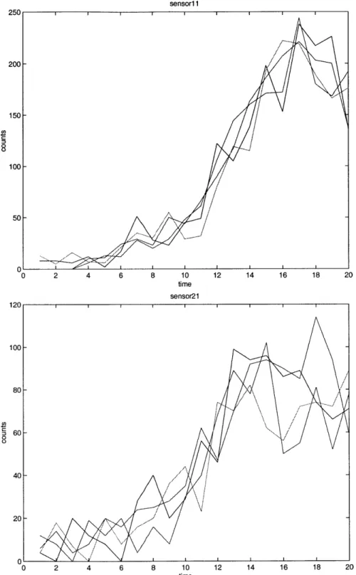
Noisy Output Like most simulation models, the supply simulator in DynaMIT too is a stochastic model' that uses random numbers to generate a sequence of stochastic values. It is therefore very important to realize that each simulation result is only a single point in a wide distribution of values. In fact, stud-ies of NETSIM have indicated that misleading results will be obtained if the variability of the simulation results is ignored (Benekohal et al [5]).
'Strictly speaking, the variation in the simulated flows is due to the stochasticity in the departure times and less of an attribute of the supply simulator models
CHAPTER 3. CALIBRATION METHODOLOGY
(
Traffic sensor data
Initial parameters
run DynaMIT on
sub-network
+Updateparameters
4
Initial parameter values
NO
convergence of flows
and speeds?
YES
STOP
Figure 3-3: Sub-network Calibration
Calibrated O-D
flows and
Route Choice
3.3. PROPOSED CALIBRATION METHODOLOGY
Figure 3-4 underlines this important facet of the supply simulator - the graphs represent simulated flows of two sensors in the Irvine study network, as recorded over four simulations.
Problem Dimension A traffic simulation network usually has a very large number (typically in the hundreds) of segments. Calibration of the entire study network requires the calibration of the 7-tuple
{uf, kj,, a, #, capacity, Umin, ko}
for each and every segment in the network - a very large hyperspace.
The supply simulator calibration problem thereby lends itself to mathematical programming techniques; more specifically, we need to use a stochastic optimization technique. In the following chapter, we examine some of the stochastic optimization techniques that can be used for simulation optimization.
CHAPTER 3. CALIBRATION METHODOLOGY 25 20 15 sensori 1 0 f 0-0 /7 / 0 2 4 6 8 10 12 14 16 18 20 time sensor21 I on 10 5 0 0 100- 80- 60- 40- 20-0 0 2 4 6 8 10 12 14 16 18 20 time
Figure 3-4: Stochasticity in the Supply Simulator Output
42 8i -\ \ \ / / \/
Chapter 4
Stochastic Optimization
The most commonly used optimization techniques - linear, nonlinear and (mixed) integer programming - require an explicit objective function. The stochastic context of simulation, however, defies analytical tractability, and thereby precludes the direct use of the expanse of optimization methods suited for solving deterministic problems. The reader is referred to Law and Kelton [20] and Andradottir [4] for recent literature on simulation optimization. Fu [12] provides an excellent exposition of simulation optimization. This chapter discusses the various methods of stochastic optimization.
4.1
Stochastic Optimization of Simulation Systems
Stochastic optimization refers to optimization of systems that produce output with inherent system noise. A simulation optimization problem is one where the objec-tive function and some constraint(s) are implicit, stochastic functions of the decision parameters of the system, and as such, can be evaluated only by computer simulation.
4.1.1 Issues
Absence of analytical expressions of the objective functions and/or constraints elim-inates the possibility of differentiation and exact calculation of local gradients. Also,
CHAPTER 4. STOCHASTIC OPTIMIZATION
stochasticity means that we cannot decide upon the best point in the sample space by evaluating the objective function at the points of interest merely once. Furthermore, running computer-simulation programs is far more time-intensive than evaluating an-alytical functions and there is a great premium on the efficiency of the optimization algorithms. Lastly, interfacing generic optimization toolboxes with the simulation package is no mean feat, especially so since the simulation modeling language is, more often than not, different from the optimization programming language.
4.1.2 Notation
To discuss the various methods of stochastic optimization, the notation we use as-sumes that the optimization problem is of the form
min 1(0),
where
0 = the controllable set of parameters,
6 = the constraint set on 0,
1(0) = the objective function.
The objective function is an expectation , i.e.,
1(0) = E[L(0,w)],
where
W = a sample path (or simulation replication),
L(0, w) = corresponding sample performance estimate.
4.2. PATH SEARCH METHODS 4.1.3 Classification
The different approaches of searching for an optimum may be classified into three major categories: path search methods, pattern search methods, and random meth-ods. Path search methods have been the most widely studied approach for solving the simulation optimization problem, and the section devoted to the same is more detailed than the others.
4.2
Path search methods
Path search methods involve the estimation of a direction to move from the current vector of parameters to an improved point in the feasible region. The most common direction of movement is the gradient.
4.2.1 Response Surface Methodology
Response Surface Methodology (RSM) is a widely studied approach that tries to locally fit a polynomial response surface model to a set of sample observations in a particular region of the search space. The choice of these observation points is made
by experimental design techniques, and the polynomial that is fitted is usually of first
or second order. RSM is applied to the problem of simulation optimization either in the form of 1. metamodels, or 2. sequential procedures.
Sequential RSM involves fitting a linear regression model around a given parameter setting, defining a linear response surface from the ordinary least squares estimate, and moving in the direction of the gradient until the linear response surface stops improving the response function value. Phase II is then implemented by fitting a quadratic model to the response, and the same procedure as Phase I, namely moving in the gradient direction, is performed until the magnitude of the gradient becomes sufficiently close to zero. If need be, higher degree regression models can then be utilized in analogous manner. Smith has developed an automatic optimum-seeking 45
CHAPTER 4. STOCHASTIC OPTIMIZATION
program based on RSM that can be interfaced with independently built simulation models. The reader is referred to Safizadeh [32] for more details.
Using a metamodel simply means two separate problems of estimation and opti-mization. After choosing points 0 based on a statistical design of experiments method-ology, the outputs at these points are used to fit a response curve or metamodel. This functional relationship between the output and the simulation paramters is then opti-mized using deterministic procedures. An extensive discussion of metamodels is given in Kleijnen [18].
RSM has the advantages of being based on sound statistical theory that is easily understood, and of ease of implementation. The disadvantage is that a large number of simulation runs are needed. Also, it has been shown to be inadequate for complex functions with sharp ridges and flat valleys.
4.2.2 Stochastic Approximation
Stochastic Approximation (SA) is another path search method. The basic underlying principle is that the optimization problem can be solved by finding the zero of the gradient. The general form of the stochastic algorithm is given by
On1 = Hr(On - anVL(0n)) where
On= parameter value at the beginning of iteration n, VL(0n) = estimate of VL(0n) from iteration n ,
{an}
= positive sequence of step-size multipliers (gain sequence),ie = projection onto 8, the constraint set on 0.
When an unbiased estimator is used for VL(0n), the algorithm is called a Robbins-Monro algorithm [31] and when a finite difference estimate is used, the algorithm is called a Kiefer-Wolfowitz algortithm [17]. The optimal asymptotic convergence rates 46
4.2. PATH SEARCH METHODS
are p-1/2 for the Robbins-Monro algorithm, and p1/3 (p-1/4) for the Kiefer-Wolfowitz
symmetric (one-sided) differences1 (Pflug [29]).
Convergence The pivotal question to investigate is whether the iterate On
con-verges to 0* as n gets large. The rich convergence theory developed for SA over the years makes it possible to formally establish convergence2 for any stochastic optimiza-tion algorithm of the SA form.
One of the many sufficient conditions given for a.s. convergence involves the definition of an underlying ordinary differential equation that roughly emulates the
SA algorithm for large n and disappearing random effects. It turns out that the
convergence properties of this deterministic differential equation are closely related to the stochastic convergence properties of the general SA equation.
The most famous of the convergence conditions for SA are based upon the gain sequence {an}. The conditions perform a tightrope act of not damping out the noise effects as we near the solution (an -+ 0) and, at the same time, avoiding premature (false) convergence of the algorithm (E' an = 00). The scaled harmonic sequence
{
},
a > 0, is the best-known example of a gain sequence that satisfies the gain conditions (and, is an optimal choice with respect to the theoretical rate of con-vergence, although in practice other decay rates may be superior in finite samples). Usually some numerical analysis needs to be done before deciding upon the best scale factor for the gain sequence decay. Other important convergence criteria relate to the smoothness of the objective function, the magnitude of the noise, and the initial position.Also of importance is the probability distribution of the iterate which happens to be a random vector in a stochastic setting. Having knowledge of the distribution provides key insight into two major aspects: (1) error bounds for the iterate, and (2)
ip is the dimension of the parameter vector.
2Convergence is in the probabilistic sense in the stochastic context. The most common form of convergence established for SA is in the almost sure (a.s.) sense.
CHAPTER 4. STOCHASTIC OPTIMIZATION
SIMULATION PROGRAM AS WHITE BOX
Input Parameter Simulation Output
OPTIMIZATION PART
updated input parameter
estimate of the gradient
4-Figure 4-1: The White-Box Approach to Simulation Optimization
guidance in the choice of the optimal gain sequence {an} so as to minimize the likely
deviation of 0n from 0*.
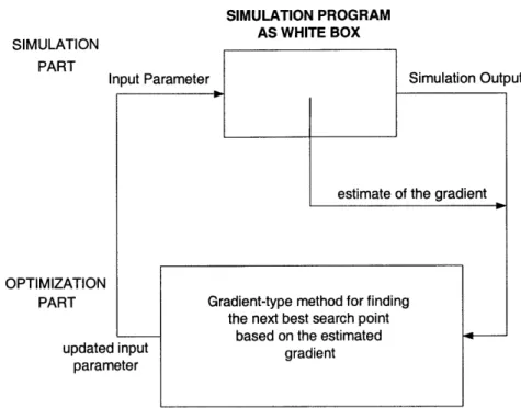
"White Box" Approaches Approaches that provide an unbiased estimator of the
gradient rely on some knowledge of the system being studied, and include techniques such as perturbation analysis, the likelihood ratio/score function method, and weak derivatives. Since these approaches require knowledge of the underlying system, they are referred to as "white box" approaches to simulation optimization. Figure 4-1 shows the white-box approach.
"Black Box" Approaches Figure 4-2 shows the black-box approach. When the
simulator needs to be treated as a black box, the usual approach is to use finite differences, either one-sided (FD) or symmetrical (SD), given respectively by:
[L(0. + cnei, ) - L(n, )]/cn,
48
SIMULATION
PART
Gradient-type method for finding the next best search point
based on the estimated gradient
4.2. PATH SEARCH METHODS SIMULATION PART Input Parameter Experin nex OPTIMIZATION PART 49 SIMULATION PROGRAM AS BLACK BOX Simulation Output
Figure 4-2: The Black-Box Approach to Simulation Optimization
[L(O, + cei, w"+) - L(O, - cej, wi-)]/2c., where
= unit vector in the ith direction,
= positive sequence converging to zero,
= pair of sample paths (simulation replications) used for the ith component of the nth iterate of the algorithm,
= original sample path (replication) used to estimate the performance measure itself.
In both cases, the estimate requires O(p) (p is the dimension of the parameter vector) simulation replications.
Newer approaches that treat the simulator as a black box include harmonic differ-ences based on frequency domain experimentation and simultaneous perturbations.
A frequency domain experiment is one where selected input parameters are oscillated
mental design method for finding the t best search point based on the nformation about the sample
performance estimates gathered so far ej {cn
![Figure 2-1: Calibrated speed-flow relationship for Interstate 4 in Orlando, Florida (Van Aerde and Rakha [1])](https://thumb-eu.123doks.com/thumbv2/123doknet/14195040.478898/26.918.226.746.171.533/figure-calibrated-relationship-interstate-orlando-florida-aerde-rakha.webp)
![Figure 3-1: A Generic Calibration Framework for Traffic Models [15]](https://thumb-eu.123doks.com/thumbv2/123doknet/14195040.478898/32.918.146.802.210.974/figure-a-generic-calibration-framework-traffic-models.webp)

![Figure 4-2: The Black-Box Approach to Simulation Optimization [L(O, + cei, w"+) - L(O, - cej, wi-)]/2c.,](https://thumb-eu.123doks.com/thumbv2/123doknet/14195040.478898/49.918.187.779.157.563/figure-black-box-approach-simulation-optimization-cei-cej.webp)