Predicting failures in complex multi-tier systems

(1)

Predicting Failures in Complex Multi-Tier Systems

Doctoral Dissertation submitted to the

Faculty of Informatics of the Università della Svizzera italiana in partial fulfillment of the requirements for the degree of

Doctor of Philosophy

presented by

Rui Xin

under the supervision of

Prof. Mauro Pezzè

(2)

(3)

Dissertation Committee

Prof. Walter Binder USI Università della Svizzera italiana, Switzerland

Prof. Cesare Pautasso USI Università della Svizzera italiana, Switzerland

Prof. Holger Giese University of Potsdam

Prof. Rogério de Lemos University of Kent

Dissertation accepted on 18 November 2020

Prof. Mauro Pezzè

Research Advisor

USI Università della Svizzera italiana, Switzerland

Prof. Walter Binder Prof. Silvia Santini

PhD Program Director PhD Program Director

(4)

I certify that except where due acknowledgement has been given, the work presented in this thesis is that of the author alone; the work has not been submitted previously, in whole or in part, to qualify for any other academic award; and the content of the thesis is the result of work which has been carried out since the official commencement date of the approved research program.

Rui Xin

Lugano, 18 November 2020

(5)

Abstract

Complex multi-tier systems are composed of many distributed machines, feature multi-layer architecture and offer different types of services. Shared complex multi-tier systems, such as cloud systems, reduce costs and improves resource utilization efficiency, with a considerable amount of complexity and dynamics that challenge the reliability of the system.

The new challenges of complex multi-tier systems motivate a new holistic self-healing ap-proach, which must be accurate, lightweight and proactive, to ensure reliable cloud applications. Self-healing techniques work at runtime, thus they offer automatic and flexible ways to increase reliability by detecting errors, diagnosing errors, and either fixing the errors or mitigating their effects. Self-Healing Systems leverage the time between the activation of a fault and the failure by taking actions to avoid failures. Self-Healing systems shall predict failures, localize the faults and fix or mask them before the failure occurrence.

In my Ph.D, I focused on predicting failures and localizing faults. In this thesis I present an approach, DyFAULT, that predicts failures by detecting anomalous systems states early enough to diagnose the causing errors and fix them before the failure occurrence, and localizes faults by leveraging the collected data to pinpoint the location of error and possibly the type of the fault. The contribution of my Ph.D work includes: (i) an approach to accurately predict failures and localize faults that requires training with fault seeding. (ii) an approach to predict failures and localize faults that requires training with data from normal execution only. (iii) a prototype implementation of the two approaches (iv) a set of experimental results that evaluate the proposed approaches of DyFAULT.

(6)

(7)

Acknowledgements

I would like to express my thanks to my advisor, Prof. Mauro Pezzè, for his thorough support in guiding the project and improving my academic skills. Without his considerate help in both work and life, I would not have been able to complete this research.

I also would like to thank a few researchers from Università della Svizzera italiana, including Prof. Antonio Carzaniga, Prof. Walter Binder, and my colleagues in the STAR research group, for many talks that extended my knowledge and inspired my philosophical thoughts.

Thanks also to Yudi Zheng, Haiyang Sun and Jingjing Lin, who helped me out when I had personal issues in the midst of my thesis writing.

The four and a half years’ study at Università della Svizzera italiana has offered me a peaceful time window in my life, that gave me many retrospective moments to gain both the motivation to keep my curiosity about the world, and the rationality to eliminate the fear when facing unknown. I deeply appreciate University of Lugano.

(8)

(9)

Figures

1.1 Fault and failure timeline . . . 2

3.1 The DyFAULT freamework . . . 16

3.2 Overall design . . . 17

3.3 PreMiSE workflow . . . 19

3.4 LOUD workflow . . . 20

4.1 Offline Training of Baseline Model Learner . . . 22

4.2 Sample baseline model of single KPI: BytesSentPerSec for Homer virtual machine 23 4.3 A sample baseline model: an excerpt from a Granger causality graph . . . 23

4.4 The operational time detection workflow of Baseline Model Learner . . . 24

4.5 A sample univariate anomalous behavior . . . 25

5.1 Workflow of Signature Model Extractor in PreMiSE . . . 28

5.2 A sample signature model based on K-nearest neighbors algorithm . . . 29

5.3 Workflow of Online Failure Prediction in PreMiSE . . . 30

6.1 Workflow of Signature Model Extractor in LOUD . . . 34

6.2 A sample One Class Support Vector Machine in LOUD . . . 35

6.3 Workflow of Online Failure Prediction in LOUD . . . 36

6.4 A sample causality graph and a corresponding propagation graph . . . 36

6.5 Sample rankings for the nodes of the propagation graph of Figure 6.4 . . . 37

7.1 Reference Logical Architecture . . . 43

7.2 Plot with calls per second generated by our workload over a week . . . 44

7.3 Plot with calls per second generated by our workload over a day . . . 44

7.4 Occurrences of categories of faults in the analyzed repositories . . . 45

7.5 Prediction time measures . . . 52

8.1 Average effectiveness of failure prediction approaches from PreMiSE with different sliding window sizes . . . 54

8.2 Effectiveness of failure prediction from LOUD with different sliding window sizes 54 8.3 Average false positive rate from PreMiSE with different sliding window sizes . . 54

8.4 False positive rate from LOUD with different sliding window sizes . . . 55

8.5 F-measure (F1-score) of each technique per fault type . . . 57

8.6 F-measure (F1-score), precision and recall of PageRank per fault type . . . 57 ix

(12)

x Figures

8.7 F-measure (F1-score), precision and recall of PageRank per activation pattern . . 58 8.8 F-measure (F1-score), precision and recall of PageRank per resource . . . 59 8.9 Call success rate over time . . . 60 8.10 PreMiSE overhead . . . 64

(13)

Tables

1.1 Basic Terminology . . . 3

4.1 Sample time series for KPI BytesSentPerSec collected at node Homer . . . 23

4.2 Sample the Anomaly List . . . 25

7.1 Hardware configuration . . . 42

7.2 Contingency table . . . 50

7.3 Selected metrics obtained from the contingency table . . . 51

8.1 Comparative evaluation of the effectiveness of PreMiSE prediction and localization with the different algorithms for generating signatures . . . 55

8.2 Effectiveness of the LogicModel tree (LMT) failure prediction algorithm for fault type and location . . . 56

8.3 PreMiSE prediction earliness for fault type and pattern . . . 61

8.4 LOUD prediction earliness for fault type and pattern . . . 62

8.5 Comparative evaluation of DyFAULT and IBM ITOA-PI . . . 63

(14)

(15)

Chapter 1

Introduction

Modern computing power boosts in different dimensions: Horizontally, hardware configura-tion improves as industrial growth benefiting from new techniques; Vertically, administrators distribute computing tasks, queries, storage and other resources to multiple machines.

A popular solution of organizing and managing geographically distributed machines is through multi-tier systems that represent the backbone of many contemporary systems, notably cloud systems. Cloud multi-tier systems, hereafter cloud systems, enable ubiquitous, convenient and on-demand network access to a shared pool of configurable computing resources, for instance, networks, servers, storage, applications and services. They provide on-demand self-service, broad network access, resource pooling, rapid elasticity, and measured service [84]. Cloud multi-tier systems are usually composed of various types of physically distributed machines, and feature multi-layer architecture, typically “Server-Infrastructure-Platform-Application” from bottom up. Cloud systems offer different types of service, namely Software as a Service (SaaS), Platform as a Service (PaaS) and Infrastructure as a Service (IaaS) [64]..

Distributed multi-tier architectures bring considerable amount of complexity and dynamics to the system, hence challenging the reliability of the system [7]. Risks introduced by new characteristics of distributed multi-tier architectures include: (i) On-demand service enables the provision of services in a flexible way, but imposes new reliability requirements on the service provision to keep the cloud running smoothly; (ii) Distribution of resources over wide area networks results in new network reliability and latency requirements; (iii) Resource and service virtualization provides resource pooling that abstracts the hardware layers, thus increasing the criticality of the reliability of virtualization; (iv) Computing elasticity enables rapid dynamic configuration changes by runtime adjustment of both resources and services, but introduces new reliability requirements, such as latency of the adjustments and elasticity failures.

Classic pre-deployment testing [121] and analysis [104] techniques do not fully address the many challenges of cloud systems. As Buyya et al. point out: cloud management in an autonomic manner is necessary for reliable cloud service, and self-healing is an important aspect of autonomic management [11]: The new challenges of complex distributed multi-tier systems motivate a new holistic self-healing approach, which must be accurate, lightweight and proactive, to ensure reliable cloud applications. Self-healing techniques work at runtime, thus they offer automatic and flexible ways to increase reliability by detecting errors, diagnosing errors, and either fixing the errors or mitigating their effects [60].

Following the terminologies introduced by Avizienis et al. [4] that we summarize in Table 1.1, 1

(16)

2

we present self-healing workflow on the timeline of fault and failure. The activation of a fault, such as a memory leak, corrupts part of the total states, and may later lead to a failure.

As Figure 1.1 shows, a typical Self-Healing System leverage the time between fault activation and expected failure by taking actions to avoid failures. With respect to the stages identified by Huebscher et al. [60], self-healing approaches are composed of three phases: (i) the failure

prediction phase checks whether the system has erroneous states and whether such states may

cause some failures, and indicates potential failures, by issuing failure alerts that triggers the fault localization phase. (ii) the fault localization phase diagnoses the errors, localizes the faults, and triggers the error fixing phase. (iii) The Error Fixing recover the system from erroneous states to normal states and make the running system deliver correct service.

We define the time interval between a fault activation and the failure prediction as prediction time (Tprediction), the time interval between a failure prediction and a fault localization as localization time (T_localization), and the time between Fault Localization and the time the Failure would occur with no fixing as reflex time (Tre f lex).

TIME Fault Activation Expected Failure (without fixing) Tprediction Treflex Failure

Prediction LocalizationFault

Error Fixing

Tlocalization

Figure 1.1. Fault and failure timeline

In this dissertation, I presents the results of investigating solutions for predicting failures and localizing faults. My work targets the IaaS level and my research work is grounded on (i) the observation that self-healing approaches can address well failures that are unavoidable in the context of multi-tier applications, and emerge due to the characteristics on multi-tier environ-ments that can be only partially reproduced in testing environenviron-ments, and (ii) the limitations of current self-healing approaches that build upon assumptions not always valid in the multi-tier domain.

In my PhD research, I studied and implemented an approach, DyFAULT, that addresses the new characteristics of cloud systems by integrating techniques for predicting failures and localizing faults. The new holistic approach: (i) predicts failures by detecting anomalous systems

(17)

3

System A system is an entity that interacts with other entities, i.e., other systems, including hardware, software, humans, and the physical world with its natural phenomena.

Envrionment The environment refers to the other systems among the entities that the given system interacts with.

Function The function of a system is what the system is intended to do and is described by the functional specification in terms of functionality and performance.

Behavior The behavior of a system is what the system does to implement its function and is described by a sequence of states.

Total state The total state of a given system is the set of the following states: computation, communication, stored information, interconnection, and physical condition.

Structure The structure of a system is what enables it to generate the behavior. Component From a structural viewpoint, a system is composed of a set of compo-nents bound together in order to interact, where each component is another system, etc.

Service The service delivered by a system (in its role as a provider) is its behavior as it is perceived by its user(s).

User A user is another system that receives service from the provider. System Boundary The part of the provider’s system boundary where service delivery

takes place is the provider’s service interface. External State and

Internal State

The part of the provider’s total state that is perceivable at the service interface is its external state; the remaining part is its internal state. Use Interface The interface of the user at which the user receives service is the use

interface.

Correct Service Correct service is delivered when the service implements the system function.

Failure A service failure, often abbreviated here to failure, is an event that occurs when the delivered service deviates from correct service. Error An error is the part of the total state of the system that may lead to

its subsequent service failure.

Fault The adjudged or hypothesized cause of an error is called a fault. Error Detection An error is detected if its presence is indicated by an error message

or error signal

(18)

4

states early enough to diagnose the causing errors and fix them before the failure occurrence, (ii) localizes faults by leveraging the collected data to pinpoint the location of error and possibly the type of the fault.

The contribution of my Ph.D work includes:

• an approach to accurately predict failures and localize faults that requires training with fault seeding.

• an approach to predict failures and localize faults that requires training with data from normal execution only.

• a prototype implementation of the two approaches

• a set of experimental results that evaluate the proposed approaches of DyFAULT.

This dissertation is organized as follows. Chapter 2 overviews the state-of-the art solutions, including mainstream approaches for failure prediction, error localization and error fixing, as well as a comparison between them. Chapter 3 introduces the design of the proposed solution, namely DyFAULT, and discusses how DyFAULT is composed of different techniques that may or may not require training with faulty executions. Chapter 4 presents the implementation of the two different workflows. Chapter 5 and Chapter 6 discuss the design and implementation of the two approaches for predicting failures and localizing faults. Chapter 7 discusses the methodology and design of the experiments that validate the proposed approach. Chapter 8 presents the experimental data that we obtained with the prototype implementation on a testbed, with a discussion of its validity. Chapter 9 summarizes the main results of my Ph.D research.

(19)

Chapter 2

Software Self-healing

In this chapter, I review the main state-of-the-art techniques for implementing the activities that comprise a self-healing approach: failure prediction, fault localization and error fixing.

Salfner et al.’s and Wong et al.’s surveys provide a comprehensive overview of the main approaches for predicting failures and localizing faults. Salfner et al. [106] survey approaches for predicting failures and identify four main classes of approaches depending on the required input data: failure tracking, symptom monitoring, detected error reporting, undetected error auditing approaches. Failure Tracking approaches predict failure occurrences based on past history of failures. Symptom Monitoring approaches predict failures by analyzing periodically measured system variables. Detected Error Reporting approaches predict failures by analyzing error reports, such as error logs, by exploiting rules, co-occurrence, error patterns, statistical tests or classifications. Undetected Error Auditing approaches search for undetected errors to predict future failures. Wong et al. [135] survey software fault localization techniques, and classify 385 publications about fault localization. They identify eight main classes of fault localization approaches: slice-based, spectrum-based, statistics-based, program state-based, machine learning-based, data mining-based, model-based, and miscellaneous. These surveys of approaches for predicting software failures and localizing faults provide an important background information for studying and developing failure prediction and fault localization solutions that cope with the unique characteristics of multi-tier system. In this chapter, I discuss in details techniques developed for multi-tier systems, and in particular cloud system, and highlight the limitations of current failure prediction and fault localization techniques for multi-tier systems, to identify the main motivations for my work.

2.1 Failure Prediction

Failure prediction approaches refer to techniques that determine whether a system will fail. They can be standalone services deployed for the system administrators [63], or part of a self-healing infrastructure [106]. We identify two main classes of approaches for predicting failures, signature-based and anomaly based.

Signature-based approaches encode failure-prone characteristics into signature models and predict failures by comparing signature models with runtime behaviors. Anomaly-based ap-proaches learn behavioral models from non-failure-prone behaviors, capture deviations at runtime anomalies, and are often implemented as one-class anomaly detection techniques [24],

(20)

6 2.1 Failure Prediction

2.1.1 Signature-Based Approaches

Vilalta et al. [128] propose a data-mining approach that forecasts failures, called target events, by capturing predictive subsets of events, called eventsets, occurring prior to a target event. Vilalta et al.’s approach is composed of the three steps: 1. Identifying target events for the occurrence of types of events frequently preceding them within a certain time window: Eventsets that do not occur with a minimum probability before a target event are filtered out. 2. Validating frequent eventsets to ensure that the probability of an eventsets appearing before a target event is significantly higher than the probability of not appearing before target events. Eventsets that do not occur with a give probability before target events and often occurs before non-target events are discard. 3. Building a rule-based model that predicts failures from the validated eventsets.

hPREFECTs [45] models failure propagation phenomena by investigating failure correlations in both time and space domains to predict failures. hPREFECTs describes failure events and the associated performance variables as a formal representation, called failure signature, that allows hPREFECTS to cluster correlated variables to predict failures. Each compute node has a event sensor that tracks events recorded to the local event logs, extracts failure records and creates formatted failure reports for the failure predictor. It also monitors the performance dynamics of executing applications and measures the resource utilization. The failure predictor estimates future failure occurrences based on information collected with the event sensor. hPREFECTS uses a spherical covariance model with an adjustable timescale parameter to cluster failure signatures in the time domain aiming to quantify temporal correlation among failure events, and exploits an aggregate stochastic model to cluster failure signatures in the space domain and use these groups for failure prediction.

Similar Events Prediction (SEP) [107] is an error pattern recognition algorithm based on semi-Markov chain model and clustering. The model encodes both the time of error occurrences and the information contained in error messages (e.g. error type), called properties of the event. The time between errors is represented by the continuous-time state transition duration of the semi-Markov chain with uniform distributions, while each state in the semi-Markov chain encodes restrictions on properties of events and their position in the event pattern. Training the model involves hierarchical clustering of error sequences leading to a failure and computation of relative frequencies to estimate state transition probabilities. SEP predicts a failure if the failure probability exceeds a specified threshold.

Ozchelik and Yilmaz’s Seer technique combines hardware and software monitoring to reduce the runtime overhead, which is particularly important in telecommunication systems [94]. Seers trains a set of classifiers by labeling the monitored data, such as caller-callee information and number of machine instructions executed in a function call, as passing or failing executions, and uses the classifiers to identify the signatures of incoming failures.

Nistor and Ravindranath’s SunCat approach predicts performance problems in smartphone applications by identifying calling patterns of string getters that may cause performance problems for large inputs, by analyzing similar calling patterns for small inputs [91].

Malik et al. [81] developed an automated approach to detect performance deviations before they become critical problems. The approach collects performance counter variables, extracts performance signatures, and uses signatures to predict deviations. Malik et al. built signatures with a supervised and three unsupervised approaches, and provide experimental evidence that the supervised approach is more accurate than the unsupervised ones even with small and manageable subsets of performance counters.

(21)

7 2.1 Failure Prediction

2.1.2 Anomaly-Based Approaches

PREdictive Performance Anomaly pREvention (PREPARE) system [138] provides automatic performance anomaly prevention for virtualized cloud systems. PREPARE applies statistical learning algorithms on system metrics (e.g., CPU, memory, network I/O statistics) to early detect anomalies, and coarse-grained anomaly cause inference to identify faulty VMs and infer metrics that are related to performance anomalies. PREPARE consists of four major components: 1. VM monitoring tracks system metrics (e.g. CPU usage) of different VMs using a pre-defined sampling interval. 2. Anomaly prediction classify events with respect to future data to foresee whether the application will enter an anomaly state in a finite horizon. It uses a two-dependent Markov chain model to predict metric values, and a Tree-Augmented Naive (TAN) Bayesian network to classify normal or abnormal states and to rank metrics that are mostly related to an anomaly. 3. Anomaly cause inference filter alerts raised by the predictor with a majority voting scheme that discards false alarms based on the observation that most false alarms are caused by transient and sporadic resource spikes. If the alert is not a false positive, a fast diagnostic inference identifies both the faulty VMs and the metrics related to the predicted anomaly. 4. Predictive prevention actuation triggers the proper anomaly prevention actions according to the identified faulty VMs and relevant metrics.

Fulp et al.’ spectrum-kernel SVM approach predicts disk failures using system log files [46]. Fulp et al. exploit the sequential nature of system messages, the message types and the message tags, to distill features that a SVM model processes to identify message sequences that deviate from the identified patterns as symptoms of incoming failures.

Guan et al. [101] use a learning approach based on Bayesian methods to predict failure dynamics in cloud systems. Guan et al.’s approach works in an unsupervised manner and deal with unlabeled datasets. A probabilistic model takes a measurement as input and outputs its probability of appearance as a normal behaviour. Guan et al.’s prototype implementation uses sysstat to collect runtime performance metrics from the Cloud hosts, and uses a mutual information-based feature selection algorithm to choose independent features that capture most information. Then, Guan et al. apply principal component analysis to reduce redundancy among the selected features, detect failures with an ensemble of Bayesian models that represent a multimodal probability distribution, and execute an Expectation-Maximization algorithm to determine the probability of failures.

ALERT introduces the notion of alert states, and exploits a triple-state multi-variant stream classification scheme to capture special alert states and generate warnings about incoming failures [119].

Tiresias integrates anomaly detection and Dispersion Frame Technique (DFT) to predict anomalies [133].

Sauvanau et al. capture symptoms of service level agreement violations: Sauvanau et al.’approach collects application-agnostic data, and classifies system behaviors as normal and anomalous with a Random Forest algorithm [109].

2.1.3 Loosely Related Approaches

Over the past decade software performance has become a complex problem in software engi-neering, and many researchers and professionals have developed several approaches to detect performance anomalies or regressions.

(22)

8 2.2 Fault Localization

systems, to identify performance bottlenecks [61].

The BARCA framework [31] detects and classifies anomalies in distributed systems, without requiring historical failure data. BARCA collects system metrics and extracts features such as mean, standard deviation, skewness and kurtosis, uses SVMs to detect anomalies, and applies a multi-class classifier to discriminate anomaly behaviors such as deadlock, livelock, unwanted synchronization, and memory leaks.

The Root tool [65] works as a Platform as-a-Service (PaaS) extension. Root detects perfor-mance anomalies in the application tier, and classifies their cause as either workload change or internal bottleneck. Root executes a weighted algorithm to determine the components that are most likely the bottleneck.

TaskInsight [143] is an anomaly detector for cloud applications based on clustering. TaskIn-sight detects and identifies application threads with abnormal behavior, by analyzing system level metrics such as CPU and memory utilization.

All these approaches differ from our work mainly in two directions: (i) they usually do not locate the faulty resource that causes the performance anomaly; (ii) they are not able to detect performance problems at different tiers. Detecting performance problems at different tiers, from high-level application service components to virtualization and hardware resources is an open challenge [61].

Performance regression detection approaches focus on detecting changes in software system performance during development with the ultimate goal of preventing performance degradation in the production system [26]. Performance regression detection approaches fundamentally seek to verify whether the overall performance of the development system has changed as a result of recent changes to the code.

Ghaith et al. [50] proposed transaction profiles as a measurement to detect performance regression. The profiles reflects the lower bound of the response time in a transaction under idle condition and do not depend on the workload. Comparing transaction profiles can reveal performance anomalies that can occur only if the application changes. Foo et al. [43] proposed an approach to automatically detect performance regressions in heterogeneous environments in the context of data centers. Foo et al.’s approach uses an ensemble of models to detect deviations in performance., and aggregate the deviations using either a simple voting algorithm or more advanced weighted algorithms to determine whether the current behavior really deviate from the expected one or whether it was simply due to an environment-specific variation. Unlike performance regression detection approaches that assume a variable system code base and a stable runtime environment, PreMiSE collects operational data to predict failures and localize faults caused by a variable production environment in an otherwise stable system code base.

2.2 Fault Localization

The many different error localization approaches implement few main analysis techniques. Several approaches exploit data analysis and machine Learning [135], some approaches exploit techniques that apply to the specific characteristics of large multi-tier systems, namely Latency Analysis and Graph-based Algorithms. Yet other approaches adapt techniques originally developer in other contexts, such as Fault Diagnosis in Self-adaptive Systems.

(23)

2.2.1 Latency Analysis

Latency analysis consists of identifying anomalous latency aspects at different granularity levels to diagnose possible faulty elements responsible for the anomalies.

CloudDiag [86] captures user requests, analyzes end-to-end tracing data (in particular, execution time of method invocations) and finds method calls that are likely responsible for an observed performance anomaly according to their latency distribution.

DARC [126] finds the root cause path, which is a call-path that starts from a given function and includes the largest latency contributors to a given peak, by means of runtime latency analysis of the call-graph.

Roy et al.propose an algorithm to identify network locations (e.g., routers) that are likely responsible for observed performance degradation by investigating latency data of a deploy-ment [105].

Khanna et al. at Amazon provide an architecture to localize faulty node or links in the network topology by collecting network measurements such as packet latency [72].

2.2.2 Data Analysis

Data analytics approaches exploit various kinds of statistical techniques that include canonical correlation analysis, outlier detection, change detection statistics, probabilistic characterization and event-distribution analysis.

Canonical correlation analysis detects errors based on the change in correlations. Wu et al. propose a Virtual Network Diagnosis (VND) framework that extracts the relevant data from virtual network diagnosis [136]. PeerWatch [70] and FD4C [129] uses a statistical technique, canonical correlation analysis (CCA), to extract the correlated characteristics between multiple application instances.

Outlier detection detects errors exploiting standard deviations. PerfCompass [37] collects performance data about system calls while virtual machines behave correctly. When PeerCOmpass observes a performance problem, it analyzes the collected data and classifies the root cause of the error as either external or internal.

Change detection statistics identifies the frequency of changes in the probability distribution of a stochastic process or a time series. Johnsson et al. propose an algorithm to determine the root cause location (links) of a performance degradation by using measurements (e.g. delay or packet loss) and a graph model representing the network [67].

Probabilistic characterization of performance deviations exploit statistical techniques to build probabilistic characterizations of expected performance deviations. Shen et al. propose a reference-driven approach to monitor low level Linux events and to use the data collected during failures as reference to detect similar errors [114]. Draco [71] is a scalable engine to diagnose chronic problems by using a “top- down” approach that starts by heuristically identifying user interactions that are likely to have failed, such as dropped calls, and drills down to identify groups of properties that best explain the difference between failed and successful interactions by using a scalable Bayesian learner. Cherkasova et al. proposes a framework to collect system and JMX metrics, then distinguish performance anomalies, application transaction performance changes and workload change, which reduce the number of false positives in anomaly-based prediction and localization techniques [30]. Herodotou et al. focus on data center failures [57], using active monitoring such as ping to detect and localize errors, producing a ranked list of devices and links that are related to the root cause.

(24)

Event-distribution analysis identifies anomalous distributions of events in space or time. Pecchia et al. propose a heuristic to filter out useless and redundant logs to improve the precision of log analysis in failure diagnosis [96].

2.2.3 Machine Learning

Many approaches exploit different kinds of machine learning techniques.

Statistical machine learning approaches exploit a statistical model, often parameterized by a set of probabilities. Clustering approaches use unsupervised clustering to determine operational regions where the system operates normally to identify faulty ones. DeepDive [92] identifies signals if a VM may suffer interference problems by monitoring and clustering low-level metrics such as hardware performance counters. If DeepDrive suspects the existence of some interference problems, it compares the metrics produced by the VM running in production and in isolation to confirm the interference. UBL [35] leverages on Self-Organizing Maps (SOM), a particular type of Artificial Neural Networks (ANN), to capture emergent behaviors and unknown anomalies.

Pinpoint [27] is a framework for root cause analysis on the J2EE platform that requires no knowledge of the application components. It diagnoses the root cause component of an error by tracing and clustering requests. Duan et al. propose an algorithm to label unknown instances (represented by metric data) with litter human interaction [40]. The unknown instances can be faulty or normal and the algorithm is able to classify most of the instances automatically by inquiring sysadmin and applying learning techniques.

Classification approaches use supervised classification to identify the errors. Yuan et al. use a typical machine learning approach that analyzes system call information (on Windows XP), and classifies the information according to known errors [139]. Zhang et al. propose an approach that can update a metric attribution model according to the change of the workloads and external disturbances [142].

Symbolic machine learning approaches explicitly analyze symbolic models to localize errors according to new observed data. POD-Diagnosis [137] deals with errors in sporadic operations (e.g., upgrade, replacement and so on) by extracting events from logs, detecting errors from events, and using a fault tree to identify the root causes. BCT [82] exploits behavioral models inferred from tests execution to identify the causes of software failures.

2.2.4 Graph-based Algorithms

Graph-based approaches localize errors by using graph models derived from some system characteristics like network topology and service dependencies. Sherlock [142] diagnoses faulty source, such as components, in enterprise networks by monitoring the response time of services. Based on the Inference Graph Model, Sherlock develops an algorithm called Ferret to localize the problem.

NetMedic [69] works on enterprise networks to perform detailed diagnosis with minimum application knowledge. NetMedic mainly uses automatic dependency graph generation and historic data reasoning. Sharma et al. propose an algorithm to perform error localization (problematic metrics) by using a dependency graph that is built with system metrics [112].

Gestalt [90] combines the features of existing algorithms. Gestalt takes transaction fails as inputs and finds the culprit component. Cluster-MAX-COVERAGE (CMC) [120] is a greedy algorithm to diagnose the large-scale failures in computer networks. Moreover, an adaptive

(25)

11 2.3 Error Fixing

algorithm is also proposed as a hybrid error diagnosis approach to determine whether a failure is independent or clustered.

2.2.5 Fault Diagnosis in Self-adaptive Systems

Self-Adaptive Systems are systems that adjust their behavior in response to changes in the environment and in the system itself [28]. Techniques for diagnosing faults are a fundamental element in self-adaptive systems. Casanova et al. [21] and Abreu et al. [1] propose Spectrum-based Multiple Fault Localization (SMFL), a technique that models the system behaviors with an expressive language to decide the amount of data needed to diagnose faults, in the form of entropy values. Casanova et al. combine SMFL with architecture models for monitoring system behavior, to apply the approach to larger variety of systems [19], extend the approach to localize faults is system components that are not directly observable, and propose formal criteria to determine if a given information is enough to accurately localize faults [20].

2.2.6 Hybrid Approaches

Some approaches combine different techniques. PerfScope [36] combines hierarchical clustering, outlier detection and finite state machine based matching, Kahua [118] combines clustering and latency analysis, CloudPD [113] combines Hidden Markov Models (HMM), k-nearest-neighbor (kNN), and k-means clustering to build the performance model, and uses statistical correlations to identify anomalies and signature-based classification and identify errors, Pingmesh [55] combines data analytics and latency analysis.

2.3 Error Fixing

Techniques for error fixing vary depending on granularity, platform environment and running services. As an example, modern software design takes into consideration dividing a giant running application into micro services, and carefully separating stateful components and stateless components. For stateless components, simply tearing down a running service and bringing up a substitution generates no harm to the expected behavior, while for stateful parts, keeping track of the state for restoring in case of a service down is necessary. Additionally, software and application redundancy provides support for service availability during switching problematic services to fixed ones.

We classified techniques and tools for error fixing into three categories, software aging prevention, redundancy and runtime state restore.

2.3.1 Software aging prevention

Long-running and computation-intensive applications suffer particularly from age. Non-deterministic faults can lead to system crashes, but often degrade the system performance because of memory leaks, memory caching, weak memory reuse, etc, and lead to system failures only after a long time [59].

Software rejuvenation periodically restarts an application to clean the environment and re-initialize the memory and the data structures, thus preventing the system to fail because of age [59]. The runtime costs of rejuvenation may be high. For example restarting a Web server

(26)

12 2.3 Error Fixing

may result in a service downtime, or restarting a transactional system may cause losses of the current transaction incurring in rollback costs [54]. Thus, rejuvenating the system at the right time is important. A strategy to select the optimal interval is to measure some system attributes that show the symptoms of aging [53].

Instead of restarting the whole application, Micro-Rebooting reboots only the system compo-nents that failed or show aging signs. Micro-reboot consists in individual rebooting of fine-grain application components. It can achieve many of the same benefits as whole-process restarts, but an order of magnitude faster and with an order of magnitude less lost work. [13].

Environment Changes deal with software aging by re-executing failing programs under a modified environment [102].

2.3.2 Redundancy

Software Redundancy are in commonly use to guarantee service reliability. Differently from mirroring, redundancy usually features components that are functionally equal but diverse in implementation, that prevents back-up redundant service from falling into the same failing point.

N-Version Programming improves fault tolerance by independently designing multiple functionally-equivalent programs, and by comparing the results of the different programs to identify single faults [23, 39, 48, 58, 80].

Recovery Blocks are redundant implementations that substitute faulty implementations in the presence of runtime failures [5, 6, 12, 38, 87, 88, 108, 116, 117].

Workarounds exploit redundant code to heal from failures by substituting failing blocks. The faulty element is usually replaced with a redundant one. This may mean that the faulty instance is killed, possible still allocated resources are freed, and a new instance is started [14, 15, 16, 17, 18, 42, 51, 75, 89].

Diversity approaches switch to different elements to solve the same task [29, 34, 85]. Redirection approaches change the task-flow in the presence of a failure to a recovery routine, and then go back to the original task-flow [25, 125].

2.3.3 Runtime state restore

Some applications are state specific, which complicates the determinism of software behavior by different user context and environments. Industrial applications usually restore states by predefined behavior specification, or backing up critical states.

Forcing acceptable behavior approaches fix faults by forcing the system to behave as expected, to reach the correct goal [32, 49, 56, 95, 98, 131].

Evolution exploits genetic programming, a problem solving approach inspired from natural evolution to derive a correct program that fixes the fault from a failing program. [2, 68, 78, 132]. Genetic programming uses intrinsic redundancy to produce variants of a failing program, and selects the variants that appear to be more likely correct. Such variants are progressively refined and evolved in a process of mutations and re-combinations, until reaching either a solution or an acceptable approximation of it. To evaluate whether a variant is evolving towards an acceptable solution or must be discarded, each variant is measured with a fitness function that determines if a variant improves or not. Those variants that behave well are chosen to breed, and to evolve into a new set of programs that are a step closer to the solution. There are two main strategies to create new programs, called genetic operations: crossover and mutation. The former creates

(27)

13 2.4 Summary

a child by combining parts of code of two selected programs, the latter, by choosing a code fragment of a program and altering it following a set of predefined rules. Researchers applied genetic programming in the context of automated fault fixing.

Checkpoint and Recovery safely recover and re-execute software systems to recover from runtime failures, and can be used also to increase the performance of rejuvenation [41, 47, 130, 140].

Isolation approaches cut off failing elements to assure that its malicious behavior does not infect the other parts of the system1_.

Migration approaches move a failing instance from a host to a different host, redirecting also the possibly affected communication and data flow [33, 79, 115].

2.4 Summary

Section 2.1 presents several types of approaches for predicting failures. Signature-based ap-proaches can accurately predict failures, but fails to capture unseen ones. Anomaly-based approaches can handle a wide range of types of failures, while it often produces false alarms. The challenge of failure prediction is to have a trade-off between the two approaches.

Section 2.2 discusses different categories of fault localization solutions. Despite the variety of solutions, some of them are restricted by the platform, some of them only works on specific fault types, and some of them are limited by the granularity. Therefore, an approach targeting on IaaS level distributed cloud system which fits a wide range of faults is necessary.

Section 2.3 provides state-of-the-art solutions for error fixing. Due to the complexity and abundance of the error fixing, this thesis mainly presents solutions for failure prediction and fault localization, and leaves the selection of error fixing techniques to the administrators according to the actual requirements.

State-of-the-art solutions for predicting failures and localizing faults work well for specific systems, but do not generalize to large multi-tier complex systems. In particular, state-of-the-art solutions for predicting failures, localizing faults and self-healing solutions for multi-tier complex systems face the following challenges: (i) many of them do not work with the strict constraints imposed in commercial multi-tier systems, in particular, the limitations of seeding faults for training, (ii) some of them are validated with benchmark data collected for specific usages, such as load test, and do not work with data that reflect real workload dynamics and variety, (iii) most of them target specific fault types, and address only a subset of real world multi-tier system faults. (iv) most of them do not achieve both high precision and recall at the same time. DyFAULT addresses these challenges by defining and developing failure prediction and fault localization solutions for target systems that correspond to industrial cases and within industrial constraints. We studied and validated the DyFAULT solutions referring to a system implementation on commercial off-the-shelf hardware on top of common open source solutions for implementing multi-tier systems. We select services and shape the workload based on documentation and suggestion from our industrial partners, and focus on a set of types of faults most frequently observed in real world large multi-tier systems’ that we retrieved from bug repositories and failure cases. DyFAULT also applies a two layer data processing model to improve the precision and recall of failure prediction.

(28)

(29)

Chapter 3

DyFAULT

In this chapter, I present DyFAULT (Dynamic FAULT Localization), a new approach for predicting failure and localizing faults. I start with a behavior description of DyFAULT in Section 3.1, then I present the design of DyFAULT in Section 3.2. In Section 3.3, I discuss the two workflows of DyFAULT, namely PreMiSE and LOUD, respectively.

3.1 The DyFAULT framework

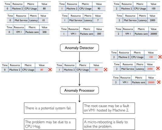
Figure 3.1 illustrates the overall DyFAULT dataflow. DyFAULT periodically collects system runtime metric data. The tables in Figure 3.1 are an excerpt of the collected metrics that include CPU usage percentage on Machine 2, network latency in the mail service, and number of packets sent on Virtual Machine 1. DyFAULT’s Anomaly Detector analyzes the runtime metric data. In the example of Figure 3.1, at time 0, the Anomaly Detector observes that the value of CPU usage percentage on Machine 2 goes beyond 90, which deviates from its normal range in the past, thus regard it as an anomaly(marked in red in the table). At time 2, the Anomaly Detector finds three anomalies.

A single deviation of a value can be just a false alarm. In this example, at time 0, the anomaly <Machine 2, CPU Usage, 80> may come from a temporary system check that consume a significant CPU resource in a very short time, which will not result in a failure. Therefore, the outcomes of the Anomaly Detector is not evident enough for a prediction or localization.

DyFAULT’s Anomaly Processor refines and analyzes the anomalies, taking into account the interactions between the metrics. In Figure 3.1, at 0, the Anomaly Processor consider a single anomaly not significant enough to lead to a potential failure. While at time 2, the three anomalies indicate a propagation of errors among the metrics. The Anomaly Processor generates a failure alert and infers that the fault is most likely a CPU hog on Virtual Machine 1 hosted on Machine 2.

In my thesis I focus on the design and implementation of DyFAULT to producing failure alert, fault type and location.

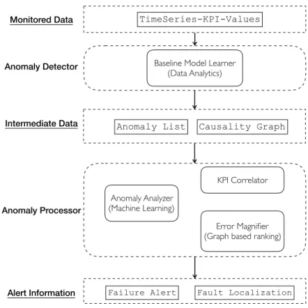
3.2 Framework Overview

Figure 3.2 shows the main components of DyFAULT: monitored data, anomaly detector, interme-diate data, anomaly processor, alert information.

(30)

16 3.2 Framework Overview

There is a potential system fail. The root cause may be a fault _{on VM1 hosted by Machine 2.} The problem may be due to a

CPU Hog. A micro-rebooting is likely to solve the problem.

Time Resource Metric Value

0 Machine 2 CPU Usage 80

0 Mail Service Latency 10

0 VM 1 Packets sent 200

Anomaly Detector

Anomaly Processor

Figure 3.1. The DyFAULT freamework

3.2.1 Monitored Data

The Monitored Data are Key Performance Indicators, KPI, that is, < resource, met rics > pairs. For instance, a KPI can be the CPU Usage of a specific virtual machine, or the service latency of a specific application. A KPI specifies a measurable unit of the running system.

At runtime, DyFAULT monitors KPI data from the system. At different timestamp, a KPI may have different values. The input of DyFAULT is a series of “KPI-Value” tuples (as shown in Figure 3.1).

DyFAULT uses input data to train models (training data) that DyFAULT uses to predict failures on new input data (operational data).

3.2.2 Anomaly Detector

The DyFAULT Anomaly Detector processes the monitored data at training time to build models and at operational time to detect anomalies.

The DyFAULT Anomaly Detector (i) identifies anomalous values, (ii) detects correlations between KPIs, and (iii) produces a graph data structure to represent the pairwise correlations for further analysis.

The Anomaly Detector is composed of a Baseline Model Learner that analyzes historical data, involving Data Analytics technique, such as statistical inference, to generate the Intermediate

(31)

17 3.2 Framework Overview

Baseline Model Learner (Data Analytics)

Anomaly Analyzer (Machine Learning)

KPI Correlator

Error Magnifier (Graph based ranking) Anomaly Detector Anomaly Processor Failure Alert Intermediate Data Fault Localization Anomaly List TimeSeries-KPI-Values Monitored Data Alert Information Causality Graph

Figure 3.2. Overall design

Data.

3.2.3 Intermediate Data

The Anomaly Detector produces Intermediate Data that include an Anomaly List and a Causality Graph.

The Anomaly List is a list of anomalous KPIs values at a given timestamp.

The Causality Graph is a graph that models the correlation between KPIs. Each vertex of the Causality Graph represents a KPI, and the weights of the edges indicate the correlation significance between the KPIs that correspond to the nodes.

DyFAULT uses the Anomaly List as the regular input of the Anomaly Processor, and the Causality Graph as shared knowledge that the Anomaly Processor uses on demand.

3.2.4 Anomaly Processor

The Anomaly Processor refines the intermediate data, and is composed of an Anomaly Analyzer , a KPI Correlator and an Error Magnifier .

The Anomaly Analyzer analyzes the anomaly list. The anomaly list is a vector of boolean values that indicate the KPIs with anomalous values at the given timestamp. The Anomaly

(32)

18 3.3 Execution based workflow

Analyzer deals with the Anomaly List as a classification problems given vector-like inputs. The KPI Correlator and Error Magnifier combine the Anomaly List and the Causality Graph for further analysis. The KPI Correlator marks anomalous KPIs in the Causality Graph, and removes the KPIs with normal valuers to produce a graph of anomalous KPIs. The Error Magnifier implements different graph-based ranking algorithms to rank the significance of the anomalous KPIs and infer likely root cause of the fault.

3.2.5 Alert Information

DyFAULT coordinates the components in the Anomaly Processor, to issue Alert Informations that include: (i) an alert prediction: a boolean value that indicates if the monitored KPIs values suggests a potential failure’ (ii) an alert type: the type of fault that will lead to the failure, for example a memory leak. (iii) an alert location: the subset of resources where the fault is most likely located.

An alert prediction constitutes a Failure Alert, and alert type and an alert location comprise a Fault Localization.

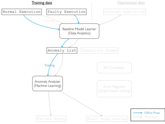
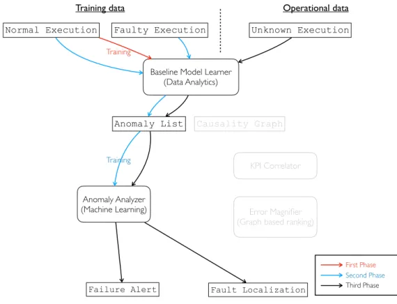
3.3 Execution based workflow

DyFAULT implements two main workflows, PreMiSE and LOUD, depending on the available training data that can be Normal execution data that are collected during normal executions, and Faulty execution data that are collected in the presence of active faults that lead to failures. While Normal execution data can be monitored on all target systems, collecting a useful amount of Faulty execution data requires intensive fault seeding that may not be always allowed, depending on the target applications.

PreMiSE requires both normal and faulty execution data, and process the training data in two stages to build the model, while LOUD trains models with normal training data only.

PreMiSE and LOUD share the anomaly detector component, but differ in the anomaly proces-sor components, due to the different intermediate data that PreMiSE produces with both normal and faulty execution data, while LOUD produces with normal execution data only.

3.3.1 PreMiSE

Figure 3.3 indicates the PreMiSE workflow. The red and blue lines indicate the training workflow, while the black lines indicate the operational workflow.

PreMiSE iterates the model training twice, with normal execution data first and with faulty execution data later. PreMiSE trains the Baseline Model Learner with Normal Execution data, the red line in Figure 3.3, to build a model of normal behavior, and use the faulty execution data, the blue lines in Figure 3.3, to update the model with information about anomalies and failures. At operational time PreMiSE executes the Baseline Model Learner with the model built with the first stage training to produce an Anomaly List, and executes the Anomaly Analyzer with the model trained from the second stage training to produce fault information, the black lines in the figure.

(33)

19 3.4 Summary

KPI Correlator

Error Magnifier (Graph based ranking)

Failure Alert Fault Localization

Normal Execution

Training

Faulty Execution

Training

Anomaly List

Training data Operational data Unknown Execution

First Phase Second Phase Third Phase

Causality Graph

Figure 3.3. PreMiSE workflow

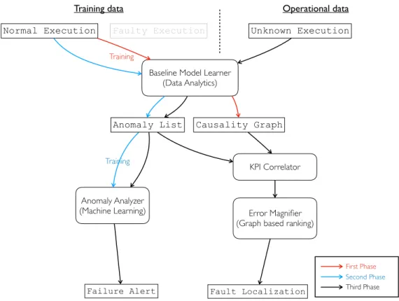
3.3.2 LOUD

Figure 3.4 shows the LOUD workflow. LOUD trains the models with normal execution data only, and proceeds in two training stages.

LOUD shares the first training stage with PreMiSE, as the Baseline Model Learner building the same model with KPI values collected only during normal execution. The LOUD anomaly list does not encode data about faulty executions, and the LOUD anomaly analyzer can predict failures, but not identify the fault type and location.

The LOUD KPI Correlator and Error Magnifier use the causality graph to rank the anomalies in the anomaly list according to their mutual correlations, to locate faults. The LOUD KPI Corre-lator prunes uncorrelated anomalies from the causality graph, while the Error Magnifier ranks KPIs according to the weighted connections in the pruned causality graph. LOUD identifies as possible fault location the resources of the highly ranked KPIs.

3.4 Summary

Current self-healing techniques do not cope with the complexity of data analysis of metric data of large multi-tier systems, complexity that is due to a large amount of KPIs and a high dynamics of value range for each KPI.

(34)

20 3.4 Summary

KPI Correlator

Normal Execution

Training

Faulty Execution

Training

Anomaly List

Training data Operational data Unknown Execution

First Phase Second Phase Third Phase

Causality Graph

Figure 3.4. LOUD workflow

DyFAULT reduce the high dimension of raw input KPI data by separating failure prediction and fault localization into two stages, to reduce the high dimension of raw input KPI data. The first stage focuses on single KPIs, and transform the corresponding data from concrete numeric value to discrete binary value that indicates whether or not a single KPI is normal. The second stage aggregates all KPIs and consider their interaction to produce failure prediction and fault localization, benefiting from the dimension reduction by the first stage, the second stage deals with reasonable complexity in the data.

(35)

Chapter 4

Anomaly Detection

In this chapter, I present the design and implementation of the Baseline Model Learner component, the component that PreMiSE and LOUD share to detect anomalies.

The Baseline Model Learner works in two stages, training and operational. At training time, Baseline Model Learner leverages KPIs values monitored during normal execution to learn a baseline model that captures the normal range of value for each KPI, and to produce a Causality Graph that captures the correlation between KPIs. At operational time, Baseline Model Learner analyzes KPI values with the trained model to detect anomalies. Baseline Model Learner groups KPIs with anomalous values at the same time into Anomaly List. The Anomaly List and Causality Graph form the intermediate data for further analysis.

Section 4.1 discusses the training of the Baseline Model Learner by presenting how the Baseline Model Learner samples data from the running system, and builds a model from the data sampled during normal execution. Section 4.2 describes the online operational phase of the Baseline Model Learner by discussing how the Baseline Model Learner detect anomalous KPI with the model.

4.1 Training

As shown in Figure 4.1, in the training phase, the Baseline Model Learner (i) monitors KPI data under normal execution of the system, (ii) builds a Baseline Model with the monitored data, and (iii) derives a Causality Graph that represents the causality relationship between KPIs.

4.1.1 KPI monitoring

DyFAULT elaborates KPI values periodically sampled with probes at different locations and at multiple layers in the system.

System administrators can use different probes, for instance general data collection tools [22], or application specific monitoring services [123]. Administrators can also configured the data sampling rate in their implementation according to requirement difference. In our experiments we collected over 600 KPIs of over 90 types, as discussed in Chapter 7.

DyFAULT elaborates KPI values on an independent machine, thus limiting the overhead on the target cloud system to the probes that impact on host machine’s resource only with monitored data query and network communication, with negligible costs.

(36)

22 4.1 Training

KPI Correlator

Normal Execution Training

Faulty Execution

Training

Anomaly List

Training data Operational data

Unknown Execution

Offline Phase

Online Phase

Causality Graph

Figure 4.1. Oﬄine Training of Baseline Model Learner

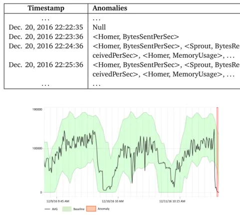
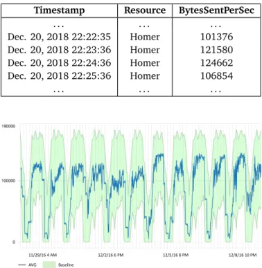
Table 4.1 presents a sample set of input data. Input data are time series data in the form of streams ordered by time. In the table, the specific KPI is hHomer, B y tesSentPerSeci. Homer is one of the virtual machines that we use in our experiments, a standard XML Document Management Server that stores MMTEL (MultiMedia TELephony) service settings of the users (see Chapter 7). BytesSentPerSec reports the outgoing number of bytes per second in the network communication. As the timestamp (first column) changes, sampled values(third column) also changes.

4.1.2 Baseline Model Learner

The Baseline Model Learner analyzes time series KPI data and derives the Baseline Model that models the behavior of the system under normal execution conditions. For each KPI, the model includes descriptive metrics of the historical data, such as mean value, maximum and minimum values, seasonality and seasonal offsets [10].

The Baseline Model Learner trains the models with raw data collected from KPI monitoring during a normal execution, and derives descriptive metrics from the input data with statistical test. The portability of the Baseline Model Learner relies on the flexibility of the approach: many algorithms that reads KPI data from the system and produces a model to judge whether an input is normal or not can be valid implementations of the detector. of Baseline Model Learner .

Figure 4.2 shows a baseline model of the KPI hHomer, B y tesSentPerSeci, as we discussed in the example in Section 4.1.1. The green area in the figure marks the range of values that the Baseline Model considers as normal as the Baseline Model Learner infers from the input data.

Baseline Model Learner infers also KPI correlation and models them in the form of a Causality Graph, For each pair of KPIs, Baseline Model Learner utilizes Granger causality tests [3] to mine

(37)

23 4.1 Training

Table 4.1. Sample time series for KPI BytesSentPerSec collected at node Homer

Timestamp Resource BytesSentPerSec

. . . . Dec. 20, 2018 22:22:35 Homer 101376 Dec. 20, 2018 22:23:36 Homer 121580 Dec. 20, 2018 22:24:36 Homer 124662 Dec. 20, 2018 22:25:36 Homer 106854 . . . .

11/29/16&4&AM 12/2/16&6 PM 12/5/16&8 PM 12/8/16&10&PM AVG Baseline

Figure 4.2. Sample baseline model of single KPI: BytesSentPerSec for Homer virtual machine

the impact between KPIs. A time series x is a Granger cause of a time series y, if and only if the regression analysis of y based on past values of both y and x is statistically more accurate than the regression analysis of y based on past values of y only.

Figure 4.3. A sample baseline model: an excerpt from a Granger causality graph

Baseline Model Learner integrates the pairwise causality relationships and represents them as a graph, the Causality Graph. In the Causality Graph, vertexes correspond to KPIs and weighted edges indicate the significance of the causality relationship. The Causality Graph both assists the Baseline Model Learner in deriving the Baseline Model, and serves as a extra information in

(38)

24 4.2 Detecting Anomalies at Operational Time

fault localization, which we will discuss in Chapter 6.

Figure 4.3 shows an excerpt of a Granger Causality Graph. The vertexes correspond to KPIs, and the weights of the edges, ranging in the interval [0, 1], indicate the significance of the causal relationship. For example in the figure, the KPI BytesReceivedPerSec in Homer has is strongly correlated with Sscpuidle in Homer.

KPI Correlator

Normal Execution Training

Faulty Execution

Training

Anomaly List

Training data Operational data

Unknown Execution

Offline Phase

Online Phase

Causality Graph

Figure 4.4. The operational time detection workflow of Baseline Model Learner

4.2 Detecting Anomalies at Operational Time

At operational time, Baseline Model Learner collects KPI monitored data, and uses the Baseline Model to identify anomalous KPIs (anomalies).

Figure 4.4 illustrates the workflow of the detection at operational time.

The Baseline Model Learner detects univariate anomalies as samples out of range, as shown in Figure 4.5. Given an observed value yt of a time series y at time t, and the corresponding expected value ˆyt in y, yt is anomalous if the variance ˆ2( yt, ˆyt) is above an inferred threshold.

For each individual KPI, Baseline Model Learner performs the same analysis. Thus, at a given timestamp, Baseline Model Learner produces a list, which contains the KPIs that it detects as anomalous. Table 4.2 shows a sample of the anomaly list.

4.3 Summary

The Baseline Model Learner is the mounting point where DyFAULT gets the status of the monitored system’s runtime and perform the initial analysis. DyFAULT uses system metrics in the form of time series data as its input, due to its lightweightness and portability.

(39)

25 4.3 Summary

Table 4.2. Sample the Anomaly List

Timestamp Anomalies

. . . .

Dec. 20, 2016 22:22:35 Null

Dec. 20, 2016 22:23:36 _{<Homer, BytesSentPerSec>}

Dec. 20, 2016 22:24:36 _{<Homer, BytesSentPerSec>, <Sprout,} BytesRe-ceivedPerSec>, <Homer, MemoryUsage>, . . . Dec. 20, 2016 22:25:36 _{<Homer, BytesSentPerSec>, <Sprout,}

BytesRe-ceivedPerSec>, <Homer, MemoryUsage>, . . .

. . . .

12/9/16&9:45&AM 12/10/16&10&AM 12/11/16&10:15&AM AVG Baseline Anomaly

Figure 4.5. A sample univariate anomalous behavior

Because of the large number of system KPIs that a multi-tier system can provide in reality, it is challenging to build a unified model that is complicated enough to capture the variance of concrete numeric values of all KPIs. As covered by Section 4.1, for each KPI, DyFAULT , builds a single model that describes the normal statistic metrics of its value.

As covered by Section 4.2, at each timestamp during operational time, Baseline Model Learner reports each KPI as either normal or anomalous. A single anomalous KPI is not sufficient to reveal a potential failure in a large multi-tier system due to its complexity, thus further data processing is needed.

The set of anomalous KPIs, namely anomalies, along with the Causality Graph that models the correlation between KPIs, are the outcome of Baseline Model Learner and are used by PreMiSE and LOUD.

(40)