Full-Scale Fire Tests to Validate NRC's Fire Growth Model - Open Office Arrangement

Publisher’s version / Version de l'éditeur:

Vous avez des questions? Nous pouvons vous aider. Pour communiquer directement avec un auteur, consultez la première page de la revue dans laquelle son article a été publié afin de trouver ses coordonnées. Si vous n’arrivez pas à les repérer, communiquez avec nous à PublicationsArchive-ArchivesPublications@nrc-cnrc.gc.ca.

Questions? Contact the NRC Publications Archive team at

PublicationsArchive-ArchivesPublications@nrc-cnrc.gc.ca. If you wish to email the authors directly, please see the first page of the publication for their contact information.

https://publications-cnrc.canada.ca/fra/droits

L’accès à ce site Web et l’utilisation de son contenu sont assujettis aux conditions présentées dans le site LISEZ CES CONDITIONS ATTENTIVEMENT AVANT D’UTILISER CE SITE WEB.

Internal Report (National Research Council of Canada. Institute for Research in Construction), 1996-06-01

READ THESE TERMS AND CONDITIONS CAREFULLY BEFORE USING THIS WEBSITE.

https://nrc-publications.canada.ca/eng/copyright

NRC Publications Archive Record / Notice des Archives des publications du CNRC :

https://nrc-publications.canada.ca/eng/view/object/?id=f93789f4-3601-45e4-b6e4-17de6eb00895 https://publications-cnrc.canada.ca/fra/voir/objet/?id=f93789f4-3601-45e4-b6e4-17de6eb00895

NRC Publications Archive

Archives des publications du CNRC

For the publisher’s version, please access the DOI link below./ Pour consulter la version de l’éditeur, utilisez le lien DOI ci-dessous.

https://doi.org/10.4224/20338252

Access and use of this website and the material on it are subject to the Terms and Conditions set forth at

Full-Scale Fire Tests to Validate NRC's Fire Growth Model - Open Office Arrangement

-- Ser TH1 R427 no. 717 c. 2 BLDG

.

Netlonal Rerrarch Coneell national

I$11

Councll Canada de recherche8 Canada

Full4Scale Fire Tests to Validate

NRC's

Fire Growth Model

-

Open Office Arrangement

n a l r e p o r t ( ~ n s t l t u t e t

I ALYSE

I

'3

by Bavld Yung and Jennifer Ryan Internal Report No. 71 7

Date,

of

Issue: June 1996

CISTLIICI Y'P NRC/CNRC' IXC Ser

X e c e ~ v e c l o n : 0 7 l b - 9 6

FULL-SCALE FIRE TESTS TO VALIDATE NRC'S

FIRE GROWTH MODEL - OPEN OFFICE ARRANGEMENT

David Yung and Jennifer Ryan

ABSTRACT

The objectives of these tests were to determine whether a simple fuel geometry can conservatively represent real furniture for fire risk assessment and to verify NRC's fire growth submodel for office buildings. The tests were conducted using both office

furniture and wood cribs and measured the temperature, heat release rate, mass flow rate and concentrations of combustion gases. This was done using an open office arrangement. The results are compared to determine how well wood cribs conservatively represented typical ofice furniture. The results will be used later to validate the F i R E C W fire growth submodel which uses wood cribs as the representative fuel.

FULL-SCALE FIRE TESTS TO VALIDATE NRC'S

FIRE GROWTH MODEL - OPEN OFFICE ARRANGEMENT

by

David Yung and Jennifer Ryan

INTRODUCTION

The National Research Council of Canada (NRC) is presently developing a risk- cost assessment model called F i R E C W (Fire Risk Evaluation and Cost Assessment Model). FiRECAMTM predicts the overall fire safety performance in a building.

Currently, the model

is

suitable for application to apartment and office buildings. This model is dependent on submodels that predict fire growth and spread, smoke movement, occupant response and evacuation and fire department response and effectiveness.

For fire risk assessment, it is necessary to predict the fire growth characteristics of various fires such as smouldering fires, flaming non-flashover fires and flashover fires. Predicting fire growth can be difficult due to the varying types, amounts and arrangements of combustibles in a room. To make it simple, the fire growth suhmodel was developed using represcntative fuels. Polyurethane foam slabs were used as the representative fuel for residential furniture and wood cribs were used for office furniture.

The fire growth submodel predicts the burning rate, room temperature and

production and

concentration

of smokc and toxic gas& as a function of time. Thc output of the tire growth submodel is used bv other submodels in F i R E C W to calculate the risk-to-life70 the occupants in a buil&ng.

To validate the fire growth submodel for office buildings, full-scale fire tests were performed to simulate fires in an office situation. In particular, these tests were conducted for Public Works and Government Services Canada (PWGSC) using an open office arrangement.

The tests were conducted using both typical office furniture and wood cribs to determine how well wood cribs conservatively represented typical office furniture. The results will be used later to validate the fire growth submodel which uses wood cribs as the representative fuel.

EXPERIMENTAL SETUP

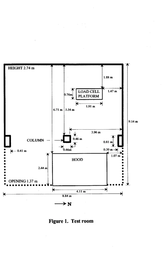
All of the tests were conducted in an 8.84 x 9.14 x 2.74 m high test room.

Figure 1 is a schematic of the test room. At the east end of the room, along the 8.84 m wall and partially along the two 9.14 m walls, there was an opening of 1.37 m in height.

In the ceiling, there was a stainless steel hood, measuring 2.44 x 4.15 m, attached to a 0.55 m diameter galvanized duct. The duct is 13.2 m long and was used to exhaust the

fire gases, using a fan at the end of the duct, to the outside of the bum hall.

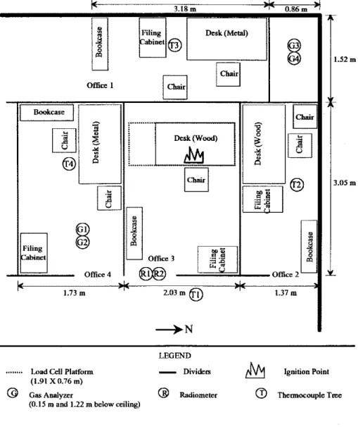
Open Ofice Furniture

A schematic of the furniture arrangement is shown in Figure 2. The open office setup consisted of four work spaces, separated by 1.4 m high dividers. Each office contained a desk, 2 chairs, a bookcase and a filing cabinet except for Office 3 which only had

1

chair. In two of the officcs (Offices 1 and 4), the desks were metal and, in the other two (Offices

2

and 3). thcy were wood.

The approximate sizes of furniture used for the office tests were as follows: desks

-

1.52 x 0.76 x 0.76 rqchairs

-

0.41 x 0.41 m, bookcases

-

0.91 x 0.30 x 1.22 m, and filing cabinets

-

0.46 x 0.7 x 0.76 m (Offices 1 and 4) and 0.46 x 0.7 x 1.29 m (Offices 2 and 3).

The offices also contained books and papers. In Offices 1 and 4,9.9 kg of papers and books were spread on the desks. In Office 2, 19.8 kg of papers and books were spread on the desk. As well as 19.8 kg of papers and books on the desk, Office 3 also had a computer monitor and keyboard. In addition, two 9.9 kg boxes of paper were put under the desk as the initial burning object.

The amount and type of furniture representative of a typical office was determined by studying various open and closed concept offices. A schematic was then constructed of the furniture arrangement that was representative of a typical open office. The furniture required for the tests was provided by PWGSC.

Wood Cribs As Representative Fuel

The wood cribs used as the representative fuel for the tests, measured 0.61 x 0.61 x 0.41 m high and weighed between 17 and 18 kg. They were constructed from nominal 25.4 x 50.8 mm wood sticks. Each wood crib had 10 x 10 x 5 sticks.

To determine how many wood cribs were required t:, represent the office furniture, it was assumed that, on average, an office contains 25 kg/m of furniture. From this, the maximum number of wood cribs was determined. Since only a percentage of furniture in an office is combustible, only a Fraction of the maximum number of wood cribs was required. Based on the furniture used for the other tests, it was assumed that half of the furniture in the room was combustible.

For the test with wood cribs, Table 2 indicates the number of wood cribs used to represent the furniture in each office.

The wood cribs were positioned side by side in Offices 1,2 and 4 and on top of each other in Office 3. A schematic of the arrangement is shown in Figure 3.

The wood cribs were ignited using 300 mL of methyl hydrate which was placed, in a pan, under the four wood cribs in Office 3. The total weight of the wood cribs in

Office 3 was 69.3 kg.

Instrumentation

Temperature

The gas temperature in the tcst room and the duct was measured using

thermocouples. 'l'hcrmocouplc trecs wcrc uscd to dctcrminc thc vertical gas tcmpcraturc protilc in thc tcst room. The thermocouples used wcrc Chromcl-Alumcl ("K" typc).

The instrumentation for the open office setup required four thermocouple trees (TI, T2, T3 and T4). Each tree was 2.74 m high and had eight thermocouples that were approximately 36 cm apart. The first thermocouple was 5.08 cm below the ceiling. See Figure 4 for the vcrtical placement of the thermocouples. Two thermocouples were also located in the duct near the pitot tubc.

Gas Concentration

To determine the concentrations of combustion gases, Beckman infrared gas analyzers were used. The combustion gases analyzed were oxygen, carbon monoxide and carbon dioxide. The sampling train started with a sampling tube that took a representative gas sample. Samples were taken from both the room and the duct. In the duct the

sampling tube was at a position, about 8.3 m from the entrance of the exhaust duct, to ensure that the products were uniformly mixed. The gases then passed through a cold trap to condcnsc any water vapour, The watcr was then rcmovcd by passing the gases through a desiccant containing Drierite (pellets of anhydrous calcium sulfate). The gases then went though a pump &d into a flow regulatorthat reduced the flow into the analyzers to 1 to 1.5 Wmin. Any excess flow was discharged.

The gas analyzers used four sampling tubes in the test room (GI, G2, G3 and G4) and one in the duct. Tubes 1 and 2 were located 1.76 m from the column. Tube 1 (Gl) was 0.15 m below the ceiling and Tube 2 (G2) was 1.23 m below the ceiling. Tubes 3 and 4 were located 0.46 m from the northwest comer of the test room. Tube 3 (G3) was 0.15 m below the ceiling and Tube 4 (G4) was 1.23 m below the ceiling. Carbon dioxide measurements were taken from GI, G2, G3 and the exhaust duct for the furniture test and G2, G3, G4 and the exhaust duct for the wood crib test. Carbon monoxide measurements were taken from GI, G2, G3, G4 and the exhaust duct. Oxygen measurements were taken only in the exhaust duct.

Heat Flux

The heat flux in the test r F m was measured using*heat flux meters. Two types of meters were used, a Gardon Gage and a Schmidt-Boelter

.

Neither of the meters

contained a window so they were configured as total heat flux meters.

Two radiometers (R1 and R2) were used for this setup. They were located southwest of TI at the entrance to Office 3.

Mass Loss

The mass loss was determined using a load cell platform. The platform was attached to four 1000 pound load cells.

The load cell platform was located 1.88 m from the west wall and 1.47 m from the north wall.

Mass Flow Rates

The mass flpw rate was determined using the pressure drop and the temperature in the duct. A Dwyer pitot tube measured the pressure drop in the duct.

For a schematic of the instrumentation setup see Figure 5.

' Cenain commcruial products dre ident~fied in this paper in order to adequately specify the experimental procalure. In no caw docs such identific;rtion imply recommendations or ~ndorsment by the Nat~onal Research Council nor doc.; 11 imply that the product or material identified is the b~.st availablc for rhc

RESULTS

The location of the experimental data from each test and its transformation is explained in Table 3. The

*

in the file name is the date that the test was performed, i.e., nv29.

Graphs A1 through L1 were produced from the *dat.spw file. The file names for the graphs are located at the bottom right hand comer of the graph.

Calculations to determine the upper and lower limits of the heat flow rate, mass flow rate, CO and COz concentrations out of the room were also performed. The equations used for these calculations are located in Appendix A - Equations. The transforms tabulated in Table 4 were used to perform these calculations.

Open Office Furniture Test

For the open office tests, the variables in the equations used to determine the upper and lower limits for the heat flow rate, mass flow rate, and CO and CO* concentrations at the door had to be modified. The equations are derived for room fires where the fire is enclosed and vented through a room opening. The open office anangement had no enclosure. Thus, there will be an increase in the amount of heat lost. To account for this additional loss of heat, the area (A) in the heat loss equation (Qwm,) was increased by 50%. Originally, the room size was considered to be the total area of the four of2ces (23.45 m2). When the area was increased by 50% the room size became 35.19 m ,which is equivalent to an area with a radius of 3.35 m. Since the ceiling was 2.74 m high, the

heatdissipation-radiusheight

ratio is 1.2 which is not unreasonable. In determining the mass flow rate limits, the temperature at the ceiling of Thermocouple Tree 1 (TI) was used as the temperature at the door ( T h ) since there was no door.

A summary of the channels and data measured by the data acquisition system during the burning of furniture in the open office setup can he found in Table 5. The graphs that were produced from the experimental data are summarized in Table 6.

The furniture test was terminated after 11.5 minutes to prevent damage to the test room and the cxhaust duct.

Open Office Wood Crib Test

The modifications to the equations for the upper and lower limits of the heat flow rate and mass flow rate used for the open office furniture test were also used in the calculations performed for the open office wood crib test.

A summary of the channels and data measured by the data acquisition system during the burning of wood cribs in the open office setup can be found in Table 7. The graphs that were produced from the experimental data are summarized in Table 8.

The wood crib test was terminated after 7.8 minutes to prevent damage to the test room and the exhaust duct.

Comparison of fire characteristics of wood cribs and real furniture

A comparison of thc results from the two tcsts is shown in Figures 8 through 13. To prevent damagc to the test room and the cxhaust duct, the tests had to be terminated at

different times. The furniture test was terminated after 11.5 minutes and the wood crib test was terminated after 7.8 minutes.

The results in Figure 8 show that the average temperature increase for the furniture test was gradual, whereas for the wood crib test it was more rapid. For the furniture test, the temperature was 68'C after seven minutes, whereas for the wood crib test, the

temperature was 128°C. In Figures 9 and 10, the average concentrations of carbon monoxide and carbon dioxide in the test room were plotted. For both of these gases, the increase in concentration was comparable between the wood cribs and real furniture. Figure 11 indicates that the increase in heat release rate was more rapid for the wood cribs. The comparison of mass flow rate variations in the exhaust duct in Figure 12

shows that they are about the same for the two tests, however the decrease occurs sooner with the wood crib test. Figure 13 compares the upper and lower limits of the mass flow rate at the door. From this it can be seen that the wood crib test gave lower values than the furniture test. This is a result of the wood crib test having a much hotter fire than the furniture test, therefore a decrease in the density of the combustion gases and a decrease in the mass flow rate out of the room. For conservative modeling of fire severity the upper limits of the mass flow rate should be used. Figure 13 shows that the upper limits from both of the tests were fairly close.

The results show that the wood cribs produced a slightly more severe fire than the furniture did. Therefore, the results indicate that wood cribs could be used to

conservatively represent real furniture. Acknowledgments

The authors would like to thank Public Works and Government Services Canada (PWGSC) for partial funding support to this study and for providing the office furniture for the fire experiments (Contract A4412). The authors would also like to thank Mr. Don Carpenter for his help in conducting the experiments.

Table 1. Determination of the wood cribs required to represent the furniture

* _{Assuming that the mass per unit area is 25 kg/m}

_.

**

Where each crib weighs 18 kg.

Table 2. Number of wood cribs per room for the open office tests Number of

Number Wood Cribs

Office 1 Office 2

Office 3 Oftice 4

Table 3. Fies containing the experimental data

&&: The transforms mentioned are located in Appendix B - SigmaPlot Transforms. File name

*.prn *.spw *dat.spw

Table 4. Transforms used to determine upper and lower limits at the door Description

the experimental data obtained from the data acquisition system

*.pm imported into Sigmaplot

*.spw transformed using *data.xfm (converts data to desirable format, i.e., pressure to Pa), *fow.xfm (calculates the volumetric and mass flow rates in the duct), and *hrr.xfm (calculates the heat release rate)

File name *heat.xfm *mass.xfm *co.xfm *coZ.xfm Description

calculates the upper and lower limits of the heat flow rate calculates the upper and lower limits of the mass flow rate calculates the upper and lower limits of the CO concentration calculates the upper and lower limits of the C02 concentration

7

Table

5

Map of the data acquisition system for the open office furniture test (Cont.)

9

LEGEND

.,...

Load Cclf Platform

-

Divide=

&

Ignition Poiot (1.91 X0.76 m)

@

Car Aoalyvr

@

Radiometer @ Thermocouple Tnc

(0.15 m and 1.22 m below ceiling)

Office 1

I

l I

LEGEND

... b a d Cell Platform

-

Dividers

&

Ignition Point

0

Wood Crib (1.91 X 0.76"~) (0.61X0.61 X0.41 n

@

Gas Analylrr

@

Radiometer

@

Thermocouple Tme (0.15 m and 1.22 mbelow ceiling)

Figure 3. Wood crib arrangement for open office tests

Cciling 2.74 m 6 7 R 7 Floor

F

LEGEND

@

Gas Analyzer

@

RadiomcCr

@

Thsrmocoupls TEE

(0.15 m and 1.22 m b l o w ceiling)

1.52, -1-

.I#

2.74 m >

Figure 5. Instrumentation for the open office tests (0.46 X 0.46 m) ,. 2.62 m

":

0.48 m 7r 2.92 m

*

1.93 m

l7

0 . 4 m] Load Cell Platform

(1.91 X0.76 m)

1.17 m

0

4.09 m >

Appendii A

Equations

The following equations were obtained from the NFL internal document

"Equations and Calculations for the Heat Release Rate and Mass Flow Rate Through the ASHRAE Test Room Exhaust Duct" written by Peter Richardson (Februa~y, 1996).

1) Velocity

where

v, velocity of exhaust through the exhaust duct, corrected to 20°C ( d s )

T

temperature in the exhaust duct (K)

AF'

pressure difference in the exhaust duct recorded with pitot tube (Pa)

2) Volumetric flow rate

where

VE volumetric flow rate through the exhaust duct, corrected to 20°C (m3/s)

k, shape factor

$

velocity through the exhaust duct, correctet to 20°C (mls) cross sectional area of the exhaust duct (m )

3) Mass flow rate

where

m, mass flow rate through the exhaust duct, corrected to 20°C (kgls)

p air density at 20°C, 1.2135 (kg/mm)

YE volumetric flow rate through the exhaust duct, corrected to 20°C (m3/s)

Pg barometric pressure (Pa)

T temperature in the cxhaust duct (K)

4)

Heat release rate

with $ given by

where

QHRR heat release rate

(kW)

E heat release per volume of oxygen consumed, 17400 &l/m3)

0

oxygen depletion factor

O;

initial oxygen concentration

V, volumetric flow rate through the exhaust duct, corrected to 20°C (m3/s)

U; oxygen concentration recorded in the exhaust duct

CO' carbon monoxide concentration recorded in the exhaust duct

CU; carbon dioxide concentration recorded in the exhaust duct

5) Heat flow rate at the door

with Q,, given by

Q/ms = Q,,,dj&" + Qrn"-.,iO"

Qlwcmm) = GA

(q4

-

q4)

+

hA

(T,

-

T , )

with h = 2.49(~, -

T,)'."

where

A area of the room (mZ)

Q heat flow rate (W)

T,

ambient temperature (K)

T, ceiling temperature (K)

0 Stefan-Boltzrnann constant 5.67x10-~ (W/m .K 2 4 )

where

Cp specific heat (M/kg."C)

tn mass flow rate (kgls)

T,

ambient temperature

("C)

Tdoor temperature at the door ("C)

7)

Gas concentration at the door

-

Xdoormdoor - Xducrmdvcr

where

x concentration of carbon monoxide or carbon dioxide (%)

Appendix B

Sigmaplot Transforms Test: Open Office

-

Furniture

;File: nv29dataxfm

;Converts the data to a desirable format.

;NOTE: This transform has to be

run

on the raw data first. The rest of the transforms can ;then be run.

;Analyzer ranges

R02 = 25

;a

range in the duct (%)

RC02 = 5 ;COz range in the duct (%)

RCO = 1 ;CO range in the duct (%)

RCOM = I ;CO range in the room (%)

RCO2M= 5 ;C@ range in the room (%)

;Conversions

col(5) = col(5)

*

1000 ;duct pressure (Pa)

col(7) = col(7)

*

R c o

*

10 $0 concentration (%)

coI(8) = col(8)

*

R02

*

10 ;02 concentration (%) col(l1) = col(1 I)

*

RCOM *I0 ;CO concentration (%) col(12) = col(12)

*

RCOM

*

10 ;CO concentration (%) col(13) = col(13)

*

RCOM

*

10 ;CO concentration (Oh) col(15) = col(15)

*

- RC02M

*

10 ;C02 concentration (%) coI(16) = col(16)

*

RCO2M

*

10 ;C02 concentration (%)

col(17) = col(17)

*

1 / 20 ;CO concentration (Oh) siemens col(l8) = col(18)

*

-

4 / 20 ;C02 concentration (%) siemens col(19) = ((col(19) - 4) 1 1600)

*

100 ;CO concentration (%, scale 0% - 1%) col(20) = ((col(20) - 4) 1 160)

*

100 ;COZ concentration (%, scale 0% - 10%)

col(49) = col(49)

*

1000 ;room pressure (Pa)

col(50) = col(50)

*

1000 ;room pressure (Pa)

col(5 1) = col(5 1)

*

1000 ;room pressure (Pa)

col(60) = col(60) / 60 ;time (min)

;Calculate mass loss

col(59) = col(59)

*

( - 10) ;mass (Ib)

im = 277.9 ;initial mass (lb)

col(59) = im

-

col(59) ;mass loss (Ib)

col(59) = coI(59) / 2.2 ;mass loss (kg)

;Calculates the heat flux in kw/m2.

;Two types of radiometers were used, a Gardon Gage and a Schmidt-Boelter. ;Columns Gardon = col(79) Schmidt = col(80) . . ;Constants mg = 1.96 ms = 2.23 C = 11.3565 Qg = Gardon / mg coI(79) = (Qg

*

c )

*

1000 Qs = Schmidt /

rns

col(80) = (Qs

*

c )

* 1000

;transducer output in mV (Gardon) ;transducer output in mV (Schmidt) ;slope from calibration curve (Gardon) ;slope from calibration curve (Schmi$t) ;conversion from ~tu/ft'sec to kW/m ;heat flux (Btu/f$ec, Gardon) ;heat flux @W/m

,

Gardon) ;heat flux (Btu/f$ec, Schmidt) ;heat flux (kW/m

,

Schmidt)

;File: nv29fow.xfm

;Calculates the mass flow rate though the duct in kg/s ;Calculate velocity in duct

T = col(9) +273.15 ;exhaust duct temperature (K)

P = col(5) ;pressure from pitot tube (Pa)

vs = 1.291

*

sqrt(T

*

P / 293)

*

293 / T ;velocity in duct ( d s ) ;Calculate volumetric flow rate

r = 0.279 pi = 3.1415927 kc = 0.91 A = p i * r A 2 V E = k c * v s * A col(81) = VE

;Calculate air density PB = 102400

rho = PB / (288

*

293) ;Calculate mass flow rate mE=rho*VE

col(82) =

mE

;File: nv29hrr.xfm

;Calculates the beat release rate (HRR) in kW

;inner radius of duct (m) ;shape factor

;cross sectional area of duct (mZ) ;volumetric flow rate (m 1s)

;barometric pressure (Pa)

; air density at 20C (kg/m3) ;mass flow rate (kg/s)

;02 concentration in duct (Oh) ;CO concentration in duct (Oh) ;C02 concentration in duct (%)

;pressure in duct (Pa) ;temperature in duct (C)

;volumetric flow rate in duct (kg/s) ;initial oxygen reading

;initial oxygen reading (%)

;Equations

x = (col(O2) / 100) 1(1

-

(col(C0) I 100) - (col(C02) / 100))

phi = (02initial- x) / (02initial* (1

-

x)) ;oxygen depletion factor

q = 17400

*

phi

*

02initial* col(VE) ;HRR (kw)

;File: nv29heatxfm

;Calculates the limits of the heat rate at the door kW.

;Note: Before this transform was

run

all of the irrelevant columns of data were deleted. ;Columns Qhrr

=

col(6) ;Constants sigma = 0.0000000567 Ta = 285.05 Ac = 35 ;Stefan-Boltzmann (W/m2~4) ;ambien\ temperature (K) ;area (m )

;Calculate average temperature at the ceiling

Tc = (avg(col(l),col(2),col(3),col(4)))

+

273.15 ;ceiling temperature (K)

.

.

\ ,

col(7) ='Gad

Qconv = (2.49

*

((Tc - Ta)%.25)

*

Ac

*

(Tc

-

Ta)) / 1000 ;convection (kW) col(8) = Qconv

Qlossmax = Qrad

+

Qconv coI(9) = Qlossmax

Qdoorupper = Qhrr

col(l0) = Qdoorupper

Qdoorlower = Qhrr - Qlossmax

eol(l1) = Qdoorlower

;upper limit at door (kW) ;lower limit at door (kW)

;File: nv29mass.xfin

;Calculates the limits of the mass flow rate at the door in kg/s.

;Note: Before this transform was run all of the irrelevant columns of data were deleted. ;Columns

Tdoor = col(1) Qhrr = Col(3) Qlossmax = col(5)

;ambient temperature (C) ;specific heat (KJikgC) ;Equations

mdoorupper = Qhrr / (Cp

*

(Tdoor - Ta)) ;upper limit at door (kg/s)

coI(6) = mdoorupper

mdoorlower = (Qhrr - Qlossmax) 1 (Cp

*

(Tdoor - Ta)) ;lower limit at door (kgfs) coI(7) = mdoorlower

;File: nv29coxfin

;Calculates the limits of the CO concentration at the door in %.

;Note: Before this transform was

run

all of the irrelevant columns of data were deleted. ;Columns COduct = col(1) mduct = coI(3) mdoorlower = coI(5) mdoorupper = col(4) ;Equations

COdoorupper = (COduct

*

mduct) / rndoorlower ;upper limit at door (%)

col(6) = COdoorupper

COdoorlower = (COduct

*

mduct) 1 mdoorupper ;lower limit at door (Oh)

col(7) = Codoorlower

;File: nv29co2xfm

;Calculates the limits of the CO concentration at the door in %.

;Note: Before this transform was run all of the irrelevant columns of data were deleted. ;Columns CO2duct = col(1) mduct = col(3) mdoorlower = col(5) rndoorupper = col(4) ;Equations

C02doompper = (C02duct

*

mduct) I mdoorlower ;upper limit at door (%)

coI(6) = C02doorupper

C02doorlower = (C02duct

*

mduct) I mdoompper ;lower limit at door (%)

Test: Open Office -Wood Cribs ;File: dcl9data.xfm

;Converts the

data

to a desirable format.

;NOTE: This transform has to be mn on the raw data first. The rest of the transforms can ;then be run. ;Analyzer ranges R02 = 25 RC02 = 5 RCO = 1 RCOM = 1 RC02M= 5

;02 range in the duct (%)

$ 0 2 range in the duct (%)

;CO range in the duct (%)

;CO range in the room (%)

;COz range in the room (%)

;Conversions

col(5) = col(5)

*

1000 ;duct pressure (Pa)

col(7) = col(7)

*

R c o

*

10 $0 concentration (%)

col(8) = coI(8)

*

R02

*

10 ;@ concentration (%)

col(l1) = col(l1)

*

RCOM

*

10 ;CO concentration (%)

col(12) = coI(12)

*

RCOM

*

10 ;CO concentration (%)

col(13) = coI(13)

*

RCOM

*

10 ;CO concentration (%)

col(15) = col(15)

*

- RC02M

*

10 ;C02 concentration (%)

col(16) = col(16)

*

RC02M

*

10 ;C@ concentration (%)

coI(17) = col(17)

*

1 120 $0 concentration (%) siemens

col(18) = col(18)

*

-4 1 20 ;C@ concentration (%) siemens

col(19) = ((col(19)

-

4) 1 1600)

*

100 ;CO concentration (%, scale 0% - 1%) col(20) = ((col(20)

-

4) I 320)

*

100 ;C@ concentration (%, scale 0%

-

10%)

col(49) = col(49)

*

1000 ;room pressure (Pa)

col(50) = col(50)

*

1000 ;room pressure (Pa)

col(5 1) = col(5 1)

*

1000 ;room pressure (Pa)

coI(60) = col(60) / 60 ;time (min)

;Calculate mass loss

~01(59) = ~01(59)

*

( - 10) ;mass (Ib)

im = 164.0 ;initial mass (Ib)

coI(59) = im

-

coI(59) ;mass loss (Ib)

coI(59) = col(59) 12.2 ;mass loss (kg)

;Calculates the heat flux in kw/m2.

;Two types of radiometers where used, a Gardon Gage and a Schmidt-Boelter. ;Columns

Gardon = col(79) ;transducer output in mV (Gardon)

Schmidt = col(80) ;transducer output in mV (Schmidt)

Qg = Gardon I mg

col(79) = (Qg

*

c )

*

1000 Qs = Schmidt 1 ms

col(80) = (Qs

*

C)

*

1000

;slope from calibration curve (Gardon) ;dope from calibration curve (Schmi$t) ;conversion from Btu/ft'sec to kW1m ;heat flux (Btu/ft)ec, Gardon) ;heat flux (kW/m , Gardon) ;heat flux ( ~ t u / e s e c , Schmidt) ;heat flux (kw1mz, Schmidt)

;File: dcl9fow.xfm

;Calculates the mass flow rate though the duct in kg/s ;Calculate velocity in duct

T = col(9) +273.15 ;exhaust duct temperature (K)

P = col(5) ;pressure from pitot tube (Pa)

vs = 1.291

*

sqrt(T

*

P I 293)

*

293 1 T ;velocity in duct ( d s ) ;Calculate volumetric flow rate

r = 0.279 ;inner radius of duct (m)

pi = 3.1415927

kc = 0.91 ;shape factor

A = p i * r A 2 ;cross sectional area of {uct (mZ)

V E = k c * v s * A ;volumetric flow rate (m Is)

col(8 1) = VE

;Calculate air density PB = 102400

rho = PB 1 (288

*

293) ;Calculate mass flow rate

mE = rho

*

VE

col(82) = mE

;barometric pressure (Pa) ;

air

_{density at 20C (kglm3)}

;File: dcl9hrr.xfm

;Calculates the heat release rate (HRR) in kW

;mass flow rate (kgts)

; 0 2 concentration in duct (Oh)

$0 concentration in duct (%) ;C02 concentration in duct (%) ;pressure in duct (Pa)

;temperature in duct (C)

;volumetric flow rate in duct (kg/s) ;initial oxygen reading

;initial oxygen reading (%) ;Equations

x = (col(O2) 1 100) 1(1 - (col(C0) I 100) - (col(CO2) I 100))

phi = (02initial- x) l(02initial

*

(1 - x)) ;oxygen depletion factor

q = 17400

*

phi

*

02initial* col(VE) ;ERR @W)

;File: dcl9heatxfm

;Calculates the limits of the heat flow rate at the door kW.

;Note: Before this transform was run all of the irrelevant columns of data were deleted. ;Columns

Qhrr = col(6) ;Constants

sigma = 0.0000000567

Ta = 279.05 ;Stefan-Boltunann ( w / ~ ' K ~ ) ;ambient temperature (K)

;area (mZ) ;Calculate average temperature at the ceiling

Tc = (avg(col(l),col(2),col(3),col(4)))

+

273.15 ;ceiling temperature (K)

;Equations

Qrad = (sigma

*

Ac

*

( T c q

-

TaA4)) I 1000 ;radiation OcW)

coI(7) = Qrad

Qconv = (2.49

*

((Tc - Ta)/\0.25)

*

Ac

*

(Tc - Ta)) 1 1000 ;convection (kW) coi(8) \ r = Oconv

.

Qlossmax = Qrad

+

Qconv ~01(9) = Q ~ O S S ~ ~ X Qdoorupper = Qhrr

wl(l0) = Qdoorupper

Qdoorlower = Qhrr - Qlossmax

col(l1) = Qdoorlower

;upper limit at door ;lower limit at door (kW)

;File: dcl9mass.xfn

;Calculates the limits of the mass flow rate at the door in kgls.

;Note: Before this transform was

run

all of the irrelevant columns of data were deleted. ;Columns Tdoor = col(l) Qhrr = Col(3) Qlossmax = col(5) ;ambient temperature (C) ;specific heat (KJJkgC) ;Equations

mdoorupper = Qhrr I (Cp

*

(Tdoor

-

Ta)) ;upper limit at door (kg/s)

col(6) = mdoorupper

mdoorlower = (Qhrr

-

Qlossmax) I (Cp

*

(Tdoor - Ta)) ;lower limit at door (kgls) col(7) = mdoorlower

;File: dcl9co.xjn

;Calculates the limits of the CO concentration at the door in %.

;Note: Before this transform was run all of the irrelevant columns of data were deleted. ;Columns COduct = col(l) mduct = col(3) mdoorlower = col(5) mdoorupper = col(4) ;Equations

Codoompper = (COduct

*

mduct) I mdoorlower col(6) = COdoorupper

COdoorlower = (COduct

*

mduct) I mdoorupper coI(7) = Codoorlower

;upper limit at door (%) ;lower limit at door (%)

;File: dcl9co2.xjn

;Calculates the limits of the CO concentration at the door in %.

;Note: Before this transform was

ruo

_{all of the irrelevant columns of data were deleted.}

. . mduct = col(3) mdoorlower = col(5) mdoorupper = col(4)

;Equations

C02doompper = (C02duct

*

mduct) / mdoorlower ;upper limit at door (%) col(6) = C02doorupper

C02doorlower = (C02duct

*

mduct) / mdoorupper ;lower limit at door (%)

Ti-

-

Ti- 0 0 0 0 0 0 0 0 0 0 0 0 0 0 0 0 0 CO b w Lo Ti- C) CU 7

- 1 " ' 1 1 " 1 " 1 1 ' 1 1 ~ ' 1 1 ~ ' 1 1 ~ 1 1 1 ~ - Tree 1 - . . . . Tree ₂

-

-

-

- Tree 3

-

- _{Tree 4 -} -

-

. - -

-

- - -

-

- - - - - - - - - - -

-

-

-

- - - - -

-

- - - . - - - -

-

. - -

-

- - -

-

-

-

- -

-

- - . - - - - - - - - -

-

Time (min)

I " " I " " I " " I " " I " " I " " ~ " " - - 7 N r n - r m m m m - P ! P ! a , g ! - + + I - + ! ' - 1 :

/.:I

I i

! I

j;

I

i

I

I

4$

-

i

:I-

-

/

',

-

_{i : .}

.;r

\ -

71-

- -

,<

J

- -

'q

- -

1

- -

r

- - - - - . 1 - - - - - - - . . - - - - - - - - I - - - - - - - - - - I I I I I ~ I I ~ ~ I J I I I I I I I 1 1 1 1 1 1 1 1 1 1 1 1 ~ ~ ~ ~

I " " l " " I " " I " " I " " 1 " " I " " I " " I " " J " " - - -

% ?

- - a 3 ,p. C t .y - C C +Y m m ..+

- 6 6

.>.+

+.? - 8 .

.;;.'*

.*

-

l i

- / /.riiij _ l i .J - , .&.P -

-.."-

/-- - Y., Y,. - -

v<.

. - %. q.. - v. T.

-

\.. - _y.*. - -+. -

\.

_\. - I*. -

\.

- - \ -

\..

-

\.

- \~

-

_\, - - X \ - -

₁

- E - _t., -

v..

- Y.. - - \. -

k.,

- K,.. - \.. - v<., _-+. - -a.. - \. , \. , - -

\.

- \ -

t -

I - _{I -}

I

- I - -

I :

- _I I -

I

- 1 1 1 1 1 1 1 1 1 , 1 1 1 1 1 1 1 1 1 I I I I I I I I I I I I I I I I I I I I I l , n , , l ~ , l , ,

1 ' ' ' ' 1 ' ' ' ' 1 ' ' 1 ' 1 ' 1 ' ' 1 ' 1 ' ' 1 ' ' ' ' 1 ' ' ' 1 - - 7

..

CU L -

g g

c>

- - E E .r' -

.o .o

L%. _{. ...}

...

-

-2-2

<

..::-. II: II:

,

.,::::::::::::'

_... -

-

8 . 2.-. > . _..?. I

i

"?:: ... - I : .<..\ _z.. - ..:? . "y.. - ...---.- -s.a.=- - .,:..."> - .._..- \ ... - ...::..::...

!---

- -%---------I - .---. 'L- . -.- _.I? - _Xg... -

-:<...

- - . _{2 ' . ...} - - y - k.. - 23. --', -

_+'.

_. -

/*.'

_{- 3}

-

y. - :, - --< - *-. 3' - -

x'

- 1.- - %. - c'

.<,

-

><.

. - >:. -

>..:

.- C

-

- <.$' - 'L. - 1': - '"> - ./---- - < _'

..

_i - --I__ - ,

,=.;

...

..I

..

- ... - '.::\ 'c - '.'. - .::.7 i, - _::%.,. - ...% -

-::<

_:. - ( .:/ -

r.:.

- ':5 -

<

- <2. _>. .,.. - _{*... 3.'-} - ... I , , , , I , , , , I , , , , I r , , , I 8 I ~ m 4 4

6

8

10

Time (min)

Figure

7-A.l:

Carbon dioxide concentrations in the exhaust duct.

I ' ' ' I ' ' ' I ' E J I ' ' ' I ' ' ' I ~ ~ J ~ ~ ~ ~ _ - - Tree I - - _{. . .}

_.

_{Tree 2} - _- - -

-

.-

Tree 3 - - . Tree 4 - . - - - - - - - - - - - - - - - - -

-

- - - -

-

- - - - - - - - - - - - - -

. .

_{. .}

- .

.

-

_{. .}

. .

_.

_.

-

- _{: 1:} -

.

,.

.

-

i

lli

-

-

-

-

- -

-

- - - - -

-

-

-

- -

-

- - I 7-=-4=--- ... I

-

Time (min)

- I " ' I " ' I " ' I r " I " r I " ' I " ' _ -

-

- Tree 1

-

-

.

. . _{. . . Tree 2 -} - - - Tree 3 - - _{Tree 4 -} -

-

-

- - - . - -

-

-

-

- - -

-

. - - - - - . -

-

-

- - . - - - - - - - - - - -

-

- - -

-

- - .

-

- - - - -

_{. .}

. .

... - - :

.

- - - - -

-

. I .

8

10

12

14

16

Time (min)

- C02 duct

. . . C 0 2 door (upper limit)

-- - C02 door (lower limit)

Time (min)

Figure

7-L.l:

Carbon dioxide concentration at the door.

I " " I " " I " " - U) a,

e

- - 5 0 .z u - - E X I

i

z

3 / : - 1 : 1 j - 1 : / /

-

I j 1 - 1 . / </

-

\ -

----=

-

-

- (0 _\--- a, . d ) -

-

- _{O ---++L/A -}

--.

z

- _{W --1}

_..

_-

-.

- _{\ -} \ -

..

\ - \ - _{\ -} \ - \ . -

-

I (I) - \ a,

....

-

-

_{\ ...,'} O

-

., ... ..-....

-

u . .... c .... .. Y" - W . . ..__ i - _{.._.} \ -

..

\ ) - _-

'..

I

-

.

I - - .... I ,.I. - Y,.. - \ '., - - / ',., \ . - - \ \ ',.. ,., - - \'.. - \',., - _{I .., -} \ \ - I

;-

- l i I i - I j- I

:

- _I

_:-

Ij - I

:-

I I t , , I ! ,

, ,

I , , I , I :

I " " I ' E " l " " I " " I " " - '0 - a

e

_- -

_.=

5 O u / /

i -

i - 5 8

1Z

z

_,-- I'

i-

s :

/--'

_ I i _/ I

:

\ - __----A - - ,---'-- -

-

/ ,--'

-

'"

_ - J -

-

_{a d -} -

-

---_

_{---_}

_- - -0 r----'l

3

- _{W <---}

.

_..

_..

_- ( ..."

._..

-

..'\

- - :: \ - - 1 \ - - . I

-

-

-

',.,

\ % .., ) - -

-

"..

0 ->\'

'..

1

-

- u _c

:--

- W

...

( - ,,. f - ,,.) - _{1.. .} - / '.. - - 1

',..

- I ',. - r ' .

<

'

.

.

- - \ i - \

;

- _{i ;-} - \ I

-

(i - _{$ -} i) - _(I- -

iL

II - ':I-

i

1 - _{I f -} II - _:,\- I , , 8 , I , 8 , , l , , , ! l q , , , l , , , , : l