HAL Id: inria-00601816
https://hal.inria.fr/inria-00601816
Submitted on 20 Jun 2011
HAL is a multi-disciplinary open access
archive for the deposit and dissemination of
sci-entific research documents, whether they are
pub-lished or not. The documents may come from
teaching and research institutions in France or
abroad, or from public or private research centers.
L’archive ouverte pluridisciplinaire HAL, est
destinée au dépôt et à la diffusion de documents
scientifiques de niveau recherche, publiés ou non,
émanant des établissements d’enseignement et de
recherche français ou étrangers, des laboratoires
publics ou privés.
Artificial Gene Regulatory Networks and Spatial
Computation: A Case Study
Sylvain Cussat-Blanc, Nicolas Bredeche, Hervé Luga, Yves Duthen, Marc
Schoenauer
To cite this version:
Sylvain Cussat-Blanc, Nicolas Bredeche, Hervé Luga, Yves Duthen, Marc Schoenauer. Artificial Gene
Regulatory Networks and Spatial Computation: A Case Study. ECAL, Aug 2011, Paris, France.
�inria-00601816�
Artificial Gene Regulatory Networks and Spatial Computation:
A Case Study
Sylvain Cussat-Blanc
1, Nicolas Bredeche
2, Herv´e Luga
1, Yves Duthen
1and Marc Schoenauer
21University of Toulouse - IRIT; 2 rue du Doyen Gabriel Marty 31042 Toulouse, France
{cussat; luga; duthen}@irit.fr
2TAO/LRI; Univ Paris-Sud - CNRS - INRIA Saclay IdF; F-91405, France
{bredeche; marc}@lri.fr
Abstract
This paper explores temporal and spatial dynamics of a popu-lation of Genetic Regulatory Networks (GRN). In order to so, a GRN model is spatially distributed to solve a multi-cellular Artificial Embryogeny problem, and Evolutionary Computa-tion is used to optimize the developmental sequences. An in-depth analysis is provided and show that such a popula-tion of GRN display strong spatial synchronizapopula-tion as well as various kind of behavioral patterns, ranging from smooth diffusion to abrupt transition patterns.
Introduction
Widely studied in Biology, Gene Regulatory Networks (GRN) have drawn in recent years a growing attention from the field of Artificial Life and Evolutionary Computation. Indeed, GRN are known to display rich dynamics and have been both experimentally studied through simplified mod-els (Jakobi, 1995; Banzhaf, 2003) as well as applied to control optimization problems such as the well-known in-verted pole balancing problem (Nicolau et al., 2010) and foraging agents (Joachimczak and Wr´obel, 2010). In these recent works, evolving artificial GRN have always been shown to be competitive with the state-of-the-art neuro-evolution techniques, possibly because of rich internal dy-namics. However, while temporal dynamics within a single GRN have already been studied Banzhaf (2003), the spatial dynamics resulting from coupling of several GRNs remains to be explored.
The core motivation in this paper is to describe and study such temporal and spatial dynamics of a population of GRN in the context of a spatial computation problem. The methodology followed relies on Evolutionary Computation to provide optimization tools so as to fine tune the GRN pa-rameters and structure for solving a typical multi-cellular ar-tificial embryogeny problem. In this setup, the GRNs act as a decision model that is spatially distributed over a set of cells that interact on a local basis such that the whole organism converges towards a global state that is the closest possible to a pre-defined target state (e.g. a particular pattern).
Rather than performance on target matching, we study the emerging spatial and temporal dynamics during the course
of the developmental process from the initial state to the end of development. Experimental investigations show that gene expressions are indeed strongly synchronized among GRNs, and display several behavioral patterns from smooth diffu-sion to abrupt transitions.
In the following, a review of existing artificial GRN mod-els is provided. Then, the GRN model originaly proposed by Banzhaf (2003) is introduced as well as the developmental model used in this study. The combination of both models is described, and experimental investigations are conducted on the spatial and temporal dynamics of GRN. The paper concludes with a discussion and sketches future directions.
Background on artificial regulatory networks
Many current developmental models rely on an Artificial GRN to simulate cell differentiation. These systems are more or less inspired by gene regulation systems of living systems. In living systems, organisms’ cells have several functions. They are described in the organism genome and their expressions are controlled by the regulatory network (Davidson, 2006). Cells use external signals from their en-vironment to activate or inhibit the transcription of genes into mRNA (messenger RiboNucleic Acid), the copy of the daughter cell’s DNA (DeoxyriboNucleic Acid). Cells col-lect external signals through protein sensors localized on the cell membrane. Then, gene expression within a cell deter-mines its behavior.
Eggenberger (1997) was one of the first to use a regula-tory network to generate a 3-D organisms able to move in its environment by modifying its morphology. Reil (1999) pro-posed a biologically plausible model, with a genome defined as a vector of numbers. In this model, each gene starts with a particular sequence (0101), named the “promoter”. Then, a graph visualisation is used to observe gene activations and inhibitions over time with randomly generated networks. Observations revealed the existence of several patterns such as gene activation sequencing, chaotic expressions or cyclic expressions. The author also pointed out that the system was able to display pattern self-repairing after random genome deteriorations. Banzhaf (2003) also described an artificial
GRN model strongly inspired by real-world gene regulation. This model will be detailed in the next section.
Starting from these two seminal models, various ex-tensions and variations have been explored, for address-ing various concerns and applications. Several works ad-dressed Artificial Embryogeny problems with models of GRN ranging from cellular automaton modeling (Chavoya and Duthen, 2008) to stripped-down version of GRN com-bined with complex developmental systems (Knabe et al., 2008; Joachimczak and Wr´obel, 2008; Doursat, 2008). Some works have also addressed control problems: using GRN as a control function to map a virtual robot’s sensory inputs to its motor actuator values. This has been applied in various setup, from foraging agents (Joachimczak and Wr´obel, 2010) to pole balancing (Nicolau et al., 2010).
Few case studies have been done to explain how regu-latory networks can solve these problems. Schramm et al. (2010) studies the impact of the evolutionary process on the network itself. Other papers of the literature such as Mjol-sness et al. (1991) or Thomas et al. (1995) propose an analy-sis of the regulatory network dynamics in a biological point of view. However, few papers deal with the analysis of such dynamics on artificial regulatory networks, which could be usefull if we want to use effectively the computational abil-ities of these models. The aim of this paper is to show the gene expression temporal answer of a regulatory network to solve a spatial problem. For this purpose, we use Banzhaf’s GRN (Banzhaf, 2003) and its extension to a computational model presented in (Nicolau et al., 2010). The next section describes this model.
The gene regulatory network
The model
In this work, we consider the artificial Gene Regulatory Net-work (GRN) introduced by Banzhaf (2003). In this model, the network is coded into the genome as a sequence of 32-bit strings (termed sites). Each gene in the genome is marked by a particular sequence named the “promoter”. When a promoter is detected, the next five sites represent a gene se-quence that codes for a protein to be produced. Each site codes for a different molecule of the protein. The concen-tration of this protein will determine the expression level of the corresponding gene.
To determine the protein’s concentration and thus the gene expression level, two sites, coded upstream of the promoter, enhance and inhibit the protein production. The
dynamics of enhancer signal eiand inhibiter signal hiof a
protein i are given by the following equations:
ei= 1 N N X j=1 cjexpβ(u + j−u + max) (1) hi= 1 N N X j=1 cjexpβ(u − j−u − max) (2)
where N is the total number of proteins, cj is the
concen-tration of the protein j, β is a scaling factor, u+j (resp. u−j)
is the matching degree of the enhancer (resp. inhibiter) site
with the protein j and u+
max(resp. u−max) is maximum
en-hancer’s (resp. inhibiter’s) matching degree observed in the
whole genome. The matching degree u+j (resp. u−j) consists
in counting the number of “1” resulting from the applica-tion of a XOR operaapplica-tion to the protein j and the enhancer (resp. inhibiter) pattern. The exponential function increases the impact of high value of gene expression and filter low values.
Finally, the concentration of produced protein pi follows
the differential equation dci/dt = δ(ei − hi)ci − Φ(1.0),
where δ is a scaling factor and Φ(1.0) constrains the sum of all concentration equals to 1.0.
Extension to a computational model
Originally, Banzhaf’s artificial GRN is limited to study in-ternal network dynamics. In order to use this model as a control function, Nicolau et al. (2010) proposed an exten-sion by adding inputs and outputs to the regulatory network. This extension is detailed in the following.
Inputs Input values are coded with integers that will
cor-respond to existing proteins. These input proteins can be in-volved in the regulatory process in two different ways: with their signatures to be considered during the matching
pro-cess (in equations of ei and hi) or with their input value to
modify the differential equation dci/dt of protein
concentra-tions. Here, the second solution has been chosen as it allows a better resolution with regard to a continuous domain of the problem addressed in this paper.
Outputs In order to produce outputs in the regulatory
net-works, genes are separated into classes: transcription fac-tors genes and product proteins P-genes. Whereas TF-genes play the roles of regulatory proteins as in the origi-nal Banzhaf’s model, P-genes are only regulated but do not regulate other proteins: their expression levels provide the desired output signals. These two kinds of genes are iden-tified by introducing two new promoters, whose signatures are chosen so that their probability of occurence is equiva-lent and their matching as low as possible.
In the following, the regulatory network is used to pro-duce cell differentiation, expressed by a cell coloration, while the developmental model described in the next section is responsible for the generation of the shape.
The developmental model
The Generative Developmental System (GDS) Cell2Organ is composed of three layers of simulation: a chemical layer,
a hydrodynamic layer and a physical layer. These three lay-ers can be enabled or disabled according to the needs of the experimentation. In the scope of this work, only the chem-ical layer is considered and will be described. More details about the developmental model are given in (Cussat-Blanc et al., 2008, 2010b,a).
The environment, implemented as a 2-D toroidal grid, contains several kinds of substrates. They spread within the grid, minimizing the variation of substrate quantities be-tween two neighboring points. These substrates can spread on the grid at different speeds. Substrates can interact to-gether in order to simulate a simplified chemical reaction. Only cells can trigger substrate transformations and collect or consume the energy of the transformation.
Cells act in the environment. Each cell contains sensors and has different abilities (or actions). An action has a ener-getic cost for the cell that will trigger it. An action selection system allows the cell to select the best action to perform at any moment of the simulation. This system is based on a set of rules precondition→action (priority). It uses data given by sensors to select the best action to perform.
Divisionis a particular action that can performed if three
conditions are respected. First, the cell must have at least one free neighbor to create the new cell. Secondly, the cell must have enough vital energy to perform the division (this required level is defined a priori). Finally, during the envi-ronment modeling, additional conditions can be added. A new cell created after division is totally independent and in-teracts with the environment. During the division, the GRN is executed in order to determintate the cell’s color accord-ing to the morphogen quantity observed by the cell.
This model has been applied to shape generation (assem-bly of cells) in (Cussat-Blanc et al., 2008): a simple con-trol function is evolutionary optimized to concon-trol cells so that it is possible to produce target shapes at the level of the organism within an environment with pre-positionned mor-phogens. In the current work, the control function consid-ered is the extended Banzhaf’s GRN model, coupled with an Evolution Strategies optimizer. Coupling the two models (GRN and developmental) is described in the next section.
Coupling of the GRN and the GDS
Precomputation of the cell differentiation
Different morphogen gradients are added to position cells in the environment. These morphogens are dedicated to dif-ferentiation. The configuration of these gradients will be described precisely for each experiment.
The cell differentiation is represented in the developmen-tal model by a cell coloration. The concentration in mor-phogens measured by the cell in the environment defines the inputs of the regulatory network. These concentration are scaled to the range [0.0, 0.3] in order not to overload the production of other regulatory proteins (the sum of all con-centrations is normalized in the range [0.0, 1.0]). To obtain
the cell coloration, each cell executes the regulatory network during its division stage. Only one color can be expressed. Therefore, the maximum of the expression level of all genes is taken after a stabilization of the network (chosen empir-ically after 1000 time steps of the regulatory network evo-lution). This gene expression will finally give the cell color during the development of the organism.
Because the cell can be positioned in a coordinate system and the morphogen gradients are prepositioned, the differ-entiation mechanism can be precomputed before the devel-opment stage. In other words, the problem can be translated to the search of an integer matrix. Each value of the ma-trix corresponds to the color of the corresponding cell in the chemical environment (1 for white, 2 for red and 3 for blue). The same regulatory network is independently executed at each point of the matrix with the morphogen concentrations that corresponds in the chemical environment. The regula-tory network is used to generate a differentiation matrix that correspond to the desired pattern (also translated to an inte-ger matrix). The developmental model then determines cell coloration using this differentiation matrix during the organ-ism growth. During temporal development, this matrix thus simplifies computation within the model as cell differentia-tion can be directly set at cell creadifferentia-tion. This is justified in the present context as pre-computing morphogen diffusion is a sub-problem that may not be critical for studying the already rich GRN dynamics.
Evolutionary algorithm
A classical (250+250) evolution strategy (ES) evolves a pop-ulation of regulatory networks coded by the binary string
previously presented. The (250+250) evolution strategy
consists in producing 250 offsprings from 250 parents and chosing the 250 best genomes to form the next population. The fitness function that evaluates each genome consists of counting the number of cells that do not match the desire pattern (wrong cell coloration). The evolution strategy is launched for 100 generation to minimize the quadratic error. In the following, the error is computed as the difference for each pixels between the image generated by the organism (cell differentiation determines pixel color) and the target image.
Genome modifications are only regulated by a common bit-flip mutation operator. The mutation rate is set to 2% at the begining of the run and adapted by the 1/5 rule of evolu-tion strategies (Rechenberg, 1994): (1) the mutaevolu-tion rate is doubled when the rate of successful mutation is higher than 20%; (2) the mutation rate is divided by two when the rate of successful mutation is lower than 20%; (3) the mutation rate is doubled when the number of gene mutations in the population is less than 250 by generation.
The regulatory network’s genome is randomly initial-izated. It is then duplicated 9 times with a mutation rate of 2% in order to increase the appearance probability of
reg-Genome
Blue expression
value
Max Max Max
G1 G2 G3 G4 G5 G6
...
Gn-5Gn-4Gn-3Gn-2Gn-1Gn White expression value Red expression value duplicated x9 Init. blockFigure 1: The genes of the genome are classified into three sub-parts: blue, white and red genes. The final expression value of each color is given by the highest value of the cor-responding genes.
ulation sites. However, only three genes are necessary to code the thre needed colors (blue, white and red cell colors). The duplication of the genome implies a strong possibility to have more than the three needed genes coded in the genome. As described on figure 1, the genome is divided in three sub-part. Each part codes for a specific color: blue, white and red. The highest gene expression value in one of the three sub-parts of the genome is taken as the expression value of the corresponding color.
Each differentiation matrix is developed only one time be-cause the problem is deterministic. In other words, a regu-latory network will always generate the same differentiation matrix and thus the same cellular pattern.
Figure 2 presents the convergence curves of the evolution strategy applied to our two problems of flag development presented in the next section. We can observe a stepwise evolution due to the only use of mutation. Moreover, even if the algorithm is set for 100 generations, it converges much faster (approx. 30 generations).
0 35 0 50 0 35 0 250
Figure 2: Convergence of the ES applied to a 45 cells French flag (left) and a 213 cell Japanese flag (right). X-axis repre-sents the generation and the ordinate the min, mean and max fitness values (number of errors) for each generation.
Experiments
Benchmark: the French flag problem
In recent years, the French flag problem has become a classi-cal benchmark for evolutionary computation. Introduced by Wolpert at the end of the 1960s (Wolpert, 1968), it consists in developing a French flag pattern starting from a single cell in the centre. This pattern is composed of three colored strips (blue, white and red). The French flag problem has various point of interests. In this paper, it is relevant as a spatial problem as it can highlight the differentiation capac-ities of a GRN-controlled developmental model: the color changes in the flag can easily be interpretated as a functional switch of the cell.
This benchmark has been addressed using various
ap-proaches. Lindenmayer (1971) used it to point out the
capacity of his L-Systems to generate predefined shapes. Miller (2003) used a cartesian genetic programming ap-proach and addressed self-repairing issues. Bowers (2005) used a embryogenic developmental model to produce a French flag. (Devert, 2009) addressed this problem with various methods based on using the NEAT neuro-evolution method (Stanley, 2004), Jaeger’s Echo State Networks (Jaeger, 2001) and a reaction-diffusion model baring resem-blance with the original Miller’s model.
This benchmark became quite famous in the Artificial GRN community as it can be used it to show gene expres-sions of cells (Banzhaf, 2003; Knabe et al., 2008; Joachim-czak and Wr´obel, 2008). The major difference with previous work is that our contribution emphasizes the analysis on in-ternal dynamics rather than focusing on pure performance and generalization. To this end, the problem is briefly de-scribed and experimental results are analysed, with a partic-ular emphasis on internal dynamics of GRN as well as the spatial resolution of the problem in terms of gene expres-sions.
Relationship between spatiality and temporality
Two different target shapes are considered: a French flag (three vertical strips) and a Japanese flag (white background with a red centered circle), each with its specific properties regarding the possible impact of morphogen gradients on the GRN expression levels.
The French flag In this problem, two morphogen
gradi-ents are positioned horizontally and vertically. They allow a precise positioning of the cells in the environment on the x-axis and y-axis. However, the target flag is developed in the diagonal of the environment. It implies an adaptation of the regulatory network to utilize both morphogens.
The regulatory network is trained on a 9x5 flag (45 cells). The target flag is composed of 3 strips of the same size: a blue in the bottom left of the environment, a white in the center and a red in the top right part. Figure 3 shows the obtained result. The resulting image perfectly matches with
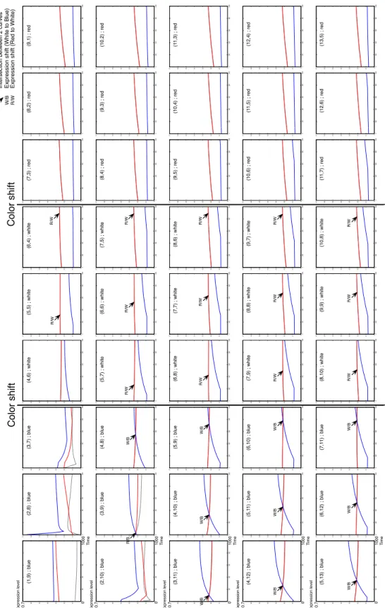
Bl ue W hi te R ed 0 0.1 0.2 0.3 0.4 0.5 0.6 0.7 0 200 400 600 800 1000 0 0.1 0.2 0.3 0.4 0.5 0.6 0.7 0 200 400 600 800 1000 0 0.1 0.2 0.3 0.4 0.5 0.6 0.7 0 200 400 600 800 1000 0 0.1 0.2 0.3 0.4 0.5 0.6 0.7 0 200 400 600 800 1000 0 0.1 0.2 0.3 0.4 0.5 0.6 0.7 0 200 400 600 800 1000 0 0.1 0.2 0.3 0.4 0.5 0.6 0.7 0 200 400 600 800 1000 0 0.1 0.2 0.3 0.4 0.5 0.6 0.7 0 200 400 600 800 1000 0 0.1 0.2 0.3 0.4 0.5 0.6 0.7 0 200 400 600 800 1000 0 0.1 0.2 0.3 0.4 0.5 0.6 0.7 0 200 400 600 800 1000 0 0.1 0.2 0.3 0.4 0.5 0.6 0.7 0 200 400 600 800 1000 0 0.1 0.2 0.3 0.4 0.5 0.6 0.7 0 200 400 600 800 1000 0 0.1 0.2 0.3 0.4 0.5 0.6 0.7 0 200 400 600 800 1000 0 0.1 0.2 0.3 0.4 0.5 0.6 0.7 0 200 400 600 800 1000 0 0.1 0.2 0.3 0.4 0.5 0.6 0.7 0 200 400 600 800 1000 0 0.1 0.2 0.3 0.4 0.5 0.6 0.7 0 200 400 600 800 1000 0 0.1 0.2 0.3 0.4 0.5 0.6 0.7 0 200 400 600 800 1000 0 0.1 0.2 0.3 0.4 0.5 0.6 0.7 0 200 400 600 800 1000 0 0.1 0.2 0.3 0.4 0.5 0.6 0.7 0 200 400 600 800 1000 0 0.1 0.2 0.3 0.4 0.5 0.6 0.7 0 200 400 600 800 1000 0 0.1 0.2 0.3 0.4 0.5 0.6 0.7 0 200 400 600 800 1000 0 0.1 0.2 0.3 0.4 0.5 0.6 0.7 0 200 400 600 800 1000 0 0.1 0.2 0.3 0.4 0.5 0.6 0.7 0 200 400 600 800 1000 0 0.1 0.2 0.3 0.4 0.5 0.6 0.7 0 200 400 600 800 1000 0 0.1 0.2 0.3 0.4 0.5 0.6 0.7 0 200 400 600 800 1000 0 0.1 0.2 0.3 0.4 0.5 0.6 0.7 0 200 400 600 800 1000 0 0.1 0.2 0.3 0.4 0.5 0.6 0.7 0 200 400 600 800 1000 0 0.1 0.2 0.3 0.4 0.5 0.6 0.7 0 200 400 600 800 1000 0 0.1 0.2 0.3 0.4 0.5 0.6 0.7 0 200 400 600 800 1000 0 0.1 0.2 0.3 0.4 0.5 0.6 0.7 0 200 400 600 800 1000 0 0.1 0.2 0.3 0.4 0.5 0.6 0.7 0 200 400 600 800 1000 0 0.1 0.2 0.3 0.4 0.5 0.6 0.7 0 200 400 600 800 1000 0 0.1 0.2 0.3 0.4 0.5 0.6 0.7 0 200 400 600 800 1000 0 0.1 0.2 0.3 0.4 0.5 0.6 0.7 0 200 400 600 800 1000 0 0.1 0.2 0.3 0.4 0.5 0.6 0.7 0 200 400 600 800 1000 0 0.1 0.2 0.3 0.4 0.5 0.6 0.7 0 200 400 600 800 1000 0 0.1 0.2 0.3 0.4 0.5 0.6 0.7 0 200 400 600 800 1000 0 0.1 0.2 0.3 0.4 0.5 0.6 0.7 0 200 400 600 800 1000 0 0.1 0.2 0.3 0.4 0.5 0.6 0.7 0 200 400 600 800 1000 0 0.1 0.2 0.3 0.4 0.5 0.6 0.7 0 200 400 600 800 1000 0 0.1 0.2 0.3 0.4 0.5 0.6 0.7 0 200 400 600 800 1000 0 0.1 0.2 0.3 0.4 0.5 0.6 0.7 0 200 400 600 800 1000 0 0.1 0.2 0.3 0.4 0.5 0.6 0.7 0 200 400 600 800 1000 0 0.1 0.2 0.3 0.4 0.5 0.6 0.7 0 200 400 600 800 1000 0 0.1 0.2 0.3 0.4 0.5 0.6 0.7 0 200 400 600 800 1000 0 0.1 0.2 0.3 0.4 0.5 0.6 0.7 0 200 400 600 800 1000 R/B W/B R/W W/B W/B W/B R/W W/B W/B W/B R/W W/B W/B W/B R/W R/W R/W R/W R/W R/W R/W R/W R/W R/W R/W 0 1000 0.7 0 1000 0.7 0 1000 0.7 0 1000 0.7 0 1000 0.7 Exp re ssi o n l e ve l Exp re ssi o n l e ve l Exp re ssi o n l e ve l Exp re ssi o n l e ve l Exp re ssi o n l e ve l T ime T ime T ime T ime T ime C o lo r sh if t C o lo r sh if t In te rse ct io n b e tw e e n 2 cu rve s W/B Exp re ssi o n sh ift (W h ite t o Bl u e ) R/W Exp re ssi o n sh ift (R e d t o W h ite ) (1 ,9 ) ; b lu e (2 ,8 ) ; b lu e (3 ,7 ) ; b lu e (2 ,1 0 ) ; b lu e (3 ,9 ) ; b lu e (4 ,8 ) ; b lu e (3 ,1 1 ) ; b lu e (4 ,1 0 ) ; b lu e (5 ,9 ) ; b lu e (4 ,1 2 ) ; b lu e (5 ,1 1 ) ; b lu e (6 ,1 0 ) ; b lu e (5 ,1 3 ) ; b lu e (6 ,1 2 ) ; b lu e (7 ,1 1 ) ; b lu e (4 ,6 ) ; w h ite (5 ,5 ) ; w h it e (6 ,4 ) ; w h it e (5 ,7 ) ; w h ite (6 ,6 ) ; w h it e (7 ,5 ) ; w h it e (6 ,8 ) ; w h ite (7 ,7 ) ; w h it e (8 ,6 ) ; w h it e (7 ,9 ) ; w h ite (8 ,8 ) ; w h it e (9 ,7 ) ; w h it e (8 ,1 0 ) ; w h it e (9 ,9 ) ; w h it e (1 0 ,8 ) ; w h it e (7 ,3 ) ; re d (8 ,2 ) ; re d (9 ,1 ) ; re d (8 ,4 ) ; re d (9 ,3 ) ; re d (1 0 ,2 ) ; re d (9 ,5 ) ; re d (1 0 ,4 ) ; re d (1 1 ,3 ) ; re d (1 0 ,6 ) ; re d (1 1 ,5 ) ; re d (1 2 ,4 ) ; re d (1 1 ,7 ) ; re d (1 2 ,6 ) ; re d (1 3 ,5 ) ; re d
Figure 4: Variation of the gene expression levels over time for each cell of the organism. The curves correspond to the regulatory network activity of each cell of the French flag. The coordinate and the color of the cell are given by the title of each curve. We can observe a strong link between the delay of expression of appropriate gene and the distance to the color shift: the longer the distance to the color shift point, the faster the gene expression.
Figure 3: Development of the French flag
the target flag. To study the spatialization of the regulatory network, we extract all the curves of the color expression level over time of the regulatory network expressed in each 45 cell of the organism. These curves are presented in figure 4. The top left curve matches with the left corner blue cell of the organism in figure 3.
All these curves represent the variation of the three gene expression levels (blue, white and red) on the y-axis (scaled between 0 and 1) during the one thousand time steps of reg-ulatory network’s evolution. In the top left part of the figure, both morphogen orientations are represented according to the organism orientation.
It is interesting to notice the progressive softening of the blue curve in all curves and, at the opposite, the progressive increasing of the two other curves (red and white are almost overlapped). On the one hand, the transition between the blue curve and the white/red curves is very visible. On the other hand, the transition between white and red is hugely more smoothy. Both curves are very close all the time, ex-cept in the 5 top left curves. This exex-ception is certainly due to a strong regulation shift in the regulatory network.
More relevant, the temporality of the color expression shifts is very observable. Considering only the blue and the white strips, the expression of the blue color is visible later and later in the regulatory network as the cell is closer to the white area.
The blue/white shift disappears from the curve when the cell must be white but we can assume by interpolation of the curves that the shift happens later. The same phenomenon is also present between the white and the red strips, as pointed out by the R/W black arrows. It exhibits the strong link be-tween the temporality of the gene expression and the
spatial-ity of the problem provided by the morphogen gradients. Figure 5 presents the extraction of the regulatory network
of the best evolved candidate. The nodes represent two
groups of genes: the regulation genes named G1 to G39 and the product genes (that will produce the color of the cell) named P1 to P99. The size of each node is proportional to its number of links. The architecture of this network is inter-esting to observe. First, almost all the genes are used. Only two genes (G23 and G33) are not linked to the regulatory network. It shows the total use of the genome and the com-plexity of the network extracted. Secondly, six genes (G5, G14, G16, G27, G28 and G38) are interfacing the regulatory network and all product genes except P2, which is directly linked to the regulatory network. The interface has not been coded in the network. It only emerged thanks to the evolu-tionary process. Lastly, in the regulatory area, three genes (G4, G25 and G26) play a central role and they are strongly connected to the rest of the regulatory area. This regula-tory area is very complex with a lot of links between all the nodes. This complexity is due to the necessity to exploit both gradients (horizontal and vertical).
The Japanese flag In order to investigate the
indepen-dence of the coordinate system to the temporality answer of the regulatory network, development of a japanese flag in a radial coordinate system is studied. The goal is thus to de-velop into an image with a red circle in the center of a white 13x9 rectangular shape (a total of 213 cells). The same three genes have been kept in order to establish the capacity of the GRN to switch off a particular gene.
G23 G33 Products Unused genes Regulatory area Interface genes Interface genes
Figure 5: Gene regulatory network extracted from the best genome of the French flag with a threshold value of 19. G-genes represent regulation G-genes and P-G-genes represent the products of the regulatory network (a color expression).
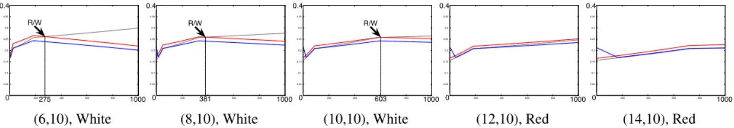
0 0.05 0.1 0.15 0.2 0.25 0.3 0.35 0.4 0 200 400 600 800 1000 R/W 275 0.4 0 1000 0 0.05 0.1 0.15 0.2 0.25 0.3 0.35 0.4 0 200 400 600 800 1000 R/W 0.4 0 381 1000 0 0.05 0.1 0.15 0.2 0.25 0.3 0.35 0.4 0 200 400 600 800 1000 R/W 0.4 0 603 1000 0 0.05 0.1 0.15 0.2 0.25 0.3 0.35 0.4 0 200 400 600 800 1000 0.4 0 1000 0 0.05 0.1 0.15 0.2 0.25 0.3 0.35 0.4 0 200 400 600 800 1000 0.4 0 1000
(6,10), White (8,10), White (10,10), White (12,10), Red (14,10), Red
Figure 6: Gene expression level curves of 5 cells of the Japanese flag’s central line. The curves’ legends indicate the coordinate and the color of the cell that correspond to the gene expression.
As previously, only 15 generations is required to obtain a near-perfect flag (with only 3 pixels wrong). Figure 7 illus-trates the flag obtained.
As for the previously presented French flag, all the curves of the gene regulation have been extracted in order to study the link between the temporality of the regulation and the spacialization of the problem. Figure 6 shows the curves of gene expression levels of five cells of central line: 3 whites cells and 2 red.
We can observe that all the expression levels are very close (y-axis is zoomed on the interval [0, 0.4]). The blue gene is also very strongly expressed even if not needed in this flag. Its inhibition by the regulatory network is correctly made but seems to be very weak. The same link between the temporality and the distance to the shift is also observable as on the French flag: the closer the colors shift, the later the gene expression levels shift. The same behavior is observ-able elsewhere on the flag and each transition stage can be obtained by rotation.
Conclusions and Perspectives
The goal of this work was to investigate the use of Artifi-cial GRN in the context of a spatial problem. We combined Banzhaf’s GRN model to our own developmental model Cell2Organ, and experimental studies have been conducted on variations of the multi-cellular flag problem, a well-known benchmark in Artificial Embryogeny. Results from
Figure 7: Development of a Japanese flag with a radial gra-dient.
the experiments confirm the strong link between the tempo-rality of the gene expressions in the regulatory network and spatial parameters of the problem. Indeed, change in the cell differentiation process among the organism is correlated by significant shifting in the GRN dynamics. The temporal as-pect observed here also raises numerous question regarding the ability of a population of GRN to actually generate some desired behaviors. How many steps does it take to produce a correct output? What is the expressivity of such a system, in particular, how many basin of attractions can be encoded within one GRN template? Is it possible to have, depending on the context at hand, either a fast or a smooth shift between two regimes? These questions are of particular interest to explore further GRN-based control optimization problems (Joachimczak and Wr´obel, 2010; Nicolau et al., 2010).
The complexity of the regulatory network obtained was also somewhat surprising and raises the question as to the evolvability of such a representation. The regulatory net-work needed a large number of P-genes (not restrained in these experiments) in order to find a solution to the prob-lem. This may be a symptom of code bloat, a well-known problem of uncontrolled growth in variable length represen-tations and definitely requires further studies, with possible investigations with respect to penalizing bloat without un-dermining the model’s performance.
Lastly, spatial problems addressed here are relevant for this kind of detailed study, but have limited applications in the current form. However, the field of applications is large and examples from Biology give a good indications on the variety of problems to be addressed: cell differentiation into neurones, development of muscular cell, tissues, etc. In the context of computer modelling, understanding the intrinsic properties of GRN may be relevant in a variety of prob-lems requiring complex temporal and spatial interactions. Indeed, because of their structure, regulatory networks could be more suitable for continuous problems than other behav-ior controlers such as artificial neural networks or classifier systems.
Acknowledgements
The authors would like to thank Miguel Nicolau for his help regarding the implementation of the artificial GRN model.
References
Banzhaf, W. (2003). Artificial regulatory networks and ge-netic programming. Gege-netic Programming Theory and Practice, pages 43–62.
Bowers, C. (2005). Simulating evolution with a compu-tational model of embryogeny: Obtaining robustness from evolved individuals. Lecture notes in computer science, 3630:149.
Chavoya, A. and Duthen, Y. (2008). A cell pattern gener-ation model based on an extended artificial regulatory network. Biosystems, 94(1-2):95–101.
Cussat-Blanc, S. Pascalie, J., Luga, H., and Duthen, Y. (2010a). Morphogen positioning by the means of a hy-drodynamic engine. In Artificial Life XII, pages 118– 125. MIT Press, Cambridge, MA.
Cussat-Blanc, S., Luga, H., and Duthen, Y. (2008). From single cell to simple creature morphology and metabolism. In Artificial Life XI, pages 134–141. MIT Press, Cambridge, MA.
Cussat-Blanc, S., Pascalie, J., Luga, H., and Duthen, Y. (2010b). Three simulators for growing artificial crea-tures. In Proceedings of the IEEE Congress on Evolu-tionary Computation (IEEE CEC 2010).
Davidson, E. H. (2006). The regulatory genome: gene reg-ulatory networks in development and evolution. Aca-demic Press.
Devert, A. (2009). Building processes optimization: Toward an artificial ontologeny based approach. PhD thesis, Universit´e Paris-Sud 11.
Doursat, R. (2008). Organically grown architectures: Creat-ing decentralized, autonomous systems by embryomor-phic engineering. Organic Computing, pages 167–200. Eggenberger, P. (1997). Evolving morphologies of simu-lated 3d organisms based on differential gene expres-sion. In Proceedings of the Fourth European Confer-ence on Artificial Life, pages 205–213. MIT Press Cam-bridge, MA.
Jaeger, H. (2001). The echo state approach to analysing and training recurrent neural networks. submitted for pub-lication.
Jakobi, N. (1995). Harnessing morphogenesis. In Interna-tional Conference on Information Processing in Cells and Tissues.
Joachimczak, M. and Wr´obel, B. (2008). Evo-devo in sil-ico: a model of a gene network regulating multicellular
development in 3d space with artificial physics. In Pro-ceedings of the 11th International Conference on Arti-ficial Life, pages 297–304. MIT Press.
Joachimczak, M. and Wr´obel, B. (2010). Evolving Gene Regulatory Networks for Real Time Control of Forag-ing Behaviours. In ProceedForag-ings of the 12th Interna-tional Conference on Artificial Life.
Knabe, J., Schilstra, M., and Nehaniv, C. (2008). Evolution and morphogenesis of differentiated multicellular or-ganisms: autonomously generated diffusion gradients for positional information. Artificial Life XI, 11:321. Lindenmayer, A. (1971). Developmental systems without
cellular interactions, their languages and grammars. Journal of Theoretical Biology, 30(3):455.
Miller, J. (2003). Evolving Developmental Programs for Adaptation, Morphogenesis, and Self-Repair. In Ad-vances in Artificial Life, pages 256–265. Springer. Mjolsness, E., Sharp, D., and Reinitz, J. (1991). A
connec-tionist model of development. Journal of theoretical Biology, 152(4):429–453.
Nicolau, M., Schoenauer, M., and Banzhaf, W. (2010). Evolving genes to balance a pole. Genetic Program-ming, pages 196–207.
Rechenberg, I. (1994). Evolution strategy. Computational Intelligence: Imitating Life, pages 147–159.
Reil, T. (1999). Dynamics of gene expression in an artifi-cial genome - implications for biological and artifiartifi-cial ontogeny. Advances in Artificial Life, pages 457–466. Schramm, L., Valente Martins, V., Jin, Y., and Sendhoff, B.
(2010). Analysis of Gene Regulatory Network Motifs in Evolutionary Development of Multicellular Organ-isms. In Proceedings of the 12th International Confer-ence on Artificial Life.
Stanley, K. (2004). Efficient evolution of neural networks through complexification. PhD thesis, The University of Texas at Austin.
Thomas, R., Thieffry, D., and Kaufman, M. (1995). Dynamical behaviour of biological regulatory net-worksi. biological role of feedback loops and prac-tical use of the concept of the loop-characteristic state. Bulletin of Mathematical Biology, 57:247–276. 10.1007/BF02460618.
Wolpert, L. (1968). The french flag problem: A contribu-tion to the discussion on pattern development and reg-ulation. Towards a theoretical biology, 1:125–133.