HAL Id: hal-02987268
https://hal.archives-ouvertes.fr/hal-02987268
Preprint submitted on 3 Nov 2020
HAL is a multi-disciplinary open access archive for the deposit and dissemination of sci-entific research documents, whether they are pub-lished or not. The documents may come from teaching and research institutions in France or abroad, or from public or private research centers.
L’archive ouverte pluridisciplinaire HAL, est destinée au dépôt et à la diffusion de documents scientifiques de niveau recherche, publiés ou non, émanant des établissements d’enseignement et de recherche français ou étrangers, des laboratoires publics ou privés.
Corruption, Tax reform and Fiscal space in Emerging
and Developing Economies
Djedje Hermann Yohou
To cite this version:
Djedje Hermann Yohou. Corruption, Tax reform and Fiscal space in Emerging and Developing Economies. 2020. �hal-02987268�
fondation pour les études et recherches sur le développement international
LA FERDI EST UNE FOND
ATION REC ONNUE D ’UTILITÉ PUBLIQUE . ELLE ME T EN ŒUVRE A VEC L ’IDDRI L ’INITIA TIVE POUR LE DÉ VEL OPPEMENT E
T LA GOUVERNANCE MONDIALE (IDGM).
ELLE C
OORDONNE LE LABEX IDGM+ QUI L
’ASSOCIE A U CERDI E T À L ’IDDRI. CE TTE PUBLIC
ATION A BÉNÉFICIÉ DU SOUTIEN DU MINIST
ÈRE DE L ’EUR OPE E T DES AFF AIRES É TR ANGÈRES .
Abstract
Several studies have demonstrated that corruption hinders efforts in enhancing
public revenue and fiscal space through different channels. This paper assesses the
effect of tax reform on fiscal space conditional on corruption control for a large panel
of developing and emerging economies over 1990-2016. Using a threshold approach,
our findings indicate that tax reform effect on fiscal space is not monotonic and
depends on corruption control. Tax reform enhances fiscal space and tax revenue
when corruption control is better. The results also suggest that heterogeneity across
countries and time does matter. Individual estimates of elasticity of fiscal space to
tax reform support evidence that countries that benefit most from tax reform are
those that prove enough ability to control corruption.
Keywords: Corruption, tax reform, Fiscal space, threshold, developing countries. Acknowledgments
I am grateful to Jose Gijon, Thierry Yogo respectively from the International Monetary Fund and the World Bank, and N’dri Marie-Christelle from London School of Economics in England, Michael Goujon and Patrick Guillaumont from the Foundation for Studies and Research on International Development in Clermont-Ferrand (France) for their helpful comments. The views expressed in this document are those of the author and do not necessarily represent those of the International Monetary or its policy.
Hermann D. Yohou, International Monetary Fund, Abidjan
contact : hyohou@imf.org
Corruption, Tax reform and
Fiscal space in Emerging and
Developing Economies
Hermann D. Yohou
Poli tiques de développem en t Docu ment de travail July 2020269
“Sur quoi la fondera-t-il l’économie du monde qu’il veut
gouverner? Sera-ce sur le caprice de chaque particulier? Quelle
confusion! Sera-ce sur la justice? Il l’ignore.”
Introduction
Adequate domestic revenue mobilization is essential to creating fiscal space and supporting sustainable growth as it strengthens the government’s ability to invest in growth-enhancing sectors without generating debt or jeopardizing economic growth. This critical role played by domestic revenue mobilization has been emphasized, inter alia, in the policy frame of the implementation of the millennium development goals and reiterated in that of the new Sustainable Development Goals (SDGs). To fulfill this crucial role, the mobilization of domestic revenue must be supported by a well-designed reform that could ensure a steady and stable increase in government revenue. But this could be hampered by poor governance, in particular corruption. Over the past two decades, the reforms put in place to boost domestic revenue mobilization in developing countries have
mainly consisted of policies that enhance tax revenue collection by strengthening the capacity of
tax administration and promoting a better composition of tax revenue. At the same time, governments have strived to improve governance and institutional frameworks, amongst others, by strengthening their citizens’ participation in policymaking and establishing audit and anti-corruption institutions that maximize the tax reforms’ outcome. However, despite these efforts, many developing countries have not generated much fiscal space to address their development needs because of insufficient domestic revenue. For instance, government revenue in Low-Income Developing Countries (LIDCs) has steadily decreased from 16.9 on average in 2010 to 15.3 as percent of GDP in 2019 whereas the number of them facing serious debt challenges has more than doubled from 21 in 2013 to 43 countries in 2019 as a result of increased fiscal deficits from -2.8 in 2010 to -4.2 as percent of GDP in 2019; despite a strong positive economic growth around 5 percent on average (International Monetary Funds (henceforth IMF), 2019a,b,c). These mixed performances achieved so far have raised questions about the quality of the implementation of the reforms and the role of persistent factors that continue to limit their effectiveness.
Some studies have been devoted to examining the role of institutional factors in fiscal space expansion and highlight that they play a crucial role in enhancing government revenue (Yohou et al., 2016; Bird et al, 2008). Among these institutional variables, corruption is undoubtedly considered as the variable with the most potential harmful effects on public finances (Shleifer and Vishny, 1993; Mauro, 1995; Ades and Di Tella, 1997; Rose-Ackerman and Coolidge, 1997; Wei, 1997; World Bank, 1997; Mauro, 1998; Hindriks et al., 1999, Attila et al. 2009). A recent International Monetary Fund’s report notes that for countries with similar level of income, the least corrupt countries collect about
4 percent tax to GDP higher than the most corrupt countries (IMF, 2019a). Ghura (1998) finds that increased corruption lowers tax revenue in Sub-Saharan African countries.
Whilst most studies focus on the correlation between corruption and government revenue, this paper investigates the pass-through effect of corruption on fiscal space via tax reforms. Tax reforms are essential to broadening tax base, increasing government revenue efficiency, and supporting development goals which, in turn, will strengthen the fiscal space expansion. But corruption can hinder these beneficial effects on fiscal space through multiple channels. First, it can prevent the necessary tax reforms or thwart their implementation. When decisions are guided by bribes and nepotism, governments are unable to make effective tax reforms, which reduce the positive impact of the implemented reforms and consequently leads to lower fiscal outcomes. Second, corruption can reduce fiscal space by undermining the quality of public spending, hence deteriorating citizens’ trust in government, and eroding any advances in policies which support tax compliance. Moreover,
corrupt governments are more subject to the pressure of lobbies benefitting of exemptions 1 or
loopholes who are more inclined to prevent tax reform aiming at greater equity and broadening tax base. Higher inequality and narrow tax base will translate in lower revenue and fiscal space. Corruption can skew tax collection towards taxes that are easy to collect such as customs tariffs but
very subject to bribes (Attila et al., 2009; Imam and Jacobs, 2014; Liu and Mikesell, 2019). By
weakening tax reform, corruption lessens the level of government revenues. Lower revenues induce borrowing which augments its servicing (Cooray et al, 2017), which in turn reduces fiscal space. Furthermore, as broadly evidenced in the literature (Mauro, 1995, 1998; Tanzi and Davoodi, 1997; 2000), corruption can weaken tax base and leads to lower tax revenues and fiscal space by deterring economic growth. Finally, strong institutions are particularly necessary for the proper design and success not only of reforms in the fiscal area, but also of all the reforms in other areas— such as financial inclusion reforms, education— which indirectly contribute to the effectiveness of fiscal
reforms. But in a corrupt environment, such institutions are unlikely to exist as corruption is a
self-perpetuating scourge that can divert reforms resource and impairs their quality.
However, despite broad evidence of adverse effects, some authors claim that corruption might enhance efficiency and growth under circumstances such as friendly-distortive policies, chronic administrative backlog. Akdede (2011), for instance, finds support that sufficiently large bribe from government officials incites citizens to pay taxes voluntarily, instead of evading payment. Alm et al.
(2016) also find that whilst corruption increases tax evasion, excessive corruption can induce an
atmosphere that is conducive to compliance. These studies then suggest that the effects of corruption on fiscal space are potentially nonlinear.
This paper aims to examine the effect of tax reforms on fiscal space conditional on the level of corruption for a panel of 64 developing and emerging countries over the period 1990-2016. We argue that corruption deteriorates the potential positive effects of tax reforms on fiscal space. We specifically highlight the heterogeneous effect of tax reforms assuming that it gradually changes over time and across countries as the level of corruption varies in respect with an endogenously determined threshold. We econometrically approach this assumption by relying on the Panel Smooth Threshold Regression model as developed by González et al. (2005), Fok et al. (2005). Tax reform is measured by a composite index of the similarity of non-resource tax revenue composition to advanced countries to keep in line with the fact that recent tax reforms in developing countries have focused on shifting their tax revenue structure towards that of advanced economies (Gnangnon and Brun, 2019; Gnangnon, 2019; and Yohou, 2019).
Considering the debt service to tax ratio as our main fiscal space variable of concern, we find that though tax reform does not robustly affect fiscal space, its effect statistically increases gradually across countries as corruption control index increases. Likewise, the results show that tax revenue is associated with higher tax reform and that corruption control statistically enhances this relationship. Furthermore, regardless of the region or the income groups to which they belong, the magnitude of the effects varies from one country to another depending on the level of corruption that prevails, so that for countries with similar income, tax reform may have less impact on fiscal space for a country with high corruption.
The remainder of the paper is organized as follows. Section 2 presents some stylized facts about corruption, fiscal reforms and performances in terms of fiscal space in developing countries. Section 3 presents the data and the estimation method. Section 4 concerns the interpretation of the estimates while Section 5 draws the implications and concludes.
2. Corruption, quality of public policies and fiscal space in developing and emerging countries
Fiscal space is defined as a government's ability to finance its priority expenditures without compromising its solvency and that of the economy. This implies that the government can raise expenditure or modulate taxes without jeopardizing the debt sustainability and compromising market access. Corruption can affect fiscal space by affecting its key components and the factors that support them. This section revisits control of corruption and fiscal performances along with their relationships with key policy variables that lead to the expansion of fiscal space.
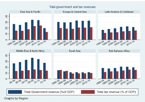
Figure 1 depicts the level of revenue mobilization—total government revenues and total tax revenues as percent of GDP— for 64 developing and emerging countries across regions over 1990-2016. First, it shows some heterogeneities across regions and that revenue collection is lower in South Asia and Sub-Saharan Africa than the rest of the developing world. Government revenue to GDP is on average 12.3 and 19.4 percent in South Asian and Sub-Saharan African regions respectively. It is 20.2 percent in LAC against 29.2 percent in East Asia and Pacific. European and Central Asian and MENA developing countries record the largest share of revenue with respectively 31.5 and 31.4 percent. Government revenues’ performances are mainly owed to tax collection, both total and tax revenues variables being positively associated. Tax revenues represent about 70 percent of total government revenues. Tax to GDP ratio is 13.7 percent on average in SSA and 10.6 percent in SA against 20 and 18.8 percent in Europe and central Asia developing countries and Eastern Asian and Pacific region. While the graph shows some heterogeneities across regions, both government revenue and taxes have increased slightly except South Asia that shows a steady downward trend since 1990s and to some extent EAP and MENA. Revenue collection improved in EAP from 26.8 percent over the period 1990-1994 to 29.2 percent over the period 2010-2014 before declining to 19.6 percent in 2015-2016. MENA exhibits similar trend while SSA improved only slightly from 18.8 percent over 1990-1994 to 19.1 percent over 2014-2016 in contrast with tax revenue that increased by 2.9 points of GDP over the same period.
Figure 1: Total government and tax revenues as percent of GDP
Source: Authors from International monetary Fund
The PRSP Group releases yearly data on corruption index—The ICRG corruption index— which measures the actual and potential risk of corruption within the political system that reduces the efficiency of government and business by enabling people to assume positions of power through patronage rather than ability. These include demands for special payments and bribes connected with government operations including tax assessments, excessive patronage, nepotism, job reservations, ‘favor-for- favors’, secret party funding, and suspiciously close ties between politics and business (The PRSP Group, 2018). Because, the higher the index, the lower the risk of corruption, the lower index the higher the risk of corruption, we prefer to use the terms of corruption control. Figure 2 shows the status of the index across regions and in selected countries over the period 1990-2016. It highlights a significant decline in control of corruption across the regions over time suggesting that corruption has increased in developing countries. Control of corruption index decreased from 4 in 1990 to 2.3 in 2016, suggesting that perception that corruption has almost doubled in two decades. This evolution demonstrates that there is scope to materialize the effects of commitments to reducing corruption in developing and emerging economies. By contrast, corruption control in South Asia improved significantly from 1.5 to 2.8 in 2016 although it recorded a slight deterioration between 2000 and 2010. Since 2000, the SSA has experienced the weakest level of corruption control.
Although there is not much variation across the regions on average over the last two decades, individual heterogeneities do exist over time. The second graph on figure 2 plots the evolution of control of corruption index in selected countries to highlight these heterogeneities. They include Angola, Albania, Cote d’Ivoire and Cameroon. It shows that corruption control evolves differently for countries with similar level of development even if the general downward pattern is noticed over the entire period. The evolution is erratic across countries. Corruption control index in Albania has unsteadily passed from 4 in 1990 to 1 in 2006 before being on an increasing path tough the latter is nonlinear. The graph of Cote d’Ivoire takes an alternative inverted U and U shapes before an upward trend since 2012. Despite the echo of being among top reformer countries since 2012 and improvement in rankings, the Ivorian performances are insufficient to reach its historical pick of 4 in 1995, the same applies to Albania. But the downward trend of Angola has remained continuous since 1990 passing from 3 to around 1 whereas that of Cameroon is getting stabilized around 2 after an inverted U shape from 2005 (3.7) to 2012.
Figure 2: Compared corruption control in developing and emerging countries, 1990-2016Source:
Authors from ICRG database
These different patterns of corruption control may result in heterogenous corruption’s effects on outcome over time and across countries. The predominance of the current status of corruption in developing and emerging countries despite echoed commitments towards its reduction is of concern. It could highlight the still lagging positive effects of the numerous institutional and revenue mobilization reforms to tackle the inadequate financing that retards their development.
Corruption can hamper fiscal space through its direct unfavorable effect on government revenue and tax collection. Theoretical and empirical evidences suggest that corruption lowers revenue collection because of tax fraud, tax evasion, and diversion of the collected taxes towards the tax collectors own’s use, weaker tax structure. Focusing on a panel of 39 African countries over 1985-1996, Ghura (1998) demonstrates that tax revenues decline with corruption. Tanzi and Davoodi (2000) point out that corruption hampers total tax revenues and that this effect differs according to the category of the tax considered in cross-section analyses. Thornton (2008), Attila et al. (2009), Imam and Jacobs, (2014), Baum et al. (2017) also evidence similar findings that not only corruption has a negative effect on public revenues collection, but also modulates tax structure in favor of the tariffs while dipping direct and indirect revenues owing to rent-seeking. Uslaner (2010) presents empirical findings that cover 27-28 transition economies from 2002 to 2005, which suggest that corruption negatively impacts tax payment decision. Along the same line, Alm et al. (2016) demonstrate both theoretically and empirically that corruption largely contributes to firms’ tax evasion.
Figure 3 below plots the relationship between corruption control index and fiscal performances including the level of tax, debt and the efficiency of revenue collection from the World Bank's Country Policy and Institutional Assessment (CPIA). It highlights a positive correlation between corruption control and efficiency in revenue mobilization and fiscal performances. Countries with higher corruption control tend to have higher total government and tax revenues to GDP ratios. In contrast, better corruption control is associated with lower stock of public debt. The quality of institutions plays an important role in determining a country’s level of development as well as its fiscal space. However, corruption can erode these important fundamentals. It is well demonstrated in the literature that institutions are essential elements for development (Acemoglu and Robinson, 1999; Acemoglu et al., 2005) and revenue mobilization to take place (Bird et al., 2008, 2014; Yohou et al., 2016, etc.). Despite widespread evidence in the literature that the pervasive effects of corruption are reduced when institutions are good, corruption itself is subject to increasing returns which perpetuate it (Tanzi and Davoodi, 2000) by debasing other aspects of institutions, among them that of accountability, stability, auditing, even leading to their collapse.
Figure 3: Control corruption and fiscal performances
Source: Authors from ICRG, IMF.
This induced decline in the quality of institutions will transmit to development through lower growth, the diversion of talents and inappropriate dedication to address the issue of poverty. A Lower level of development leads to inadequate economic composition skewed towards sectors that contribute less to taxes such as agriculture, and less financial development, which limits government’s capacity. All the above factors will eventually erode a country’s tax base. A reduced tax base due to lower development, in turn, has unfavorable effects on the efficiency of a country’s fiscal system, as it translates into tax harassment of an already sparse population of taxpayers, encouraging tax evasion. This will result in inadequate public resources vis-à-vis the needs of the
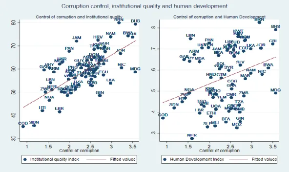
society. Figure 4 depicts a positive association between corruption control and institutional quality2
on one hand, and between corruption control and human development index on the other. Countries that are lagging in corruption control such as Democratic Republic of Congo, Nigeria, Zimbabwe, and Haiti are those lagging in institution quality and in human development.
2
The institutional quality index is the composite political risk index from the ICRG database, which is the sum of all the 12 major
components in this category ranging from 0 to 100 points. This index contains: government stability, socioeconomic conditions, investment profile, internal conflict and external conflict, rated from 0 to 12, with corruption, military in politics, religious tensions, law and order, ethnic tensions, and democratic accountability, rated from 0 to 6, and bureaucracy quality, rated from 0 to 4. The higher the value of the component, the lower the associated risk perceived (Yohou et al., 2016).
Figure 4: Corruption control, institutional quality and human development
Source: ICRG database and United Nations Development Program (UNDP).
As aforementioned, the environment surrounding the definition and implementation of the required policies does matter for their quality and effectiveness. As argued by Tanzi and Davoodi (1997) in a case of public investment projects, corruption can distort the decision-making process and result in lower productivity. A corrupt environment facilitates the consolidation and control over reforms by corrupt elites looking to securing their advantages, which, in turn, results in lower social inclusion and poor quality of fiscal management. Accordingly, the incentive to avoid tax payment will go hand in hand with bad reforms and will lead to an inefficient and weak fiscal system which will contribute to deteriorating the tax moral and social bargaining. A recent fiscal monitoring by the IMF on the effect of corruption stresses that corruption impairs the effectiveness of government policies through the distortion of incentives of policymakers and civil servants and weakened core public services such as the provision of good infrastructure and education. Hanousha and Palda (2004) present similar conclusion that the perceived quality of government services determines the willingness to pay or evade taxes. Uslaner (2010) argues that corruption decreases tax compliance by weakening the social contract between citizens and government, by promoting feeling of inequity and unfairness. He supports that tax compliance in transition economies reflect citizens’ perception of the quality of services and the level of corruption, both in the tax administrations and throughout the entire society including the government. Similar lessons can be drawn from several individual and co-authored papers of Torgler which highlight that tax moral is closely related to trust in government that corruption tends to undermine (Togler, 2003a,
b; Torgler et al., 2008; Bird et al., 2008; Bird et al., 2014). Figure 5 provides supports for the claim that corruption is harmful to the factors that promote tax compliance and effectiveness of the necessary fiscal reforms. In fact, the control corruption index exhibits a strong positive correlation with the CPIA transparency, accountability, quality of budgetary and management, equity of the use of public resources and social inclusion indicators.
Figure 5: Corruption control, quality of fiscal policies management and inclusion
Source: Authors from ICRG and World Bank
This section shows that corruption can hinder fiscal space through several factors including the quality of institutions and fiscal reforms. By all means, correlation does not necessarily mean causation. But considering the evidence in the literature, we can provide first insight into the
potential effects of corruption. Studying all the channels through which corruption affects fiscal
space is beyond the scope of the current study. We test for the significance of the channel of tax reform —whether or not tax reform is a significant channel of the impact of corruption on fiscal space— taking advantage of the potential implication of the cross-country heterogeneities in corruption.
3. Econometric model and data
Our aim is to examine the conditional effect of tax reform on fiscal space depending on corruption control in developing countries. We resort to the Panel smooth threshold regression (PSTR) model as developed by Fok et al. (2005) and González et al. (2005). The PSTR is an extension of the abrupt panel threshold model à la Hansen (1999). It allows to highlight the heterogeneous gradual and individual effects according to the level of control of corruption. Yohou et al. (2016 and 2016) have
used this approach to estimate the aid-tax relationship upon government stability.
3.1. Model specification
We use two dependent variables to check the robustness of the results. The main dependent
variable of interest is a de facto fiscal space that we measure by the ratio of public and publicly
guaranteed debt service to the total government revenue excluding grants. It measures the burden of public debt service in respect to government revenues. It provides a good indication of a country’s available budgetary room for financing its activities after servicing its debt. The higher the ratio, the lower the room and hence the lower the fiscal space. This ratio is one of the key indicators of the IMF and World Bank debt sustainability analysis to measure a country’s risk of indebtedness. The second dependent variable is total tax revenues as percent of GDP. Tax revenue is a key variable of fiscal space because it accounts for a substantial share of public revenue. It is widely used to compare countries’ revenue performances and to measure de facto a country’s effort to ameliorate its fiscal space (Pessino and Fenochietto, 2010; Bird et al., 2008; Brun et al., 2015; Garg et al., 2017; Yohou and Goujon, 2017).
The key variable of interest is the tax reform index from Yohou (2019) who built it based on the work of Gnangnon and Brun (2019) and Gnangnon (2019). It is a composite index of the structure of non-resource tax revenue and measures the degree by which developing countries’ tax structure
is similar to that of the “traditional” advanced economies3. It is built following the semi-metric
Bray-Curtis (1957) dissimilarity index:
3 Following Gnangnon and Brun (2019) and Gnangnon (2019), traditional advanced economies are the following
countries: Australia, Austria, Belgium, Canada Denmark, Finland, France, Germany, Greece, Japan, Luxembourg, Netherlands, New Zealand, Norway, Portugal, Spain, Sweden, Switzerland.
1 ( ) ( ) ( ) it t it t it t it it t it t
dirtax adedirtax indirtax adeindirtax tradtax adetradtax
Taxreform
dirtax adedirtax indirtax adeindirtax tradtax adetradtax .
Where dirtax ,it indirtax and it tradtax denote respectively the direct taxes, indirect taxes and trade it
taxes excluding resource revenue as percent of GDP for the developing economy iat period t. The
suffix “ade ” indicates the corresponding average tax component for advanced economies at period t
t. The higher the index, the higher the quality of the tax reform. Regarding the threshold variable,
we use the control of corruption index, CCorruption , from the International Country Risk Group (ICRG). It is bounded between 0 and 6. Higher values of the index indicate less corruption. The modeling of the fiscal space function as part of a panel smooth threshold effect is defined by the following equation:
' ' ' '
0 1 ( , , ) 2 it
it i c it it it it it
FiscSpace c Taxreform Taxreform g CCorruption CCorruption X u (0.1)
Where i 1,...,n represent countries and t1,...,T time periods. FiscSpace denotes the fiscal space
variable, the vector of control variables X reflects the quality of institutions, the macroeconomic it
performances, the trade openness, the demographic dimension, the level of development, and the
government expenditure size. '
, ,..2 j c
are the vectors to be estimated. i
and
u are the fixed itindividual effects and the errors, respectively. The errors are assumed to be i.i.d. As said above,
it
CCorruption is the index of control of corruption in countryiand periodt. The transition function
( it, , )
g CCorruption CCorruption is a continuous function of the threshold variable, so that the value
of CCorruption determines the value of it g CCorruption( it, , CCorruption). Hence, the effect of tax
reform on fiscal space for country iat period t is given by:
0 1 ( ; ; ) it it it FiscSpace g CCorruption Ccorruption Taxreform (0.2)
The value of the transition function ranges from 0 to 1 and defines the two extreme regimes. If it
equals 0, the effect of tax reform equals 0, and if it equals 1, the effect of tax reform equals 0 1
.
Following Granger and Teräsvirta (1993) and González et al. (2005), g takes the following logistic
function: 1 ; 1 ( it ; ) 1 exp( m ( it j) j
g Ccorruption Ccorruption Ccorruption Ccorruption
Where CCorruption Ccorruption Ccorruption( 1,...,Ccorruptionm)is a m-dimensional vector of location parameters and the estimated term is the slope of the transition function. A key advantage of the PSTR consists of allowing coefficients of tax reform to vary between countries and over period. It provides a parametric approach to modelling cross-country heterogeneity and the time instability of the tax reform coefficients, since these parameters vary as a function of the threshold variable, the control of corruption index. As a consequence, we are able to estimate many values of the tax
reform effect coefficients, lying between 0 and 0 , as country-period observations. However, 1
this results in the difficult task of trying to give sound interpretation to the size of the tax reform
effect estimates in equations (1.1). Thereupon, the signs of 0 and 1 are the only elements that
should be interpreted rather than their values. Concerning the slope parameters , it determines
the shape of the transition function. When it equals 0, the transition function translates into a constant and the model corresponds to the standard linear model with individual effects, i.e. coefficients are constant and homogeneous. By contrast, when it tends toward infinity, the transition function becomes an indicator function, the PSTR model translates into the two-regime
Panel Threshold Model à la Hansen (1999) if m 1 for instance. If m f 1 and tends to infinity, the
number of regimes remains 2 while the function switches between 0 and 1 (Colletaz et Hurlin, 2006; Yohou et al., 2016).
The quality of institutions is positively correlated to fiscal space (Aizenman et al., 2019) through its capacity to effect the efficiency of tax collection and encourage tax compliance, the end result being higher public revenues (Tanzi and Davoodi, 1997; Ghura, 1998; Torgler, 2003a, b; Torgler et al., 2008; Bird et al., 2008 and 2014; Yohou et al., 2016, Aizenman et al., 2019). Greater public revenues will, in turn, result in lower debt to finance the needed infrastructure or better financing conditions. We therefore expect a negative correlation between the quality of institutions and the fiscal space indicator but positive correlation with tax to GDP ratio. The quality of institutions is captured by a composite index using a principal component analysis on ICRG 12 indices and the full ICRG
database including all the surveyed countries to allow international comparison.4 Details could be
provided upon request.
Economic growth—measured by the variation in percentage of the GDP— is expected to be positively correlated with greater fiscal space, as stronger growth leads to higher government
revenues and lowers the reliance on debt, and consequently lowers debt service. The sign of the coefficient of economic growth variable is expected to be negative whilst that of tax revenue positive.
The effect of trade openness is ambiguous. There is evidence of contrasting effects on fiscal space (Agbeyegbe et al., 2006; Hines and Summers, 2009; Le et al. 2012; Gnangnon and Brun, 2019), its effects could be either positive or negative. Trade can trigger growth and raise public revenues and alleviate debt burden and its service. In contrast, greater trade openness can reduce borders taxes as a result of declining tariffs and reduced number of border duties which in turn hinder tax and fiscal revenues. Moreover, financial pressures on government spending from increased globalization is likely to induce costly tax collection and higher economic distortions (Hines and Summers, 2009). Amid these potential conflicting effects of trade on fiscal space and tax revenues, we assume that the positive effects will outweigh the adverse effects. Trade openness is measured by the ratio of sum of imports and exports to GDP.
Population growth captures the role of changes in demographics. A growing population may suggest that the labor force is increasing and could potentially be taxed leading to an increase in government revenues and fiscal space. However, in a context of weak tax system capacity, for those countries included in this study, it proves difficult to capture the fast-growing population as well as the limiting fiscal space. But faster population growth may also result in higher age dependency ratio and increase the demand for more public services such as education and health care that will demand more tax revenues. We expect the effect to be either positive or negative on fiscal space. The rate of Inflation is measured by the percentage change in consumer price. While the so-called Oliveira-Tanzi effect predicts a negative relationship between the rate of inflation and government revenues (as it affects the real value of taxes), the rate of inflation is potentially harmful to public debt service so that the effect could be mixed. Real GDP per capita is a proxy of level of income or development. An increase in real GDP translates into an increase in national wealth, higher revenue base and hence a greater financing capacity. Caeteris paribus, an increase in real GDP is conducive to an increase in fiscal space. In addition, according to Bird et al. (2014), higher level of development is associated with greater tax effort as it implies higher capacity of paying and collecting taxes as well as higher relative demand for income elastic public goods and services that would need to be taxed. These factors compound to have a positive relationship between higher level of development and tax revenue and larger fiscal space (a negative relationship with the fiscal space indicator).
Finally, following Cyan et al. (2013), we include the general government final consumption as percentage of GDP to capture the effects of government size on fiscal space. The authors demonstrate that tax effort measurement should be accounted for budgetary needs as the level of needed tax revenue in any country depends on the collective choice of the desired level of public expenditure. In line with them, we expect a positive effect of the government size on fiscal space efforts. Hence, we expect negative and positive signs of government expenditure with the fiscal space and tax revenue to GDP indicators, respectively.
3.2. Estimations and tests of the specification
Following Gonzales et al. (2005) and Colletaz and Hurlin (2006), the estimation technique involves
the elimination of the individual effects i by removing individual-specific means and applying
non-linear least squares to the transformed model. González et al. (2005) propose a 3-steps testing procedure as follows: (i) testing the linearity against the PSTR model, and (ii) determining the
number, r, of transition functions, that means the number of extreme regimes which is equal to
1
r . The linearity test in the PSTR model can be done by testing: H0 : or 0 H0 :0 1.
However, under the null hypothesis, the tests are nonstandard as the PSTR model contains unidentified nuisance parameters. This identification problem is resolved by replacing
( it, , )
g CCorruption CCorruption by its first-order Taylor expansion around and testing with 0
an equivalent hypothesis based on the auxiliary regression:
FiscSpaceit i 0' *xit 1' *x Ccorruptionit it ... m' *x Ccorruptionit itm uitm
. (0.4)
The test of linearity of tax reform-fiscal space against PSTR is then equivalent to testing
' *
0 : 1 ... m 0
H in equation (4). If we considerSSR the panel sum of squared residuals under 0
0
H , and SSR the panel sum of squared residuals with regimes, the corresponding 1 F statistic is
then given by 0 1 0 ( ) / ( , ( 1)), / ( ) SSR SSR mk LMF F mk TN N m k SSR TN N mk :
Where k,Tand N are the number of explanatory variables, periods, and countries, respectively.
The test of linearity/homogeneity helps determines sequentially the number of transitions in the model. Given a PSTR model, the null hypothesis that the model is linear is tested at a predetermined
significance level . If it is rejected, a regime PSTR model is estimated and tested. If the
two-regime model is in turn rejected, a three-two-regime is estimated. The procedure continues until the first acceptance of the null hypothesis of no remaining heterogeneity. At each step of the procedure,
the significance level must be reduced by a constant factor0p p 1 to avoid excessively large
models (Fouquau et al., 2008 Yohou et al., 2016).
A potential endogeneity bias issue could arise as countries with limited fiscal space would be keen to improve their tax reform. However, there is an extensive theoretical and empirical evidence that threshold value and effect in models à la Hansen (1999) PTR and PSTR do not necessarily need instrumentation to be identified (Yu, 2013; Yu and Philipps, 2018), otherwise they could provide inconsistent estimates. Fouquau et al (2008), Béreau et al. (2012) and Jude and Levieuge (2013) particularly show that PSTR reduce the problem of endogeneity since it provides specific value of
the parameter for each level of the threshold variable. 5
3.3. Data
We cover an unbalanced panel of 64 emerging and developing countries over the period 1990-2016. But estimations with debt service to tax models are based on 58 countries because of data availability. Data are two-year averaged to achieve an acceptable critical level of observations and to smooth only fiscal shocks. Sub-periods are: 1990-1991=1; 1992-1993=2; 1994-1995=3;1996-1997=4; 1998-1999=5; 2000-2001=6; 2002-2003=7; 2004-2005=8; 2006-2007=9; 2008-2009=10; 2010-2011=11; 2012-2013=12; 2014-2016=13. The choice of the period and number of countries covered is driven by data availability. Data on control of corruption are not available for several developing countries. Government and total tax revenues ratios are from the International Monetary Fund completed when needed with the government revenue dataset of the International
Center for Taxation and Development (Prichard et al., 2014; Prichard, 2016; McNabb, 2017).
Non-resource tax revenue dataset for building tax reform index is sourced from ICTD and completed when needed from an updated version of tax revenue dataset of Mansour (2014). As already noted, control of corruption and tax reform indices are from ICRG and Yohou (2019) respectively. The rest of the variables are from the World Development Indicators (WDI) of the World Bank Group. Descriptive statistics are presented in table A.1 in appendix.
5 Nonetheless, we run additional instrumental regressions for robustness purposes using a S-GMM. We will not be
presenting the corresponding results here to save space and focus on the essential as they do not change the key conclusion of the current paper. Results are available upon request.
4. Results
4.1. Simple panel regressions
As a first step in the regressions, we run simple panel regressions including an interactive term between control of corruption and tax reform as is the case in the traditional econometric conditional effect analysis. For each dependent variable, we consider four models to check the robustness of the results and the sensitivity of the variables of interest (Control of corruption, tax reform and their interaction) to the gradual inclusion of certain control variables. The first regression focuses on the main traditional determinants of fiscal space. The second regression includes the level of development. There is strong evidence that poor countries tend to be corrupt because of lack of capacity to fight corruption. As a result, the widespread effects of corruption may be greater in countries with low levels of development. The potential for tax reform in less developed countries is enormous due to the low initial level of reform in these countries, so that increasing development could be associated with decreasing need for reform, and therefore lessening the link between tax reform and fiscal space. The third regression includes the effects of government consumption as suggested by Cyan et al. (2013). The fourth regression accounts for the persistent effect on fiscal space by including a one-period lag of the dependent variable.
Table 1 reports the results of the simple panel regressions. Before, we must keep in mind that a negative relationship between the fiscal space indicator and an independent variable indicates that the latter enhances the fiscal space while a positive correlation suggests a reduced fiscal space when the corresponding independent variable increases. When we consider the fiscal space variable,
i.e. the ratio of public and publicly guaranteed debt service to government revenues, tax reform
tends to improve fiscal space, as its coefficient exhibits a negative sign, but this effect is statistically significant at 5 percent only in model 1. On the other hand, the coefficient of tax reform appears strong and statistically significant with a positive effect on tax revenues whatever the model considered. The control of corruption unexpectedly appears to deteriorate fiscal space as its coefficient exhibits a significant and robust positive correlation with the fiscal space indicator. But its expected positive effects on tax revenues appears insignificant. The elasticity of the interactive term between the control of corruption and tax reform is negative and statistically significant in model 2 and 3 of the specifications with the fiscal space measure, as expected. This suggests that the effect of tax reform on fiscal space tends to be effective when corruption is brought under control. However, the regressions on tax revenues do not show a statistically significant effect.
Regarding the control variables, the results are broadly in line with our expectations with a few exceptions. The institutional quality variable shows a non-statistically significant effect of institutional quality on the fiscal indicator which turns to be deteriorating once the lagged fiscal space is introduced. In the regressions on tax revenue, its enhancing effect vanishes with once the level development enters the regressions. Economic performances affect positively fiscal space and tax revenues as shown by the statistical negative sign and positive of economic growth and the level of development respectively on the ratio of public debt service to government revenues and tax revenue as percent of GDP. Trade openness shows a deteriorating effect on fiscal space against a positive effect on tax revenue, confirming the ambiguity on its effects as we predicted above. Similarly, population growth has a positive and statistically significant effect on both fiscal space and tax revenue which vanishes when the lagged dependent variable enters the regressions. Moreover, for both the dependent variables persistent effects are positive and significant at 1 percent. Finally, inflation has no statistical significant effect on neither fiscal space variable nor tax revenue. Government consumption is not statistically significant, neither on the ratio of debt service to revenue, nor on tax revenue.
In short, the linear interactive panel regressions do not allow us to draw a clear conclusion on the effect of our variables of interest, in particular the conditional effect of tax reform on fiscal space and tax variables depending on the level of corruption. This should not be surprising since these regressions consider that the elasticity of the fiscal space variables with respect to their determinants is homogeneous for all the countries and over time. The use of PSTR aims to relax this strong hypothesis of intertemporal and individual heterogeneity.
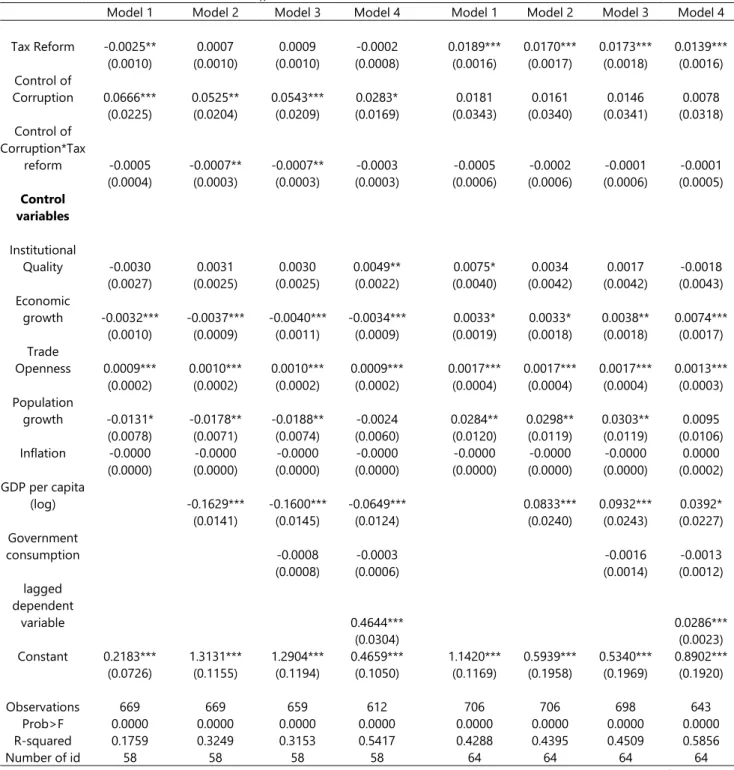
Table 1: Interaction control of corruption/Tax reform and Fiscal space, Fixed panel specifications
Dependent variable
Fiscal Space (log (1+ debt service to government revenue ratio))
Tax revenue as percent of GDP (log)
Model 1 Model 2 Model 3 Model 4 Model 1 Model 2 Model 3 Model 4
Tax Reform -0.0025** 0.0007 0.0009 -0.0002 0.0189*** 0.0170*** 0.0173*** 0.0139*** (0.0010) (0.0010) (0.0010) (0.0008) (0.0016) (0.0017) (0.0018) (0.0016) Control of Corruption 0.0666*** 0.0525** 0.0543*** 0.0283* 0.0181 0.0161 0.0146 0.0078 (0.0225) (0.0204) (0.0209) (0.0169) (0.0343) (0.0340) (0.0341) (0.0318) Control of Corruption*Tax reform -0.0005 -0.0007** -0.0007** -0.0003 -0.0005 -0.0002 -0.0001 -0.0001 (0.0004) (0.0003) (0.0003) (0.0003) (0.0006) (0.0006) (0.0006) (0.0005) Control variables Institutional Quality -0.0030 0.0031 0.0030 0.0049** 0.0075* 0.0034 0.0017 -0.0018 (0.0027) (0.0025) (0.0025) (0.0022) (0.0040) (0.0042) (0.0042) (0.0043) Economic growth -0.0032*** -0.0037*** -0.0040*** -0.0034*** 0.0033* 0.0033* 0.0038** 0.0074*** (0.0010) (0.0009) (0.0011) (0.0009) (0.0019) (0.0018) (0.0018) (0.0017) Trade Openness 0.0009*** 0.0010*** 0.0010*** 0.0009*** 0.0017*** 0.0017*** 0.0017*** 0.0013*** (0.0002) (0.0002) (0.0002) (0.0002) (0.0004) (0.0004) (0.0004) (0.0003) Population growth -0.0131* -0.0178** -0.0188** -0.0024 0.0284** 0.0298** 0.0303** 0.0095 (0.0078) (0.0071) (0.0074) (0.0060) (0.0120) (0.0119) (0.0119) (0.0106) Inflation -0.0000 -0.0000 -0.0000 -0.0000 -0.0000 -0.0000 -0.0000 0.0000 (0.0000) (0.0000) (0.0000) (0.0000) (0.0000) (0.0000) (0.0000) (0.0002) GDP per capita (log) -0.1629*** -0.1600*** -0.0649*** 0.0833*** 0.0932*** 0.0392* (0.0141) (0.0145) (0.0124) (0.0240) (0.0243) (0.0227) Government consumption -0.0008 -0.0003 -0.0016 -0.0013 (0.0008) (0.0006) (0.0014) (0.0012) lagged dependent variable 0.4644*** 0.0286*** (0.0304) (0.0023) Constant 0.2183*** 1.3131*** 1.2904*** 0.4659*** 1.1420*** 0.5939*** 0.5340*** 0.8902*** (0.0726) (0.1155) (0.1194) (0.1050) (0.1169) (0.1958) (0.1969) (0.1920) Observations 669 669 659 612 706 706 698 643 Prob>F 0.0000 0.0000 0.0000 0.0000 0.0000 0.0000 0.0000 0.0000 R-squared 0.1759 0.3249 0.3153 0.5417 0.4288 0.4395 0.4509 0.5856 Number of id 58 58 58 58 64 64 64 64
Source: Authors estimations. Standard errors in parentheses. *** p<0.01, ** p<0.05, * p<0.1. we add plus 1 to the log of debt service to revenue ratio as the minimum value of the ratio is 0.
4.2. Panel Smooth threshold regressions results
As we show in the previous section, PSTR requires to first test the hypothesis of linearity. For the regressions, we adopt the same approach as in the simple panel regressions allowing the linearity tests to discriminate about the suitable specifications. Table 2 reports the linearity tests of the final specifications only; this done in order to save space. We finally retain three specifications for each dependent variable. Especially specifications with the ratio of debt service to revenue do not include lagged dependent variable, while those with tax revenue include its lagged dependent variable. For the first dependent variable, when the lagged fiscal space variable is introduced, the tests reject the non-linear specification, or the estimates become very large which makes it difficult to give an economic interpretation. Clearly, the three tests of linearity strongly reject the null hypothesis of linearity of the relationship between tax reform and the fiscal space variables conditional to the level of control of corruption index in the six regressions. But no-remaining non-linearity tests fails to reject the null hypothesis of one regime against the alternative of at least two extreme regimes, suggesting one transition process between two extreme regimes.
Tableau 2: Linearity tests
Dependent
variable Fiscal Space (log) Tax revenue as percent of GDP (log)
Model 1 Model 2 Model 3 Model 1 Model 2 Model 3
Tests Linearity r=1 versus r=2 Linearity r=1 versus r=2 Linearity r=1 versus r=2 Linearity r=1 versus r=2 Linearity r=1 versus r=2 Linearity r=1 versus r=2 Wald Tests (LM) 68.414 13.825 30.318 9.818 33.650 14.506 16.464 11.859 17.784 12.440 22.611 13.431 p-value 0.000 0.032 0.000 0.199 0.000 0.069 0.021 0.105 0.023 0.133 0.007 0.144 Fisher Tests (LMF) 11.467 2.084 4.089 1.253 3.982 1.621 2.148 1.499 2.029 1.369 2.304 1.306 p-value 0.000 0.053 0.000 0.272 0.000 0.116 0.037 0.165 0.041 0.207 0.015 0.230 LRT Tests (LRT) 72.141 13.969 31.026 9.890 34.540 14.668 16.674 11.967 18.032 12.561 23.018 13.573 p-value 0.000 0.030 0.000 0.195 0.000 0.066 0.020 0.102 0.021 0.128 0.006 0.138
Source: authors estimations
Table 3 reports the different estimated parameters. The location parameters are relatively stable across regressions and differ between the two dependent variables. In the regressions with the burden of debt service on government revenue, the estimated thresholds are around 1.9 and 2 against 3.9 —twice as much as in the debt service burden specifications — in the regressions with tax revenue as percentage of GDP. These results suggest that controlling corruption is highly critical to improving tax revenue if a country intends to develop a sustainable fiscal space.
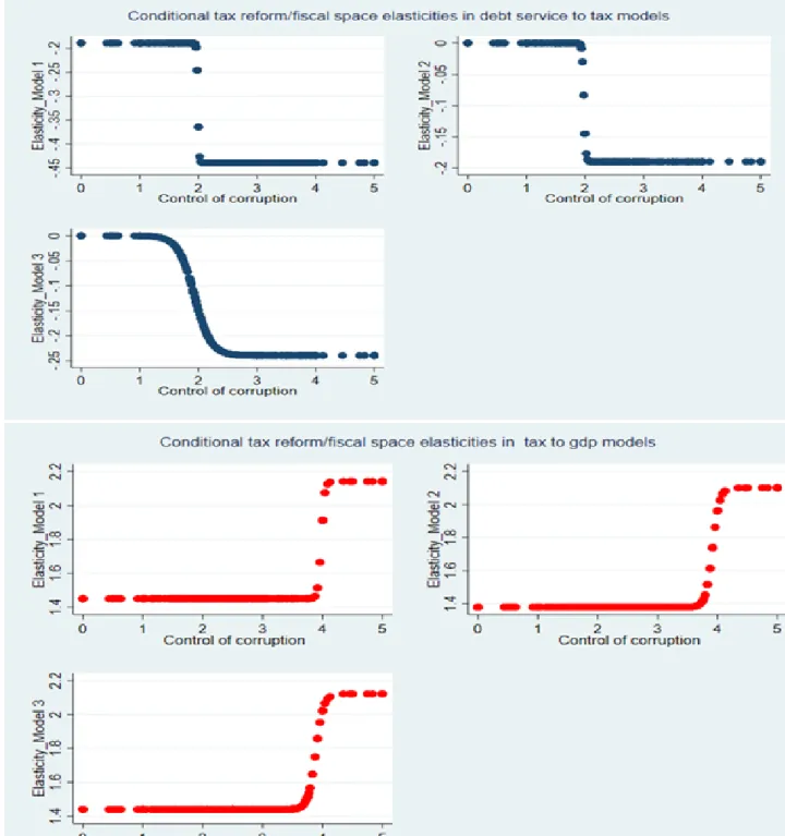
As usual in PSTR, Figure 6 plots the graphs of the tax reform elasticities of fiscal space variables against the control of corruption index for each regression. They indicate that an increase in the control of corruption— our threshold variable—is associated with a negative relationship between tax reform and debt service burden from the lower to the higher regimes. In tax to GDP models, higher level of corruption control is associated with a positive relationship between tax reform and revenue mobilization. However, the transition shape seems abrupt for the two first models in debt service to government revenue specifications while it is clearly smooth in the third model which combines all the explanatory variables. The slope parameters of the two first models— 99.35 and 68.49 respectively—are very large compared to that of the third model with 7.2 as slope parameter. Moreover, model 3 exhibits the lowest RSS —4.517 which indicates that it meets the PSTR requirements well. We can notice that the exhibited threshold is close to 2 confirming the results above. The direct effect of tax reform is only negative and statistically significant in model 1 while its interaction with the corruption control index is statistically and robustly negative across all the regressions suggesting that a minimum of control of corruption is necessary to favor the enhanced effects of tax reform on fiscal space. Consequently, we can conclude that the improvement in control of corruption is positively associated with a positive relationship between tax reform to fiscal space from lower to upper regimes. The stronger the corruption control, the higher the tax reform effect on fiscal space. We can draw a similar conclusion with the ratio of tax to GDP models. As control of corruption improves, the greater the positive tax reform effect on tax revenues. These results are consistent with the argument that the fight against corruption is important for ensuring the effectiveness of tax reform in creating fiscal space. They corroborate several studies in literature among them Ghura (1998), Attila et al. (2009), Bird et al. (2008). But they do not support findings such as those of Akdede (2011) and Alm et al. (2016) who argue that higher level of corruption can force taxpayers to comply with tax payment. This difference could be explained by the differences in samples and study period as well as by difference in econometric approaches.
With regard to the control variables, the signs and significances in PSTR are closely similar to those of the simple panel regressions. However, the PSTR estimates mostly exhibit higher estimates than those of the former regressions. The institutional quality is only statistically significant in model 1 of our first dependent variable. But its expected negative and positive signs respectively in our preferred fiscal space and tax revenue to GDP models, model 3 are statistically insignificant. Economic growth and GDP per capita strongly enter the regressions with the expected and statistically significant signs confirming that economic performances and level of development are means of boosting tax revenue and enhancing fiscal space.
Figure 6: Tax reform/fiscal space elasticities conditional on corruption control index, PSTR.
Table 3: PSTR results of estimation
Dependent
variable Fiscal Space (log) Tax revenue as percent of GDP (log)
Threshold
variable Control of corruption
Model 1 Model 2 Model 3 Model 1 Model 2 Model 3
𝛼 Tax Reform
-0.0019*** 0.0005 0.0012 0.0144*** 0.0137*** 0.0143*** (0.0009) (0.0008) (0.0009) (0.0012) (0.0013) (0.0014) 𝛽 Tax reform × 𝑓 -0.0025*** -0.0019** -0.0024*** 0.0068*** 0.0071*** 0.0067*** (0.0010) (0.0009) (0.0009) (0.0016) (0.0014) (0.0014) Loc parameter 1.9915 1.9828 1.9310 3.9805 3.9171 3.8866 Slope parameter 99.3514 68.4948 7.1669 36.1747 17.3147 15.5157 Control variables Institutional Quality -0.0113** -0.0089 -0.0059 0.0053 0.0031 0.0007 (0.0056) (0.0068) (0.0064) (0.0040) (0.0041) (0.0041) Economic growth -0.0011 -0.0023* -0.0042** 0.0074*** 0.0077*** 0.0081*** (0.0014) (0.0013) (0.0019) (0.0017) (0.0017) (0.0017) Trade Openness 0.0012* 0.0011* 0.0011* 0.0011*** 0.0011*** 0.0011*** (0.0007) (0.0006) (0.0006) (0.0003) (0.0003) (0.0003) Population growth -0.0326*** -0.0365*** -0.0450*** 0.0037 0.0076 0.0082 (0.0120) (0.0114) (0.0144) (0.0107) (0.0110) (0.0111) Inflation (Deflator) -0.0000** -0.0000 -0.0000 0.0010* 0.0013** 0.0011* (0.0000) (0.0000) (0.0000) (0.0006) (0.0006) (0.0007)GDP PPP per capita (log) -0.1446*** -0.1437*** 0.0524*** 0.0537***
(0.0153) (0.0160) (0.0214) (0.0221) Government Consumption -0.0025 -0.0015* (0.0018) (0.0009) Lagged dependent variable 0.0299*** 0.0284*** 0.0278*** (0.0035) (0.0036) (0.0036) RSS 5.535 4.583 4.517 9.179 8.951 8.731 Number of observations 669 669 659 643 643 643
Source: Author estimations. *, ** and *** denote significance at the 10, 5 and 1percent level, respectively.
That is, a one-unit increase in growth leads to a reduction in debt service to revenue ratio by 0.42 percent and an increase of 0.81 percent in tax to GDP revenue. A one unit increase of real GDP per capita translates into a decrease of about 13.4 percent decrease in debt service relative to revenue burden and by an increase of 5.52 percent in tax to GDP revenue. Trade openness alike in the linear interaction specifications presents mixed results. Its effects on the two dependent variables are strongly positive and statistically significant with fairly identical estimates. This result suggests that while trade openness deteriorates the fiscal space as measured by the burden of debt service to revenue, it equally enhances tax revenue collection. One-unit increase in trade openness is
associated with a deterioration of fiscal space and an improvement of the level of tax revenues by 0.11 percent. As we argued above, these contrasting effects are linked to the ambiguity concerning the effects of globalization on fiscal performances and are in line with the literature, although we expected that the enhancing effects would outweigh the negative effects.
Population growth enhances fiscal space as suggested by the negative and statistically significant estimate. However, it does not show any statistically significant effect on tax to GDP ratio. When considering the inflation rate, it also tends to enhance fiscal space, but its effect is not statistically significant in our preferred model 3 of debt service to tax ratio and is only significant at 10 percent in the third specification of tax to GDP model. Furthermore, general government consumption does not support the argument of the Cyan et al. (2013). The insignificance of this result could be explained by the non-inclusion of the other categories of government expenditure including investment that could exert pressure on debt and tax revenues. Lastly, the robust and significant effect at 1 percent of the lagged tax revenue on tax to GDP demonstrates that tax performances can be persistent effects.
In short, our results are broadly in line with the literature on the corruption-tax reform-fiscal space nexus. Nonetheless, our interest focuses on the signs of the tax reform parameters instead of the magnitude of its elasticities because there is a continuum of elasticities between the two regimes. As allowed by the PSTR regression, this is due to the nature of time varying and country differences effects which comes from the deviation of the observed corruption control index to the estimated threshold. Compared to the standard approach, interpreting the magnitude of the elasticities requires an additional work as shown by equation 1.2. From equation 1.2, we only compute the average estimated elasticities for all the countries in the sample and focus our analysis on a selection among them to highlight the time varying effects across countries.
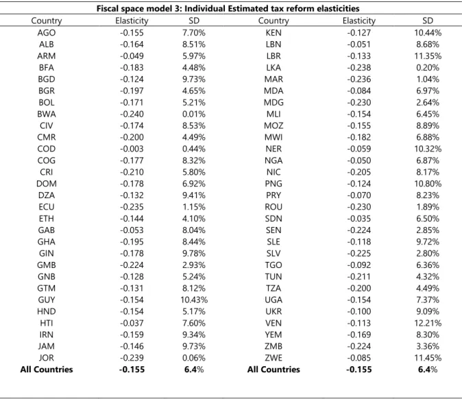
Table 4 reports the average estimated elasticities alongside their standard deviation by country respectively for the two dependent variables. For each of them, a figure that includes time varying for a selection of countries is associated. Keeping in mind that elasticities should be considered in absolute term so that higher values indicate higher effect of fiscal space. We only consider estimates from Model 3 for both dependent variables which is the optimal model as its threshold leads to the strongest rejection of the null linearity assumption. The reading of the tables showcases two key lessons. First, the response effects of fiscal space to tax reform are heterogeneous across the countries and over time, supporting our analyses above. The average corresponding tax reform
estimated elasticities are quite different from one country to another. The average estimated elasticity of fiscal space to tax reform is 0.155 in Angola, 0.174 in Cote d’Ivoire but 0.236 in Morocco, 0.1 in Ukraine and only 0.03 in Democratic Republic of Congo and 0.05 in Armenia, Gabon and Nigeria. Figure 7 demonstrates that individual elasticity varies over period. A closer comparison with section 2 shows that the estimates move erratically depending on the values of the corruption control index. Hence, the second lesson is that countries that reap most from tax reforms are those
that are able to control corruption
.
This conclusion is also confirmed by Figure 7. Regarding taxrevenue sensitivity to tax reform, similar conclusions hold although the variability is less pronounced than in the other dependent variable. This is expected as the transition slope for tax to GDP model is much higher. All these results support our econometric approach that simple linear models do not provide enough information on the accurate effects of tax reform on fiscal space and that
heterogeneity does exist across countries.In addition, we find that, regardless of the region or the
income groups to which they belong, the magnitude of the effects can vary from one country to another. For instance, because they perform well in terms of controlling corruption compared to their counterparts, the magnitude of the effects in Ghana and Senegal is higher than in Kenya, Gabon and Nigeria. Similar point can be made for Burkina Faso (BFA), Liberia (LBR) and Niger (NER). Hence, for two countries with similar incomes, tax reform may have less impact on the fiscal space in one of the countries if that country has a higher level of corruption.
Table 4: Individual Estimated tax reform elasticities
Fiscal space model 3: Individual Estimated tax reform elasticities
Country Elasticity SD Country Elasticity SD
AGO -0.155 7.70% KEN -0.127 10.44% ALB -0.164 8.51% LBN -0.051 8.68% ARM -0.049 5.97% LBR -0.133 11.35% BFA -0.183 4.48% LKA -0.238 0.20% BGD -0.124 9.73% MAR -0.236 1.04% BGR -0.197 4.65% MDA -0.084 6.97% BOL -0.171 5.21% MDG -0.230 2.64% BWA -0.240 0.01% MLI -0.154 6.45% CIV -0.174 8.53% MOZ -0.155 8.89% CMR -0.200 4.49% MWI -0.182 6.88% COD -0.003 0.44% NER -0.059 10.32% COG -0.177 8.32% NGA -0.050 6.87% CRI -0.210 5.80% NIC -0.205 8.17% DOM -0.178 6.92% PNG -0.124 10.80% DZA -0.132 9.41% PRY -0.070 8.23% ECU -0.235 1.15% ROU -0.230 1.89% ETH -0.144 4.10% SDN -0.035 6.50% GAB -0.053 8.04% SEN -0.224 2.85% GHA -0.195 8.44% SLE -0.118 9.72% GIN -0.178 9.78% SLV -0.225 2.80% GMB -0.224 2.93% TGO -0.092 6.36% GNB -0.128 5.24% TUN -0.211 4.32% GTM -0.131 8.12% TZA -0.200 4.49% GUY -0.154 10.43% UGA -0.154 7.37% HND -0.154 5.17% UKR -0.100 9.09% HTI -0.037 7.60% VEN -0.113 12.21% IRN -0.159 9.34% YEM -0.169 8.30% JAM -0.146 9.73% ZMB -0.224 3.36% JOR -0.239 0.06% ZWE -0.085 11.45%
Tax to GDP model 3: Individual Estimated tax reform elasticities
Country Elasticity SD Country Elasticity SD
AGO 1.440 0% KWT 1.440 0.0% ALB 1.518 19% LBN 1.485 16.1% ARM 1.440 0% LBR 1.440 0.0% BFA 1.485 16% LKA 1.527 19.0% BGD 1.440 0% MAR 1.440 0.0% BGR 1.633 30% MDA 1.440 0.0% BHS 1.940 22% MDG 1.859 26.0% BOL 1.440 0% MLI 1.440 0.0% BRN 1.640 31% MOZ 1.664 29.4% BWA 1.501 19% MWI 1.446 2.0% CIV 1.530 22% NAM 1.593 29.1% CMR 1.444 2% NER 1.440 0.0% COG 1.530 22% NGA 1.440 0.0% CRI 1.755 35% NIC 1.711 32.8% DOM 1.503 17% PAN 1.440 0.0% DZA 1.480 14% PNG 1.441 0.1% ECU 1.440 0% PRY 1.440 0.0% ETH 1.440 0% ROU 1.535 21.7% GAB 1.440 0% SDN 1.440 0.0% GHA 1.446 2% SEN 1.440 0.0% GIN 1.578 25% SLE 1.440 0.0% GMB 1.440 0% SLV 1.509 17.6% GNB 1.440 0% SUR 1.440 0.0% GTM 1.517 19% TGO 1.440 0.0% GUY 1.440 0% TUN 1.440 0.0% HND 1.440 0% TZA 1.574 25.5% HRV 1.440 0% UGA 1.440 0.0% HTI 1.440 0% UKR 1.440 0.0% IRN 1.575 25% VEN 1.440 0.0% JAM 1.440 0% YEM 1.440 0.0% JOR 1.575 25% ZMB 1.485 16.1% KEN 1.440 0% ZWE 1.530 21.8%
All Countries 1.500 9% All Countries 1.500 9.4%
Figure 8: Heterogenous and individual time varying tax reform elasticities
Conclusion
This paper assesses the effects of tax reform on fiscal space conditional to the level of corruption control for a large panel of developing and emerging economies over 1990-2016. A number of papers have demonstrated that corruption can hinder the efforts of governments to increase their public revenues and fiscal space. We use the debt service to total government revenue and tax to GDP revenue ratios as fiscal space variables while tax reform is modelled by an index of tax structure similar to that of the advanced economies. Using a threshold approach, our findings indicate that tax reform’s effect on fiscal space is not monotonic and depends on corruption control. Tax reform enhances fiscal space and tax revenue when corruption control is improved. They also suggest that heterogeneity across countries and time do matter. We then provide an estimation of elasticities to tax reform of fiscal space variables for each country and period. This confirms that countries that benefit most from tax reforms are those that prove enough ability to control corruption irrespective of the regions they belong to.
These results have strong policy implications for tax reforms designed towards expanding a country’s fiscal space. They suggest that controlling corruption and improving the quality of policies that help control it are central to support the effectiveness of tax reforms. The fact that some countries show some downward trend despite commitments made to fight corruption suggest that stronger effective efforts are still necessary. Therefore, countries and their partners must step-up their joint efforts towards the reinforcement of actions, reforms and framework against corruption. However, our results suggest that tailored policies will ensure effective outcomes depending on the level of corruption and the institutional environment of each country. Reforms priorities could differ across countries and over time.
References
Acemoglu, D., & Robinson, J. A. (1999). On the political economy of institutions and development. American Economic Review, 91(4), 938-63.
Acemoglu, D., Johnson, S., & Robinson, J. A. (2005). Institutions as a fundamental cause of long-run growth. Handbook of economic growth, 1, 385-472.
Ades, A., & R. Di Tella (1997). National Champions and Corruption: Some Unpleasant Interventionist Arithmetic. Economic Journal vol.107, n° 443, pp. 1023-43.
Agbeyegbe, T. D., Stotsky, J., & WoldeMariam, A. (2006). Trade liberalization, exchange rate changes, and tax revenue in Sub-Saharan Africa. Journal of Asian Economics, 17(2), 261-284.
Akdede, S. H. (2011). Corruption and tax evasion. Doğuş Üniversitesi Dergisi, 7(2), 141-149.
Alm, J., Martinez-Vazquez, J., & McClellan, C. (2016). Corruption and firm tax evasion. Journal of
Economic Behavior & Organization, 124, 146-163.
Attila, G., Chambas, G., & Combes, J. L. (2009). Corruption et mobilisation des recettes publiques : une analyse économétrique. Recherches Economiques De Louvain/Louvain Economic Review, 75(2), 229-268.
Aizenman, J., & Jinjarak, Y. (2010). De Facto Fiscal Space and Fiscal Stimulus: Definition and Assessment. NBER Working Paper, (w16539).
Aizenman, J., Jinjarak, Y., Nguyen, H. T. K., & Park, D. (2019). Fiscal space and government-spending and tax-rate cyclicality patterns: A cross-country comparison, 1960–2016. Journal of
Macroeconomics, 60, 229-252.
Baum, A., Gupta, S., Kimani, E., & Tapsoba, S. J. (2017). Corruption, taxes and compliance. eJournal
of Tax Research, 15(2), 190-216.
Béreau S., Villavicencio A. L., Mignon V. (2012) ‘Currency Misalignments and Growth: A New Look Using Nonlinear Panel Data Methods’, Applied Economics, 44: 3503–11.
Bird, R. M., Martinez-Vazquez, J., & Torgler, B. (2008). Tax effort in developing countries and high income countries: The impact of corruption, voice and accountability. Economic analysis and
policy, 38(1), 55-71.
Bird, R. M., Martinez-Vazquez, J., & Torgler, B. (2014). Societal institutions and tax effort in developing countries. Annals of Economics and Finance, 15(1), 185-230.
Bray, J. R., & Curtis, J. T. (1957). An ordination of the upland forest communities of Southern Wisconsin. Ecological Monographies, 27, 325–34
Brun, J. F., Chambas, G., & Mansour, M. (2015). Tax effort of developing countries: An alternative measure. Financing sustainable development addressing vulnerabilities, 205-216.