Enumeration of polyominoes defined in terms of pattern avoidance or convexity constraints

(1)

HAL Id: tel-01064960

https://tel.archives-ouvertes.fr/tel-01064960

Submitted on 17 Sep 2014

HAL is a multi-disciplinary open access

archive for the deposit and dissemination of sci-entific research documents, whether they are pub-lished or not. The documents may come from

L’archive ouverte pluridisciplinaire HAL, est destinée au dépôt et à la diffusion de documents scientifiques de niveau recherche, publiés ou non, émanant des établissements d’enseignement et de

Enumeration of polyominoes defined in terms of pattern

avoidance or convexity constraints

Daniela Battaglino

To cite this version:

Daniela Battaglino. Enumeration of polyominoes defined in terms of pattern avoidance or convexity constraints. Other [cs.OH]. Université Nice Sophia Antipolis, 2014. English. �NNT : 2014NICE4042�. �tel-01064960�

(2)

Enumeration of polyominoes deined in

terms of pattern avoidance or convexity

constraints

Thesis of the University of Siena and the University of Nice Sophia Antipolis

Advisors: Prof. Simone Rinaldi and Prof. Jean Marc Fédou to obtain the

Ph.D. in Mathematical Logic, Informatics and Bioinformatics of the University of Siena

Ph.D. in Information and Communication Sciences of the University of Nice Sophia Antipolis

Candidate: Daniela Battaglino Siena, June 26th, 2014 Jury composed by:

Prof. Elena Barcucci Prof. Marilena Barnabei Prof. Srečko Brlek Prof. Enrica Duchi Prof. Jean Marc Fédou Prof. Rinaldi Simone

(3)

CONTENTS CONTENTS 3.3.2 Robust polyomino classes . . . 79 3.4 Some families of permutations deined by submatrix avoidance 82 3.4.1 Generalised permutation patterns . . . 83 3.4.2 A diferent look at some known permutation classes . . 84 3.4.3 Propagating enumeration results . . . 87 3.5 Some families of polyominoes deined by submatrix avoidance 88 3.5.1 Characterisation of known families of polyominoes . . . 88 3.6 Generalised pattern avoidance . . . 92 3.7 Deining new families of polyominoes by submatrix avoidance . 97 3.8 Some directions for future research . . . 103

(5)

Introduction

This dissertation discusses some topics and applications in combinatorics. Combinatorics is a branch of mathematics which concerns the study of families of discrete objects which are often designed as models for real ob-jects. The motivations for studying these objects may arise from informatics (models for data structures, analysis of algorithms, ...), but also from biology - in particular molecular and evolutive biology [58] - from physics as in [13] or from chemistry [31].

Combinatorialists are particularly interested in several aspects of a fam-ily of objects: its diferent characterisations, the description of its properties, the enumeration of its elements, and their generation both randomly or ex-haustively, by the use of algorithms, the deinition of some relations (as for example order relations) between the elements belonging to the same family. We have taken into consideration two remarkable subields of combinatorics, which have often been considered in the literature. These two aspects are closely related, and they give a deep insight on the nature of the combinato-rial structures which are being studied: enumerative combinatorics and the study of patterns into combinatorial structures.

Enumerative Combinatorics. An unavoidable step for understanding the structure of a family of objects is certainly the capability of counting its elements. Among the many ways of describing sets of objects, the list of its elements is the basic one and convenient for inite and small sets. For larger sets this is obviously problematic, and mathematicians developed this ield in several directions in order to “understand” the meaning of their observations. Recently in the history of mankind, enumerative combinatorics emerged as a powerful tool. As enumerative combinatorics deal with inite families of objects, it is convenient to look for bijections with inite subsets of integers, in other words counting the number of its elements in an exact way if possible, and approximate otherwise. Various problems arising from diferent ields can be solved by analysing them from a combinatorial point of view. Usually, these problems have the common feature to be represented by simple objects suitable to enumerative techniques of combinatorics. Given

(6)

a family O of objects and a parameter � on this family, called the size, we focus on the set On of objects for which the value of the parameter is equal to �, where � is a nonnegative integer. The parameter � is discriminating if, for each non negative integer �, the number of objects of On is inite. Then, we ask for the cardinality �n of the set On for each possible �. Enumerative combinatorics answers to this question. Only in rare cases the answer will be a completely explicit closed formula for �n, involving only well known functions, and free from summation symbols. However, a recurrence for �n may be given in terms of previously calculated values �k, thereby giving a simple procedure for calculating �n for any � ∈ N. Another approach is based on generating functions: whether we do not have a simple formula for �n, we can hope to get one for the formal power series �(�) = �n�n�n, which is called the generating function of the family O according to the parameter �. Notice that the �-th coeicient of the Taylor series of �(�) is just the term �n. In some cases, once that the generating function is known, we can apply standard techniques in order to obtain the required coeicients �n(see for instance [79, 82]). Otherwise we can obtain an asymptotic value of the coeicients through the analysis of the singularities in the generating function (see [69]).

Several methods for the enumeration, using algebraic or analytical tools, have been developed in the last forty years. A irst general and empirical approach consists in calculating the irst terms of �n and then try to deduce the sequence. For instance, one can use the book by Sloane and Ploufe [103, 114] in order to compare the irst numbers of the sequence with some known sequences and try to identify �n. More advanced techniques (Brak and Guttmann [32]) start from the irst terms of the sequence and ind an algebraic or diferential equation satisied by the generating function of the sequence itself. A more common approach consists in looking for a construc-tion of the studied family of objects and successively translating it into a recursive relation or an equation, usually called functional equation, satisied by the generating function �(�). The approach to enumeration of combina-torial objects by means of generating functions has been widely used (see for instance Goulden and Jackson [79] and Wilf [125]). Another technique which has often been applied to solve combinatorial problems is the Schützen-berger methodology, also called DSV [112], which can be decomposed into three steps. The irst one consists in constructing a bijection between the objects and the words of an algebraic language in such a way that for every object the parameter to the length of the words of the language. At the next step, if the language is generated by an unambiguous context-free grammar, then it is possible to translate the productions of the grammar into a sys-tem of functional equations. Finally one deduces an equation for which the

(7)

generating function of the sequence �n is the unique and algebraic solution (Schützenberger and Chomsky [44]). A variant of the DSV methodology are the operator grammars (Cori and Richard [51]). These grammars take in account some cases in which the language encoding the objects is not alge-braic. The theory of combinatorial species described by Joyal [89], is the irst unifying presentation of a combinatorial theory of formal power series, where operations on species relect on the generating functions and vice versa. A comprehensive exposition can be found in Bergeron, Labelle and Leroux [16], with numerous examples: arithmetic operations on power series cor-respond to natural transformations on species, building a powerful calculus for the decomposition or substitution in species. A variant is the theory of decomposable structures (Flajolet, Salvy, and Zimmermann [67, 68]), which also describes recursively the objects in terms of basic operations between them. These operations are directly translated into operations between the corresponding generating functions, cutting of the passage to words. A nice presentation of this theory appears in the book of Flajolet and Sedgewick [69]. An elegant formalization of decomposable structures was introduced in [62] by Dutour and Fédou: it is based on the notion of object grammars and describe objects using very general operators.

A signiicantly diferent way of recursively describing objects appears in the ECO methodology, introduced by Barcucci, Del Lungo, Pergola, and Pinzani [9]. In the ECO method each object is obtained from a smaller object by making some local expansions. Usually these local expansions are very regular and can be described in a simple way by a succession rule. Then a succession rule can be translated into a functional equation for the generating function. It has been shown that this method is very efective on large number of combinatorial structures. Succession rules (under the name of generating trees) had however been applied to enumeration problems, previously [9], in [45] and [123]. We also cite [8] in which we ind an analysis of the links between the structural properties of the generating trees and the rationality, algebraicity, or transcendence of the corresponding generating function.

Another approach is to ind a bijection between the studied family of ob-jects and another one, simpler to count. In order to have consistent enumer-ative results, the bijection has to preserve the size of the objects. Moreover, a bijective approach also permits a better comprehension of some properties of the studied family and to relate them to the family in bijection with it.

Patterns in combinatorial structures. A possible strategy to under-stand more about the nature of some combinatorial structures and which provides a diferent way to look at a combinatorial object, is to describe it by the containment or avoidance of some given substructures, which are com-monly known as patterns. The concept of pattern within a combinatorial

(8)

structure is central in combinatorics. It has been deeply studied for permu-tations, starting irst with [98]. More precisely, given a permutation � we can say that � contains a certain pattern � if such a pattern can be seen as a sort of “subpermutation” of �. If � does not contain � we say that � avoids �.

In particular, the concept of pattern containment on the set of all per-mutations can be seen as a partial order relation, and it was used to deine permutation classes, i.e. families of permutations downward closed under such pattern containment relation. So, every permutation class can be de-ined in terms of a set of avoided patterns, and the minimal of this sets is called the basis of the permutation class.

These permutation classes can then be regarded as objects to be counted. We can ind many results concerning this research guideline in the literature. For instance, we quote two works that collect a large part of the obtained results. The irst is the thesis of Guibert [83] and the second is the work of Kitaev and Mansour [93]. In the second, in addition to the list of the obtained results regarding the enumeration of set of permutations that avoid a set of patterns, the authors also take into account the study of the number of objects containing a ixed number of occurrences of a certain pattern and make an interesting parallel between the concept of pattern on the set of permutations and the concept of pattern on the set of words.

Concerning the results obtained on the enumeration of classes avoiding patterns of small size, we mention the work of Simion and Schmidt [113], in which we can ind an exhaustive study of all cases with patterns of length less than or equal to three. However, for results concerning patterns of size four we refer the reader to the work of Bóna [22]. Another remarkable work of Bóna is [24], in which he studies the expected number of occurrences of a given pattern in permutations that avoid another given pattern. One of the most important recent contributions is the one by Marcus and Tardos [101], consisting in the proof of the so-called Stanley-Wilf conjecture, thus deining an exponential upper bound to the number of permutations avoiding any given pattern. Later, given the enormous interest in this area, not only patterns by the classical deinition were taken into consideration, but also patterns deined under the imposition of some constraints.

Babson and Steingrímsson [7] introduced the notion of generalised pat-terns, which requires that two adjacent letters in a pattern must be adjacent in the permutation. The authors introduced such patterns to classify the family of Mahonian permutation statistics, which are uniformly distributed with the number of inversions. Several results on the enumeration of per-mutation classes avoiding generalised patterns have been achieved. Claesson obtained the enumeration of permutations avoiding a generalised pattern of

(9)

length three [46] and the enumeration of permutations avoiding two gener-alised patterns of length three [48]. Another result in terms of permutations avoiding a set of generalised patterns of length three was obtained by Bernini et al. in [17, 18], where one can ind the enumeration of permutation avoiding set of generalised patterns as a function of its length and another parameter. Another kind of patterns, called bivincular patterns, was introduced in [26] with the aim to increase the symmetries of the classical patterns. A bijection between permutations avoiding a particular bivincular pattern was derived, as well as several other families of combinatorial objects. Finally, we mention the mesh patterns, which were introduced in [34] to generalise several varieties of permutation patterns.

Otherwise, from the algorithmic point of view, a challenging problem is to ind an eicient way to establish whether an element belongs to a per-mutation class C. More precisely, if we know the elements of the basis of C, and especially if the basis is inite, this problem consists in verifying if a permutation contains an element of the basis. Generally the complexity of the algorithms is high, but there are some special cases in which linear algorithms have been found, for instance in [98].

Another remarkable problem is to calculate the basis of a given permuta-tion class. A very useful result in this direcpermuta-tion was obtained by Albert and Atkinson in [1], namely a necessary and suicient condition to ensure that a permutation class has a inite basis.

As we have previously mentioned, some deinitions analogous to those given for permutations were provided in the context of many other com-binatorial structures, such as set partitions [81, 97, 111], words [20, 35], trees [52, 60, 70, 73, 91, 105, 109, 118], and paths [19].

In the present thesis we examine the two previously quoted general issues, on a rather remarkable family of combinatorial objects, i.e. the polyominoes. These objects arise in many scientiic areas of research, for instance in combi-natorics, physics, chemistry,... (more explicit details are given in Chapter 1). In particular, in this thesis, we consider under a combinatorial and an enu-merative point of view families of polyominoes deined by imposing several types of constraints.

The irst type of constraint, which extends the well-known convexity con-straint [57], is the �-convexity concon-straint, introduced by Castiglione and Restivo [40]. A convex polyomino is said to be �-convex if every pair of its cells can be connected by a monotone path with at most � changes of di-rection. The problem of enumerating �-convex polyominoes was solved only for the cases � = 1, 2 (see [38, 61]), while the case � > 2 is yet open and seems

(10)

diicult to solve. To address it, we have investigated a particular subfamily of �-convex polyominoes, the �-parallelogram polyominoes, i.e. the �-convex polyominoes that are also parallelogram.

The second type of constraint extends, in a natural way, the concept of pattern avoidance on the set of polyominoes. Since a polyomino can be represented as a binary matrix, we can say that a polyomino � is a pattern of a polyomino � when the binary matrix representing � is a submatrix of that representing �. Our attempt is to reconsider the problems treated within permutation classes for the case of pattern avoiding polyominoes.

Using this idea, we have deined a polyomino class to be a set of polyomi-noes which are downward closed w.r.t. the containment order. Then we have given a characterisation of some known families of polyominoes, using this new notion of pattern avoidance. This new approach also allowed us to study a new deinition of permutations that avoid submatrices, and to compare it with the classical notion of pattern avoidance.

In details, the thesis is organized as follows.

Chapter 1 provides the basic deinitions of the most important combi-natorial structures considered in the thesis and contains a brief state of the art. In this work we study three main families of objects. The irst one is the family of �-parallelogram polyominoes, studied from an enumerative viewpoint. The second one is the family of permutations: in particular we present the concept of patterns avoidance. The third and last family we have focused on is the one of partially ordered sets (p.o.sets or simply posets).

In Chapter 2, we deal with the problem of enumerating the subfamily of �-parallelogram polyominoes. More precisely we provide an unambiguous decomposition for the family of the �-parallelogram polyominoes, for any � ≥ 1. Then, we also translate this decomposition into a functional equa-tion satisied by their generating funcequa-tion for any �. We are then able to express such a generating function in terms of the Fibonacci polynomials and thanks to this new expression we ind a bijection between the family of �-parallelogram polyominoes and the family of rooted plane trees having height less than or equal to � + 2.

In Chapter 3 we study the concept of pattern avoidance on sets of permu-tations and polyominoes both seen as matrices. In particular, this approach allows us to deine these classes of objects as the sets of elements that are downward closed under the pattern relation, that is a partial order relation. We then study the poset of polyominoes, from an algebraic and a combinato-rial viewpoint. Moreover, we introduce several notions of bases, and we study the relations among these. We investigate families of polyominoes described by the avoidance of matrices, and families which are not. In this latter case, we consider some possible extensions of the concept of submatrix avoidance

(11)

(12)

Chapter 1 Polyominoes, permutations and

posets

This thesis studies the combinatorial and enumerative properties of some families of polyominoes, deined in terms of particular constraints of convexity and connectivity. Before we discuss these concepts in depth, we need to summarise the main deinitions and classiications of polyominoes. More speciically, we introduce the notions of polyomino, permutation and posets (partially ordered set). The chapter is organised as follows. In Section 1.1 we briely introduce the history of polyominoes; in Section 1.2 we discuss some of the most important families of polyominoes; in Section 1.3 we focus on permutations; Section 1.4 concludes the chapter by discussing posets.

1.1 Polyominoes

The enumeration of polyominoes on a regular lattice is one of the most studied topics in Combinatorics. The term polyomino was introduced by Golomb in 1953 during a talk at the Harvard Mathematics Club (which was published one year later [80]) and popularized by Gardner in 1957 [74]. A polyomino is deined as follows.

Deinition 1. In the plane Z × Z a cell is a unit square and a polyomino is a inite connected union of cells having no cut point.

Polyominoes are deined up to translations. Polyominoes can be similarly deined in other two-dimensional lattices (e.g. triangular or honeycomb); however, in this work we will focus exclusively on the square lattice.

A column (resp. row) of a polyomino is the intersection between the polyomino and an ininite strip of cells whose centers lie on a vertical (resp.

(13)

horizontal) line. A polyomino is often studied with respect to the following four parameters: area, width, height and perimeter. The area is the number of elementary cells of the polyomino; the width and height are respectively the number of columns and rows; the perimeter is the length of the polyomino’s boundary.

As we already observed, polyominoes have been studied for a long time in Combinatorics, but they have also drawn the attention of physicists and chemists. The former in particular established a relationship with polyomi-noes by deining equivalent objects named animals [59, 84], obtained by tak-ing the center of the cells of a polyomino as shown in Figure 1.1. These models allowed to simplify the description of phenomena like phase transi-tions (Temperley, 1956 [120]) or percolation (Hammersely, [85]).

(a) (b)

Figure 1.1: A polyomino in (�) and the corresponding animal in (�). Other important problems concerned with polyominoes are the problem of covering a polyomino with rectangles [41] or problems of tiling regions by polyominoes [15, 50].

In this work we are mostly interested in the problem enumerating poly-ominoes with respect to the area or perimeter. Several important results were obtained in the past in this ield. For example, in [95] Klarner proved that, given �n polyominoes of area �, the limit

lim n→∞�

1 n n

tends to a growth constant � such that: 3.72 < � < 4.64 .

Moreover, in 1995 Conway and Guttmann [49] adapted a method previously used for polygons to calculate �n for � ≤ 25. Further reinements by Jensen

(14)

and Guttman [87] and Jensen [88] allowed to reach respectively � = 46 and � = 56. Despite these important results, the enumeration of general polyominoes still represents an open problem whose solution is not trivial but can be simpliied, at least for certain families of polyominoes, by introducing some constraints such as convexity and directedness.

1.2 Some families of polyominoes

In this section we briely summarize the basic deinitions concerning some families of convex polyominoes. More speciically, we focus on the enu-meration with respect to the number of columns and/or rows, to the semi-perimeter and to the area. Given a polyomino � we denote with:

1. �(� ) the area of � and with � the corresponding variable;

2. �(� ) the semi-perimeter of � and with � the corresponding variable; 3. �(� ) the number of columns (width) of � and with � the corresponding

variable;

4. ℎ(� ) the number of rows (height) of � and with � the corresponding variable.

Deinition 2. A polyomino is said to be column-convex (row-convex) when its intersection with any vertical (horizontal) line is connected.

Examples of column-convex and row-convex polyominoes are provided in Figure 1.2 (�) and (�).

(c) (b)

(a)

Figure 1.2: (�): A column-convex polyomino; (�): A row-convex polyomino; (�): A convex polyomino.

(15)

In [120], Temperley proved that the generating function of column-convex polyominoes with respect to the perimeter is algebraic and established the following expression according to the number of columns and to the area:

� (�, �) = ��(1− �)

3

(1_{− �)}4_{− ��(1 − �)}2_{(1 + �)}_{− �}2_�3 . (1.1) Inspired by this work, similar results were obtained in 1964 by Klarner [95] and in 1988 by Delest [55]. The former was able to deine the generating function of column-convex polyominoes according to the area, by means of a combinatorial interpretation of a Fredholm integral; the latter derived the expression for the generating function of column-convex polyominoes as a function of the area and the number of columns, by means of the Schützem-berger methodology [44].

In the same years, Delest [55] derived the generating function for column-convex polyominoes according to the semi-perimeter by means of context-free languages and using the computer software for algebra MACSYMA1_{. Such} function is deined as follows:

� (�) = (1_{− �)} ⎛ ⎜ ⎜ ⎝ 1₋ 2 √ 2 3√2− ︂ 1 + � +︁(t2−6t+1)(1+t)_(1−t)2 2 ⎞ ⎟ ⎟ ⎠ . (1.2)

In Equation (1.2), the number of column-convex polyominoes with semi-perimeter �+2 is the coeicient of �n_{in �(�); these coeicients are an instance} of sequence �005435 [103], whose irst few terms are:

1, 2, 7, 28, 122, 558, 2641, 12822,· · · ,

and they count, for example, the number of permutations avoiding 13 − 2 that contain the pattern 23 − 1 exactly twice, but there is no combinatorial explanation of this fact. Several studies were carried out in an attempt to improve the above formulation or to obtain a closed expression not relying on software, including: a generalisation by Lin and Chang [43]; an alternative proof by Feretić [66]; an equivalent result obtained by means of Temperley’s methodology and the Mathematica software2 _{by Brak et al. [33].}

Deinition 3. A polyomino is convex if it is both column and row convex.

1_{Macsyma (Project MAC’s SYmbolic MAnipulator) is a computer algebra system that}

was originally developed from 1968 to 1982.

(16)

It is worth noting that the semi-perimeter of a convex polyomino is equiv-alent to the sum of its rows and columns (see Figure 1.2 (�)).

Bousquet-Mélou derived several expressions for the generating function of convex polyominoes according to the area, the number of rows and columns, among which we cite the one obtained in collaboration with Fédou [27] and the one in [25].

The generating function for convex polyominoes indexed by semi-perimeter obtained by Delest and Viennot in 1984 [57] is the following:

� (�) = �

2₍₁_{− 8� + 21�}2_{− 19�}3_{+ 4�}4₎

(1_{− 2�)(1 − 4�)}2 −

2�4

(1− 4�)√1− 4�. (1.3) The above expression is obtained by subtracting two series with positive terms, whose combinatorial interpretation was given by Bousquet-Mélou and Guttmann in [28]. The closed formula for the convex polyominoes is:

�n+2 = (2� + 11)4n− 4(2� + 1) ︂2�

� ︂

, (1.4)

with � ≥ 0, �0 = 1 and �1 = 2. Note that this is an instance of sequence �005436 [103], whose irst few terms are:

1, 2, 7, 28, 120, 528, 2344, 10416,_{· · · .}

In [43], Lin and Chang derived the generating function for the number of convex polyominoes with � + 1 columns and � + 1 rows, where �, � ≥ 0. Starting from their work, Gessel [76] was able to infer that the number of such polyominoes is:

� + � + �� + � ︂2� + 2� 2� ︂ − 2(� + �)︂� + � − 1 � ︂︂� + � − 1 � ︂ . (1.5)

Finally, in [54] the authors obtained the generating function of convex polyominoes according to the semi-perimeter using the ECO method [9]. Deinition 4. A polyomino � is said to be directed convex when every cell of � can be reached from a distinguished cell, called source (usually the leftmost cell at the lowest ordinate), by a path which is contained in � and uses only north and east unit steps.

(17)

(a) (b) (c) (d)

Figure 1.3: (�): A Ferrer diagram; (�): A stack polyomino; (�): A paral-lelogram polyomino; (�): A directed convex polyomino which is neither a parallelogram nor a stack one.

The number of directed convex polyominoes with semi-perimeter � + 2 is equal to �n−2, where �n is the central binomial coeicients:

�n= ︂2�

� ︂

, giving an instance of sequence �000984 [103].

The enumeration with respect to the semi-perimeter of this set was irst obtained by Lin and Chang in 1988 [43] as follows:

� (�) = �

2 √

1− 4�. (1.6)

Furthermore, the generating function of directed convex polyominoes ac-cording to the area and the number of columns and rows, was derived by M. Bousquet-Mélou and X. G. Viennot [29]:

� (�, �, �) = ��1 �0 (1.7) where �1 = ︁ n≥1 �n_�n (��)n n−1 ︁ m=0 (₋₁₎m_�(m₂) (�)m(��m+1)n−m−1 (1.8) and �0 = ︁ n≥0 (−1)n_�n_�(n+1₂ ) (�)n(��)n , (1.9) with (�)n= (�; �)n= ︀n−1 i=0(1− ��i).

(18)

Deinitions of polyominoes according to cells

It is also possible to discriminate between diferent families of polyominoes by looking at the sets of cells �, �, � and � uniquely deined by a convex polyomino and its minimal bounding rectangle, i.e. the minimum rectangle that contains the polyomino itself (see Figure 1.4). For instance, a polyomino � is directed convex when � is empty i.e., the lowest leftmost vertex belongs to � .

A B

C D

Figure 1.4: A convex polyomino and the 4 sets of cells identiied by its intersection with the minimal bounding rectangle.

In this thesis we consider the following families of polyominoes: (a) Ferrer diagram, i.e. �, � and � empty;

(b) Stack polyomino,i.e. � and � empty;

(c) Parallelogram polyomino, i.e. � and � empty.

We now review the most important results concerning the enumeration of the aforementioned sets of polyominoes.

(a) Ferrer diagrams (Figure 1.3 (�)) provide a graphical representation of integers partitions. The generating function with respect to the area, that was already known by Euler [64], is:

� (�) = 1

(�)_∞, (1.10)

while the generating function according to the number of columns and rows is:

� (�, �) = ��

1− � − �. (1.11)

The generating function of the Ferrer diagrams with respect to the semi-perimeter can be easily derived by setting all the variables of Equation (1.11)

(19)

equal to �.

(b) Stack polyominoes (Figure 1.3 (�)) can be seen as a composition of two Ferrer diagrams. Their generating function according to the number of columns, rows and area, is [126]:

� (�, �, �) =︁ n≥1

��n_�n (��)n−1(��)n

. (1.12)

The generating function with respect to semi-perimeter is rational [57]: � (�) = � 2₍₁_{− �)} 1− 3� + �2 = ︁ n≥2 �_2n−4�n, (1.13)

where �n denotes the �th number of Fibonacci. For more details on the sequence of Fibonacci �000045 the reader is referred to [103]. By deinition, the irst two numbers of the Fibonacci sequence are �0 = 0 and �1 = 1, and each subsequent number is the sum of the previous two. Consequently, their recurrence relation can be expressed as follows:

�n = �n−1+ �n−2 with � ≥ 2 . (1.14)

(c) Parallelogram polyominoes (Figure 1.3 (�)) are a particular family of convex polyominoes uniquely identiied by a pair of paths consisting only of north and east steps, such that the paths are disjoint except at their common ending points. The path beginning with a north (respectively east) step is called upper (respectively lower) path.

It is known from [116] that the number of parallelogram polyominoes with semi-perimeter � ≥ 2 is equal to the (�−1)-th Catalan number. The sequence of Catalan numbers is widely used in several combinatorial problems across diverse scientiic areas, including Mathematical Physics, Computational Bi-ology and Computer Science. This sequence of integers was introduced in the 18�ℎ Century by Leonhard Euler in an attempt to determine the diferent ways to divide a polygon into triangles. The sequence is named after the Belgian mathematician Eugène Charles Catalan, who discovered the connec-tion with the parenthesised expression of the Towers of Hanoi puzzle. Each number of the sequence is obtained as follows3_:

�n= 1 � + 1 ︂2� � ︂ .

3_{More in-depth information on the Catalan sequence A000108 is provided in [103].}

The reader may also refer to the book by R. P. Stanley [116], where over 100 diferent interpretations of Catalan numbers addressing various counting problems are provided.

(20)

The generating function of parallelogram polyominoes with respect to the number of columns and rows is:

� (�, �) = 1− � − � −︀�

2_{+ �}2_{− 2� − 2� − 2�� + 1}

2 . (1.15)

The corresponding function depending on the semi-perimeter is straightfor-wardly derived by setting all the variables equal to �. It is also worth noting that the function in Equation (1.15) is algebraic.

Delest and Fédou [56] enumerated this set of polyominoes according to the area by generalising the results of Klarner and Rivest [96] as follows:

� (�) = �1 �0 , (1.16) where: �1 = ︁ n≥1 (−1)n−1_�n_�(n+1₂ ) (�)_n−1(��)n (1.17) and �0 is the same of Equation (1.9).

1.2.1 �-convex polyominoes

The studies of Castiglione and Restivo [40] pushed the interest of the research community towards the characterisation of the convex polyominoes whose internal paths satisfy speciic constraints. We recall the following deinition of internal path of a polyomino.

Deinition 5. A path in a polyomino is a self-avoiding sequence of unit steps of four types: north � = (0, 1), south � = (0, −1), east � = (1, 0), and west � = (−1, 0), entirely contained in the polyomino.

A path connecting two distinct cells � and � of the polyomino starts from the center of �, and ends at the center of � as shown in Figure 1.5. We say that a path is monotone if it consists only of two types of steps, as in Figure 1.5 (�). Given a path � = �1. . . �k, each pair of steps �i�i+1 such that �i ̸= �i+1 , 0 < � < �, is called a change of direction.

In [40], it has been observed that in convex polyominoes each pair of cells is connected by a monotone path; therefore, a classiication of convex poly-ominoes based on the number of changes of direction in the paths connecting any two cells of the polyomino was proposed.

Deinition 6. A convex polyomino � is said to be �-convex if every pair of its cells can be connected by a monotone path with at most � changes of direction. The minimal ℎ ≥ 0 such that � is ℎ-convex is referred to as the convexity degree of � .

(21)

(a) (b)

Figure 1.5: (�): A path between two cells of the polyomino ; (�): A monotone path between two cells of the polyomino with four changes of direction.

For � = 1, we have the �-convex polyominoes, where any two cells can be connected by a path with at most one direction change. Such objects can also be characterised by means of their maximal rectangles.

Deinition 7. Let [�, �] be a rectangular polyomino with � rows and � columns, for every �, � ≥ 1. For any polyomino � we say that [�, �] is a maximal rect-angle in � if

∀ [�′_{, �}′_], _{[�, �]}_{⊆ [�}′_{, �}′_] _then _{[�, �] = [�}′_{, �}′_{] .}

Deinition 8. Two rectangles [�, �] and [�′_{, �}′_] contained in a polyomino � have a crossing intersection if their intersection is a non-trivial rectangle whose basis is the smallest of the two bases and whose height is the smallest of the two heights, i.e.

[�, �]_{∩ [�}′_{, �}′_{] = [min(�, �}′_{), min(�, �}′_{)] .}

Some examples of rectangles having non-crossing and crossing intersec-tions are shown in Figure 1.6.

Proposition 9. A convex polyomino � is �-convex if and only if any two of its maximal rectangles have a nonempty crossing intersection.

In recent literature, several aspects of the �-convex polyominoes have been studied: in [39], it has been shown that they are a well-ordering ac-cording to the sub-picture order; in [36], �-convex polyominoes are uniquely determined by their horizontal and vertical projections; inally, in [37, 38] the number �n of �−convex polyominoes having semi-perimeter equal to � + 2 satisies the recurrence relation:

(22)

(a) (b) (c)

Figure 1.6: (a), (b) Two rectangles having a non-crossing intersection; (c) Two rectangles having crossing intersection.

with � > 3, �0 = 1, �1 = 2 and �2 = 7. They have a rational generating function:

� (�) = 1− 2� + � 2

1_{− 4� + 2�}2 . (1.19)

For � = 2, we have 2-convex (or �-convex) polyominoes, where each pair of cells can be connected by a path with at most two direction changes. Un-fortunately, �-convex polyominoes do not inherit most of the combinatorial properties of �-convex polyominoes. In particular, standard enumeration techniques cannot be applied to the enumeration of �-convex polyominoes, even though this problem has been tackled in [61] by means of the so-called inlation method. The authors were able to demonstrate that the generating function with respect to the semi-perimeter

� (�) = 2�

4₍₁_{− 2�)}2_�(�) (1− 4�)2₍₁_{− 3�)(1 − �)}+

�2₍₁_{− 6� + 10�}2_{− 2�}3_{− �}4₎

(1− 4�)(1 − 3�)(1 − �) , (1.20) where �(�) = 1/2(1 − 2� −√1_{− 4�), is algebraic and the sequence} asymp-totically grows as �4n_{, that is the same growth as the whole family of the} convex polyominoes.

As the solution found for the �-convex polyominoes cannot be directly ex-tended to a generic �, the problem of enumerating �-convex polyominoes for � > 2is yet open and diicult to solve. An attempt to study the asymptotic behaviour is proposed by Micheli and Rossin in [102]. In this thesis we con-tribute to this topic by enumerating the particular family of �-parallelogram polyominoes.

(23)

1.3 Permutations

In this section we describe the family of permutations, which have an impor-tant role in several areas of Mathematics such as Computer Science ([98, 119, 124]) and Algebraic Geometry ([99]). Even though the existing literature on permutations is indeed vast, we are particularly interested on the topic of pattern avoidance (mainly of permutations but also of other families of ob-jects). Therefore, we provide the deinitions concerning permutations that will enable us to extend the concept of permutation to the set of polyominoes in Chapter 3.

The topic of pattern-avoiding permutations (also known as restricted per-mutations) has raised a some interest in the last twenty years and led to remarkable results including enumerations and new bijections. One of the most important recent contributions is the one by Marcus and Tardos [101], consisting in the proof of the so-called Stanley-Wilf conjecture, establishing an exponential upper bound to the number of permutations avoiding any given pattern. Moreover, the study of statistics on restricted permutations increased recently, in particular towards the introduction of new kinds of patterns.

1.3.1 Basic deinitions

In the sequel we denote by [�] the set {1, 2, ..., �} and by Sn the symmetric group on [�]. Moreover, we use a one-line notation for a permutation � ∈ Sn, that is then written as � = �1�2· · · �n. There are two common interpreta-tions of the notion of permutation, which can be regarded as a word � or as a bijection � : [�] ↦→ [�]. The concept of pattern avoidance stems from the irst interpretation.

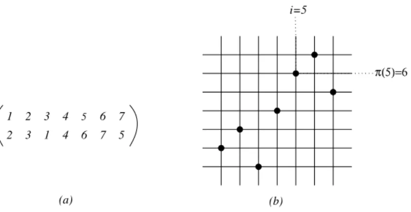
A permutation � of length � can be represented in three diferent ways: 1. Two-lines notation: this is perhaps the most widely used method to

represent a permutation and consists in organizing in the top row the numbers from 1 to � in ascending order and their image in the bottom row, as shown in Figure 1.7 (�).

2. One-line notation: in this case only the second row of the corresponding two-lines notation is used.

3. Graphical representation: it corresponds to the graph �(�) =_{{(�, �}i) : 1≤ � ≤ �} ⊆ [1, �] × [1, �] . An example of �(�) is displayed in Figure 1.7 (�).

(24)

1 2 3 4 5 6 7 2 3 1 4 6 7 5 (a) i=5 π(5)=6 (b)

Figure 1.7: Two-lines representation of the permutation � = 2314675 in (�) and in (�) the graphical representation of �.

Let � be a permutation; � is a ixed point of � if �i = �and an exceedance of � if �i > �. The number of ixed points and exceedances of � are indicated with ��(�) and ��(�) respectively.

An element of a permutation that is neither a ixed point nor an ex-ceedance, i.e. an � for which �i < �, is called deiciency. Permutations with no ixed points are often referred to as derangements.

We say that � ≤ � − 1 is a descent of � ∈ Sn if �i > �i+1. Similarly, � _{≤ � − 1 is an ascent of � ∈ S}n if �i < �i+1. The number of descents and ascents of � are indicated with ��(�) and ��(�) respectively.

Given a permutation �, we can deine the following subsets of points [22]: 1. the set of right-to-left minima as the set of points:

{(�, �i) : �i < �j ∀�, 1 ≤ � < �} ; 2. the set of right-to-left maxima as the set of points:

{(�, �i) : �i > �j ∀�, 1 ≤ � < �} ; 3. the set of left-to-right minima as the set of points:

{(�, �i) : �i < �j ∀�, � < � ≤ �} ; 4. the set of left-to-right maxima as the set of points:

(25)

(a) (b) (c) (d)

Figure 1.8: (�) Set of to-left minima for � = 21546837; (�) set of right-to-left maxima; (�) set of left-to-right minima; and (�) set of left-to-right maxima.

An example of each of the sets deined above is provided in Figure 1.8. Let ��(�) denote the length of the longest increasing subsequence of �, i.e., the largest � for which there exist indexes �1 < �2 <· · · < �m such that �i1 < �i2 <· · · < �im.

Deine the rank of �, denoted ��(�), to be the largest � such that �i > � for all � ≤ �. For example, if � = 63528174, then ��(�) = 1, ��(�) = 4, ��(�) = 4 and ��(�) = 2.

We say that a permutation � ∈ Sn is an involution if � = �−1. The set of involutions of length � is indicated with In.

1.3.2 Pattern avoiding permutations

The concept of permutation patterns proved useful in many branches of Mathematics literature, as supported by the several works produced in the last decades. A comprehensive overview, “Patterns in Permutations”, has been proposed by Kitaev in [92].

Deinition 10. Let �, � be two positive integers with � ≤ �, and let � ∈ Sn and � ∈ Sm be two permutations. We say that � contains � if there exist indexes �1 < �2 < · · · < �m such that �i1�i2· · · �im is in the same relative order as �1�2· · · �m (that is, for all indexes � and �, �ia < �ib if and only if �a < �b). In that case, �i1�i2· · · �im is called an occurrence of � in � and we write � 4S �. In this context, � is also called a pattern.

If � does not contain �, we say that � avoids �, or that � is �-avoiding. For example, if � = 231, then � = 24531 contains 231, because the subsequence �2�3�5 = 451 has the same relative order as 231. However, � = 51423 is

(26)

231-avoiding. We indicate with ��n(�) the set of �-avoiding permutations in Sn.

Deinition 11. A permutation class is a set of permutations C that is down-ward closed for 4S: for all � ∈ C, if � 4S �, then � ∈ C.

In other terms, a family of permutations is a permutation class if it is an order ideal of the poset (S, 4S). We remark that a permutation class is also known as a closed class, or pattern class, or simply class of permutations, see for example in [1, 4].

It is a natural generalisation to consider permutations that avoid several patterns at the same time. If B ⊆ Sk, � ≥ 1, is any inite set of patterns, we denote by ��n(B), also called B-avoiding permutation, the set of permu-tations in Sn that avoid simultaneously all the patterns in B. For example, if B = {123, 231}, then ��4(B) = {1432, 2143, 3214, 4132, 4213, 4312, 4321}. We remark that for every set B, ��n(B) is a permutation class.

The sets of permutations pairwise-uncomparable with respect to the order relation (4S) are called antichains.

Deinition 12. If B is an antichain, then B is unique and is called basis of the permutation class ��n(B). In this case, it also true that

B=_{{� /}_{∈ ��}n(B) : ∀� 4S �, � ∈ ��n(B)} .

Proposition 13. Let be C = ��n(B1) = ��n(B2). If B1 and B2 are two antichains then B1 = B2.

Proposition 14. A permutation class C is a family of pattern-avoiding per-mutations and so it is characterised by its basis.

One can ind more details and in particular the proofs of the previous propositions in [22].

Even though the majority of permutation classes analysed in literature are characterised by inite bases, there exist permutation classes with ininite basis (e.g. the pin permutations in [30]). Deciding whether a certain per-mutation class is characterised by a inite or ininite basis is not an entirely solved problem; some hints on the decision criteria can be found in [1, 5]. Results on pattern avoidance

Deinition 15. Two patterns are Wilf equivalent and belong to the same Wilf class if, for each �, the same number of permutations of length � avoids the same pattern.

(27)

Wilf equivalence is a very important topic in the study of patterns. The smallest example of non-trivial Wilf equivalence is for the classical patterns of length 3; all six patterns 123, 321, 132, 213, 231, and 312 are Wilf equiv-alent; each pattern is avoided by �n permutations of length �, where �n is the Catalan number 1

n+1 ︀_2n

n ︀

, see for example [108, 113, 123].

By extension, we can deine the strongly Wilf equivalence as follows. Deinition 16. Two patterns � and � are strongly Wilf equivalent if they have the same distribution on the set of permutations of length � for each �, that is, if for each nonnegative integer � the number of permutations of length � with exactly � occurrences of � is the same as that for �.

For example, � = 132 is strongly Wilf equivalent to � = 231, since the bijection deined by reversing a permutation turns an occurrence of � into an occurrence of � and conversely. On the other hand, 132 and 123 are not strongly Wilf equivalent, although they are Wilf equivalent. Furthermore, the permutation 1234 has four occurrences of 123, but there is no permutation of length 4 with four occurrences of 132.

A thoroughly investigated problem is the enumeration of elements in a given permutation class C for any integer �. Recent results in this direction can be found in [83, 92] (respectively, 1995 and 2003). However, such an enumeration problem was already known since 1973 thanks to the work of Knuth [98], where permutations avoiding the pattern 231 were considered.

As for the case of patterns of length three, for length four we can reduce the problem by considering the seven symmetrical classes in order to obtain the sequences of enumeration. Some results relatively to these patterns ap-pear in [22]. Only the problem of enumerating permutations avoiding 4231 (or 1324) remains unsolved.

In 1990, Stanley and Wilf conjectured that, for all classes C, there exists a constant � such that for all integers � the number of elements in Cn = C∩ Sn is less than or equal to �n_{. In 2004, Marcus and Tardos [101] proved the} Stanley-Wilf conjecture. Before that result, Arratia [3] showed that, being C_n= ��n(�), the conjecture was equivalent to the existence of the limit:

�� (�) = lim

n→∞��n(�) , which is called the Stanley-Wilf limit for �.

The Stanley-Wilf limit is 4 for all patterns of length three, which follows from the fact that the number of avoiders of any one of these is the �th Catalan number �n, as mentioned above. This limit is known to be 8 for the pattern 1342 (see [23]). For the pattern 1234, the limit is 9; such limit

(28)

was obtained as a special case of a result of Regev [107, 106], who provided a formula for the asymptotic growth of the number of standard Young tableaux with at most � rows. The same limit can also be derived from Gessel’s general result [77] for the number of avoiders of an increasing pattern of any length. The only Wilf class of patterns of length four for which the Stanley-Wilf limit is unknown is represented by 1324, although a lower bound of 9.47 was established by Albert et al. [2]. Later, Bóna [21] was able to reine this bound by resorting to the method in [47]; inally, Madras and Liu [100] estimated that the limit for the pattern1324 lies, with high likelihood, in the interval [10.71, 11.83]4.

Finally, considering a permutation as a bijection we can look at notions such as ixed points and exceedances. This new way to see a permutation makes relevant the study of statistics together with the notion of pattern avoidance. There is a lot of literature devoted to permutation statistics (see for example [63, 72, 75, 78]).

1.3.3 Generalised patterns and other new patterns

Babson and Steingrímsson [7] introduced the notion of generalised patterns, which requires that two adjacent letters in a pattern must be adjacent in the permutation, as shown in Figure 1.9 (�). The authors introduced such patterns to classify the family of Mahonian permutation statistics, which are uniformly distributed according to the number of inversions.

(a) (b) (c) (d)

Figure 1.9: (�) Classical pattern 3 − 1 − 4 − 2; (�) Generalised (or vincular) pattern 3 − 1 − 42: (�) Bivincular pattern (3142, {1}, {3}); and (�) Mesh pattern (3142, �).

A generalised pattern is written as a sequence wherein two adjacent el-ements may or may not be separated by a dash. With this notation, we indicate a classical pattern with dashes between any two adjacent letters of

4_{This result was obtained by using Markov chain Monte Carlo methods to generate}

(29)

the pattern (for example, 1423 as 1 − 4 − 2 − 3). If we omit the dash be-tween two letters, we mean that the corresponding elements of � have to be adjacent. For example, in an occurrence of the pattern 12 − 3 − 4 in a permutation �, the entries in � that correspond to 1 and 2 are adjacent. The permutation � = 3542617 has only one occurrence of the pattern 12 − 3 − 4, namely the subsequence 3567, whereas � has two occurrences of the pattern 1_{− 2 − 3 − 4, namely the subsequences 3567 and 3467.}

If � is a generalised pattern, ��n(�)denotes the set of permutations in Sn that have no occurrences of � in the sense described above. Throughout this chapter, a pattern represented with no dashes will always denote a classical pattern, i.e. one with no requirement about elements being consecutive, unless otherwise speciied.

Several enumerative results on permutations classes avoiding generalised patterns have been achieved. Claesson obtained the enumeration of permuta-tions avoiding a generalised pattern of length three [46] and of permutapermuta-tions avoiding two generalised patterns of length three [48]. Another result in terms of permutations avoiding a set of generalised patterns of length three was obtained by Bernini et al. in [17, 18], where the enumeration of permu-tations avoiding sets of generalised patterns as a function of its length and another parameter.

Another kind of patterns, called bivincular patterns, was introduced by Bousquet-Mélou et al. in [26] with the aim to increase the symmetries of the classical patterns. A bijection between permutations avoiding a particular bivincular pattern was derived, as well as several other families of combina-torial objects.

Deinition 17. Let � = (�, �, � ) be a triple where � is a permutation of Sn and � and � are subsets of {0} ∪ [�]. An occurrence of � in � is a subsequence � = (�i1,· · · , �ik)such that � is an occurrence of � in � and, with (�1 < �2 < · · · < �k) being the set {�i1,· · · , �ik} ordered (so �1 = ��m�im etc.), and �0 = �0 = 0 and �k+1 = �k+1 = � + 1,

�x+1 = �x+ 1 ∀� ∈ � and �y+1 = �y + 1 ∀� ∈ � .

Bivincular patterns are graphically represented by graying out the corre-sponding columns and rows in the Cartesian plane as shown in Figure 1.9 (�). Clearly, bivincular patterns (�, ∅, ∅) coincide with the classical patterns, while bivincular patterns (�, �, ∅) coincide with the generalised patterns (hence, we refer to them as vincular in the sequel).

We now give the deinition of Mesh patterns, which were introduced in [34] to generalise multiple varieties of permutation patterns. To do so, we

(30)

extend the above prohibitions determined by grayed out columns and rows to graying out an arbitrary subset of squares in the diagram.

Deinition 18. A mesh pattern is an ordered pair (�, �), where � is a permu-tation of Skand � is a subset of the (�+1)2 unit squares in [0, �+1]×[0, �+1], indexed by they lower-left corners.

Thus, in an occurrence of (3142, �) in a permutation �, where � = {(0, 2), (1, 4), (4, 2)}) in Figure 1.9 (�), for example, there cannot be a letter in � that precedes all letters in the occurrence and lies between the values of those corresponding to the 1 and the 3. This is illustrated by the shaded square in the leftmost column. For example, in the permutation 425163, 5163 is not an occurrence of (3142, �), since 4 precedes 5 and lies between 5 and 1 in value, whereas the subsequence 4263 is an occurrence of this mesh pattern.

The reader may ind an extension of mesh patterns in [121], where are characterised all mesh patterns in which the mesh is superluous.

The results on Wilf equivalent classes have then been extended to bivincu-lar patterns and mesh patterns. For example there is in [104] the classiication of all bivincular patterns of length two and three according to the number of permutations avoiding them, and a partial classiication of mesh patterns of small length in [86].

1.4 Partially ordered sets

In this section we recall the basic notions and the most important deinitions on partially ordered sets (posets). For a more in-depth presentation, the interested reader may consult [115].

Deinition 19. A partially ordered set or poset is a pair � = (�; ≤) where � is a set and ≤ is a relexive, antisymmetric, and transitive binary relation on �.

� is referred to as the ground set, while ≤ � is a partial order on �. Elements of the ground set � are also called points. A poset is inite if the ground set is inite.

In our work, we consider only inite posets. Of course, the notation � < � in � means � ≤ � in � and � ̸= �. When a poset does not change throughout some analysis, we ind convenient to abbreviate � ≤ � in � with � ≤P �. If �, � _{∈ � and either � ≤ � or � ≤ �, we say that � and � are comparable in} �; otherwise, we say that � and � are uncomparable in � .

(31)

Deinition 20. A partial order � = (�; ≤) is called total order (or linear order) if for all �, � ∈ �, either � ≤ � in � or � ≤ � in � .

Deinition 21. Let �, � be two generic elements in �. A partial order � = (�;≤) is called lattice when there exist two elements, usually denoted by �∨� and by � ∧ �, such that:

❼ � ∨ � is the supremum of the set {�, �} in � ❼ � ∧ � is the inimum of the set {�, �} in � , i.e. for all � in �

� ≥ � ∨ � ⇐⇒ � ≥ � and � ≥ � � _{≤ � ∧ � ⇐⇒ � ≤ � and � ≤ � .}

Deinition 22. Given �, � in a poset � , the interval [�, �] is the poset {� ∈ � : �≤ � ≤ �} with the same order as � .

Deinition 23. Let � = (�, ≤) be a poset and let � and � be distinct points of �. We say that “� is covered by �” in � when � < � in � , and there is no point � ∈ � for which � < � in � and � < � in � .

In some cases, it may be convenient to represent a poset with a diagram of the cover graph in the Euclidean plane. To do so, we choose a standard horizontal/vertical coordinate system in the plane and require that the ver-tical coordinate of the point corresponding to � be larger than the verver-tical coordinate of the point corresponding to � whenever � covers � in � . Each edge in the cover graph is represented by a straight line segment which con-tains no point corresponding to any element in the poset other than those associated with its two endpoints. Such diagrams, called Hasse diagrams, are deined as follows.

Deinition 24. The Hasse diagram of a partially ordered set � is the (di-rected) graph whose vertices are the elements of � and whose edges are the pairs (�, �) for which � covers �. It is usually drawn so that elements are placed higher than the elements they cover.

The Boolean algebra �n is the set of subsets of [�], ordered by inclusion (� ≤ � means � ⊆ � ). Generalising �n, any collection � of subsets of a ixed set � is a partially ordered set ordered by inclusion. Figure 1.10 displays the diagram obtained with � = 3.

In particular, Hasse diagrams are useful to visualize various properties of posets.

(32)

{O} {1,2,3} {1,3} {2,3} {3} {2} {1} {1,2}

Figure 1.10: The Hasse diagram of �3.

Deinition 25. A linear extension of a poset � = (�, ≤), where � has cardinality |�|, is a bijection � : � → {1, 2, · · · , |�|} such that � < � in � implies �(�) < �(�).

Deinition 26. If � = (�, ≤) is a poset and � ⊆ �, then

�P(� ) = {� ∈ � : ∀� ∈ �, � > �} and �P(� ) = {� ∈ � : ∀� ∈ �, � < �} are called respectively the ilter and the ideal of � generated by � .

An ideal or ilter is principal when it is generated by a singleton. Then D_P =_{�P({�}) : � ∈ �} and UP ={�P({�}) : � ∈ �} are respectively the set of principal ideals of � and the set of principal ilters of � .

An equivalence relation ≡ on X is built as follows:

�_{≡ � ⇐⇒ �� ({�}) = �� ({�}) and �}P({�}) = �P({�}) .

1.4.1 Operations on partially ordered sets

Given two partially ordered sets � and �, we deine the following new par-tially ordered sets:

1. Disjoint union. � +� is the disjoint union set � ∪�, where � ≤P+Q� if and only if one of the following conditions holds:

❼ �, � ∈ � and � ≤P � ❼ �, � ∈ � and � ≤Q �

(33)

The Hasse diagram of � + � consists of the Hasse diagrams of � and � drawn together.

2. Ordinal sum. � ⊕ � is the set � ∪ �, where � ≤P ⊕Q� if and only if one of the following conditions holds:

❼ � ≤P+Q �

❼ � ∈ � and � ∈ �

Note that the ordinal sum operation is not commutative: in � ⊕ �, everything in � is less than everything in �.

The posets that can be described by using the operations ⊕ and + starting from the single element poset (usually denoted by 1) are called series parallel orders [115]. This set of posets has a nice characterisation in terms of subposet avoiding.

3. Cartesian product. � × � is the Cartesian product set {(�, �) : � ∈ �, � ∈ �}, where (�, �) ≤P ×Q (�′, �′) if and only if both � ≤P �′ and �_≤Q �′. The Hasse diagram of � × � is the Cartesian product of the Hasse diagrams of � and �.

Deinition 27. A chain of a partially ordered set � is a totally ordered subset � _{⊆ � , with � = {�}0,· · · , �} with �0 ≤ · · · ≤ �l. The quantity � = |�| − 1 is the length of the chain and is equal to the number of edges in its Hasse diagram.

If 1 denotes the single element poset, then a chain composed by � elements is the poset obtained by performing the ordinal sum exactly � times:

1⊕ 1 ⊕ · · · ⊕ 1 .

Deinition 28. A chain is maximal if there exist no other chain strictly containing it.

Deinition 29. The rank of � is the length of the longest chain in � . The set of all permutations forms a poset � with respect to classical pattern containment. That is, a permutation � is smaller than � (written � 4S �) if � occurs as a pattern in �. This poset is the underlying object of all studies on pattern avoidance and containment.

(34)

Chapter 2 �

-parallelogram polyominoes:

characterisation and enumeration

In this chapter we consider the problem of enumerating a subfamily of �-convex polyominoes. We recall (see Section 1.1 for more details) that a convex polyomino is �-convex if every pair of its cells can be connected by means of a monotone path, internal to the polyomino (see Figure 2.1 (�) and (�)), and having at most � direction changes. In the literature we ind some results regarding the enumeration of �-convex polyominoes of given semi-perimeter, but only for small values of �, precisely � = 1, 2, see again Chapter 1 for more details.

As counting �-convex polyominoes seems diicult, we tackle the problem of counting the set Pk of �-parallelogram ones. Figure 2.1 (�) shows an example of convex polyomino that is not parallelogram, while Figure 2.1 (�) depicts a 4-parallelogram (non 3-parallelogram) polyomino.

(a) (b) (c)

Figure 2.1: (�) A convex polyomino; (�) a monotone path between two cells of the polyomino with four direction changes; (�) a 4-parallelogram.

The family Pkof �-parallelogram polyominoes can be treated in a simpler way than �-convex polyominoes, since we can use the fact that a

(35)

parallelo-gram polyomino is �-convex if and only if there exists at least one monotone path having at most � direction changes running from the lower leftmost cell to the upper rightmost cell of the polyomino. Indeed, this property is used to partition the family Pk into three subfamilies, namely the lat, right, and up �-parallelogram polyominoes, and we will provide an unambiguous decom-position for each of them. Doing so we obtain the generating functions of the three families and then of �-parallelogram polyominoes. An interesting fact is that, while the generating function of parallelogram polyominoes is al-gebraic, for every � the generating function of �-parallelogram polyominoes is rational. Moreover, we are able to express such generating function as continued fractions, and then in terms of the known Fibonacci polynomials. Since we are able to express the generating function of Pk in terms of Fi-bonacci polynomials, we have been able to ind a simpler proof, using rooted plane trees. More precisely, in [53] it is proved that the generating function of plane trees having height less than or equal to a ixed value can be expressed using Fibonacci polynomials and so we found a bijection between these two objects. Some of the topics of this chapter have been treated in [12].

To our opinion, this work is a irst step towards the enumeration of �-convex polyominoes, since it is possible to apply our decomposition strategy to some larger families of �-convex polyominoes (such as, for instance, di-rected �-convex polyominoes).

2.1 Classiication and decomposition of P

�

Let us start by ixing some terminology which is useful in the rest of the section.

Following Deinition 5 in Section 1.1 we can represent an internal path as a sequence of cells.

Deinition 30. Let be � and �′ two distinct cells of a polyomino; an internal path from � to �′_{, denoted �}

AA′, is a sequence of distinct cells (�₁,· · · , �_n) such that �1 = �, �n = �′ and every two consecutive cells in this sequence are edge-connected.

Henceforth, since polyominoes are deined up to translation, we assume that the center of each cell of a polyomino corresponds to a point of the plane Z× Z, and that the center of the lower leftmost cell of the minimal bounding rectangle (denoted by m.b.r.) of a polyomino corresponds to the origin of the axes. In our case, since we work with parallelogram polyominoes, the lower leftmost cell of the m.b.r belongs to the polyomino. So, according to the

(36)

respective position of the cells �i and �i+1, we say that the pair (�i, �i+1) forms:

1. a north step � in the path if (�i+1, �i+1) = (�i, �i+ 1); 2. an east step � in the path if (�i+1, �i+1) = (�i+ 1, �i); 3. a west step � in the path if (�i+1, �i+1) = (�i− 1, �i); 4. a south step � in the path if (�i+1, �i+1) = (�i, �i− 1).

Moreover, since our polyominoes are also convex, for obvious reasons of sym-metry, we will deal only with monotone paths using steps � or �.

Deinition 31. Let � be a parallelogram polyomino and � an internal path. We call side every maximal sequence of steps of the same type into �. Remark 32. Let � be a parallelogram polyomino. We denote by � and � the lower leftmost cell and the upper rightmost cell of � , respectively.

Deinition 33. The vertical (horizontal) path �(� ) (respectively ℎ(� )) is an internal path -if it exists- running from � to �, and starting with a step � (respectively �), where every side has maximal length (see Figure 2.3).

From now on, in the graphical representation, the path will be represented using lines rather than cells. In practice, to represent the path we use a line joining the centers of the cells, more precisely a dashed line to represent �(� ) and a solid one for ℎ(� ). Observe that our deinition does not work if the irst column (resp. row) of � is made of one cell, and in this case by convention �(� ) and ℎ(� ) coincide (Figure 2.3 (�)). Henceforth, if there are no ambiguity we write � (resp. ℎ) in place of �(� ) (resp. ℎ(� )). So, by deinition, a cell �i of � (or �i of ℎ) could correspond to one of two possible types of direction changes, more precisely

- to a change e-n if (�Vi+ 1, �Vi) /∈ � (resp. (�Hi + 1, �Hi) /∈ � ); - to a change n-e if (�Vi, �Vi + 1) /∈ � (resp. (�Hi, �Hi+ 1) /∈ � ).

These two paths distinguish two types of cells into the polyomino at every direction change. So, considering ℎ(� ) = (�1 = �,· · · , �n = �) (respectively �(� ) = (�1 = �,· · · , �n= �)), we can characterise each cell of � that is not in ℎ(� ) (or �(� )) as follows: for every cell � ∈ � , � /∈ ℎ(� ) (resp. � /∈ �(� )), there exists an index �, 1 < � ≤ �, such that

(37)

(resp. �B > �Vi and �B = �Vi or �B < �Vi and �B = �Vi). We say that in the irst case � is a cell of type left-top, and in the second case that � is a cell of type right-bottom. The reader can observe in Figure 2.2 that the cell � is an example of cell right-bottom, in fact �B < �V4 and �B = �V4 and that �′ is an example of cell left-top, in fact �B′ > �V8 and �B′ = �_V8. V8 V4 E S B’ B

Figure 2.2: An example of 4-parallelogram polyomino and the internal path � = (�1 = �, �2,· · · , �20 = �).

Now, we are ready to prove the following important property.

Proposition 34. The convexity degree of a parallelogram polyomino � is equal to the minimal number of direction changes required to any path running from � to �.

Proof. Let � be a polyomino and let be � the minimal number of direction changes among ℎ and �. We want to prove that for every two cells of � , � and �′ _{diferent from � and �, exists a path �}

AA′ having at most � direction changes. We have to take into consideration three diferent cases.

1. Both � and �′ _{belong to � (or ℎ).}

This case is trivial because the path running from � to �′_{, �}

AA′, is a subpath of � (or ℎ), so the number of direction changes is less than or equal to �.

2. Only one between � and �′ _{belongs to � (or ℎ).}

(38)

to � (or ℎ) and that � is a cell of type left-top. Then, there exists an index � such that �A> �Vi and �A = �Vi (or �A < �Hi and �A= �Hi), so with �Vi − �A (or �Hi − �A) steps � (or �) we can reach the path � (or ℎ) with only one direction change but after � (or ℎ) have changed its direction at least once. At this point it is easy to see that the path �AA′ has at most � direction changes, the irst to reach the path � (or ℎ) and the subsequent ones are those made by the subpath of � (or of ℎ) to reach the cell �′.

3. Neither � nor �′ _{belong to � (or ℎ).}

The proof is similar to that one of the previous case.

Proposition 35. The number of direction changes that ℎ and � require to run from � to � may difer at most by one.

The proof is similar to the proof above and it is left to the reader. Also the following property is straightforward.

Proposition 36. A polyomino � is �-parallelogram if and only if at least one among �(� ) and ℎ(� ) has at most � direction changes.

We begin our study with the family Pk of �-parallelogram polyominoes where the convexity degree is exactly equal to � ≥ 0. Then the enumeration of Pk will readily follow, in fact Pk = ∪ki=1Pi. According to our deinition, P0 is made of horizontal and vertical bars of any length.

In any given parallelogram polyomino � , let �(� ) (briely, �) be the earliest point in the two paths ℎ and � such that the tails coincide (see Figure 2.3 (�), (�)). Clearly � may even coincide with � (see Figure 2.3 (�)) or with �. Figure 2.3 depicts the various positions of � into a parallelogram polyomino.

From now on, unless otherwise speciied, we always assume that � ≥ 1. Let us give a classiication of the polyominoes in Pk, based on the position of the cell � inside the polyomino.

Deinition 37. A polyomino � in Pk is said to be

1. a lat �-parallelogram polyomino if � coincides with �. The family of these polyominoes is denoted by Pk;

2. an up (resp. right) �-parallelogram polyomino, if � is distinct from � and ℎ and � end with a step � (resp. �). The family of up (resp. right) �-parallelogram polyominoes is denoted by PU