HAL Id: halshs-00185370
https://halshs.archives-ouvertes.fr/halshs-00185370
Submitted on 5 Nov 2007
HAL is a multi-disciplinary open access
archive for the deposit and dissemination of sci-entific research documents, whether they are pub-lished or not. The documents may come from
L’archive ouverte pluridisciplinaire HAL, est destinée au dépôt et à la diffusion de documents scientifiques de niveau recherche, publiés ou non, émanant des établissements d’enseignement et de
Fractional seasonality: Models and Application to
Economic Activity in the Euro Area
Laurent Ferrara, Dominique Guegan
To cite this version:
Laurent Ferrara, Dominique Guegan. Fractional seasonality: Models and Application to Economic Activity in the Euro Area. Conference on Seasonality, Seasonal Adjustment and their Implications for Short-Term Analysis and Forecasting, May 2006, Luxembourg. pp.137 - 153. �halshs-00185370�
Fractional seasonality: Models and
Application to Economic Activity in the
Euro Area
∗
L. Ferrara
†and D. Guégan
‡June 2006
Abstract:
Many time series reflecting the economic activity are affected by a strong seasonal behavior as well as by long-range dependence characterized, in the spectral domain, by peaks at the seasonal frequencies. In recent years, frac-tionally integrated seasonal models have been proposed in the statistical liter-ature to take those stylized facts into account, see for instance Porter-Hudak (1990) or Hassler (1994). Generalized long memory models introduced by Gray, Zhang and Woodward (1989, 1994), based on Gegenbauer polynomi-als, have been proved to be an attractive alternative to such models when dealing with real data (see Ferrara and Guégan, 2001a, 2001b). In this paper, we recall some concepts on seasonal long memory, we review the diverse frac-tionally integrated seasonal time series models and we discuss their statistical properties. Then, we compare the empirical performances of those models on euro area economic data and we show that generalized long memory models offer competitive alternatives to classical SARIMA models, avoiding over-differentiation and providing a better goodness of fit.
Keywords:
Fractional seasonality, long-range dependence, generalized long memory mod-els, economic activity.
∗Paper presented at the Conference for Seasonality, Seasonal Adjustement and their
Implications for Short-Term Analysis and Forecasting, organized by Eurostat, Luxem-bourg, May 2006. We thank the organizers for the invitation.
†Centre d’Observation Economique de la Chambre de Commerce et d’Industrie de Paris
and Centre d’Economie de la Sorbonne - Antenne Cachan, Département d’Economie et Gestion de l’ENS Cachan, e-mail : ferrara@ces.ens-cachan.fr
‡Centre d’Economie de la Sorbonne - Antenne Cachan, Département d’Economie et
1
Introduction
Many economic time series display seasonal fluctuations inherent to the eco-nomic activity. Therefore, models allowing to describe the seasonal compo-nents of the data are essential to accurately analyse and forecast business quantities.
During a long time, in economic time series, the seasonal and / or cyclical movements have been modelled using non-stationary short memory processes, like the classical SARIMA model, which includes seasonal unit roots in its expression. Those models have the specificity to exhibit peaks at seasonal fre-quencies in the spectral density. Now, several kinds of non-seasonal processes with a cyclical movement have been proposed in the literature. They simi-larly produce peaks in the spectral density at frequencies but no necessarily equal to the seasonal ones.
A first generation of those processes referred to as fractionally differenced ARMA models has been developed to take into account infinite cycle. Thus, the first fractional model (FARMA) introduced by Granger and Joyeux (1980) and Hosking (1981) uses a differencing operator of the form (I − B)d, where
d is allowed to take non-integer values. When the fractional differencing parameter d is greater than zero, the process exhibits long memory in the sense that observations, a long time-span apart, have non-negligible depen-dence. The process is also referred to as strongly dependent, see Guégan and Ladoucette (2001) for further details. This is in contrast to a weakly dependent or a strong mixing process, in which the maximal dependence between two observations becomes almost non-existent as the time span be-tween them increases. Thus, FARMA models are useful for describing data which have both short-term correlation (ARMA component) and correlation between observations a long time-span apart (fractional component). The FARMA models are characterized by a slow decay of the auto-correlation function (ACF) at an hyperbolic rate. In the spectral domain, FARMA processes present a peak for very low frequencies, close to the zero frequency. However, those models do not permit to take presence of seasonality inside the data into account.
Thus, a second generation of models dedicated to take seasonal or cycli-cal components with persistence has been developed. Those models include generalized long memory processes and seasonal long memory processes (see the review in the next section). Such kinds of models are well appropriate for data with short term-dependent (seasonal or non-seasonal) ARMA
com-ponents and slowly decaying auto-correlation at periodic lags. The use of fractional seasonal degrees allows to take seasonal fluctuations into account while avoiding over-differentiation. The ACF of a seasonal fractionally in-tegrated model displays an hyperbolic decay at seasonal lags, rather than the slow linear decay characterizing the conventional seasonal differencing model. Indeed, we generally observe on the ACF of real data a superposition of hyperbolically damped sin waves.
In the spectral domain, a peak in the spectral density at a given frequency λ indicates a cycle of period 2π
λ in the process. More general cases arise with
the presence of several peaks in the spectral density located at the seasonal frequencies λh = 2πhs , h = 1, . . . , [s/2], where s is the number of observations
per year (s = 1 for annual data, s = 4 for quarterly data, s = 12 for monthly data and s = 52 for weekly data), and [s/2] denotes the integer part of s/2. Then a process (Xt)t with such a spectral density is referred to as a seasonal
process.
In this paper, we are interested in reviewing some models allowing to de-scribe jointly these phenomena and we apply them to real data of economic activity in the euro area. As regards applications to real data, the simul-taneous presence of long memory and seasonality in business and economic data has received some attention in the literature. For instance, Carlin and Dempster (1989) consider monthly unemployment rate of US males; Porter Hudak (1990) deals with the US money supply and monetary aggregates and Ray (1993) proposes models for monthly IBM revenue data. Monthly UK in-flation rates have been considered by Franses and Ooms (1997), Arteche and Robinson (2000) and Arteche (2003). Other applications deal with time series on food and tobacco and non-durable consumer goods (Darné, Guiraud and Terraza, 2004), public transportation (Ferrara and Guégan, 2000), exchange rates (Ferrara and Guégan, 2001a) and spot prices (Ferrara and Guégan, 2001b), German electricity prices (Diongue and Guégan, 2004). For all those applications, a specific model has been proposed. Generally the choice of the model correspond to a specific problematic and in most cases no comparison has been done with different seasonal long memory models. In this paper, our approach is slighty different insofar as we compare competitive models for the same data set.
The plan of the paper is the following: in section two we review the dif-ferent models taking long memory ans seasonality into account. Section three presents two applications showing that the generalized long memory approach through Gegenbauer filters appears to be a very interesting tool in
some cases. Last, section four concludes.
2
The models: A review
This section describes commonly used parametric models inside the class of stochastic seasonal processes whose spectral density has a singularity or a zero at any frequency ω, 0 < ω ≤ π, such that:
f (ω + λ) ∼ C|λ|−2d, as, λ → 0, |d| < 1/2, (1)
where C is a positive constant. Thus f (λ) has a pole at λ = ω if d > 0 and a zero if d < 0. When f (λ) satisfies the equation (1) for every seasonal frequency ω = ωh, h = 1, 2, · · · , [s/2], possibly with the memory parameter,
d, varying across h, we say that the process has a seasonal long memory behavior. However, for non seasonal time series, like annual data, equation (1) holds for a single ω ∈ (0, π] as well as ω = 0.
Processes with a seasonal long memory behavior can also be described in terms of their autocovariances function γ. A characteristic of autocovariances of such processes is the oscillating slow decay such that often γh = O(h2d−1),
as h → ∞, but with oscillations whose amplitude depends on ω instead of the eventual monotonic decay describes like γh ∼ Kh2d−1, as h → ∞, for
standard long memory processes at frequency zero.
The models traditionally used for seasonal and cyclical time series are either stationary short memory processes or non-stationary processes, due to a de-terministic component (seasonal dummies) or to a stochastic trend (seasonal unit roots). We do not consider this approach in this section.
In order to allow for different persistence parameters across different frequen-cies, we can consider the following general representation for a seasonal long memory process. We will see how it nests all the particular models intro-duced from the nineties in the literature to take both the seasonal and /or cyclical behaviors and the long memory component of the data into account.
Without loss of generality, we assume that (Xt)t is a zero mean process
and for the moment we assume that (Xt)t is a stationary process. The
Seasonal/Cyclical Long Memory (SCLM) filter is defined as follows:
F (B) = (I − B)d0
k−1
Y
i=1
B is the backshift operator, for i = 1, · · · , k − 1, λi can be any frequency
between 0 and π and di ∈ R. Now we can apply the filter F (B) described in
(2) to the process (Xt)t to take into account its main characteristics, thus:
(I − B)d0
k−1
Y
i=1
(I − 2Bcosλi+ B2)di(I + B)dkXt = εt, (3)
where (εt)t has continuous and positive spectrum. We say that the process
(Xt)t is integrated of order di at frequency λi, Iλi(di), for i = 0, 1, 2, · · · , k
where λ0 = 0 and λh = π.
This model has been first discussed by Robinson (1994) in order to test whether the data stem from a stationary or a non-stationary process. In that latter case the representation of the model is the following:
(I − B)d0+θ0 k−1 Y i=1 (I − 2Bcosλi+ B 2 )di+θi(I + B)dk+θkX t= εt, (4)
where for i = 0, 1, · · · k, θi ∈ [−1, 1] and |di| < 1/2. Robinson tests the null of
the parameter θi, i = 0, 1, · · · k. Gil-Alana (2001) and Arteche (2003) test for
the model (3), the constancy of the parameters across the different frequen-cies. Chan and Palma (2005) study the asymptotic behavior of the estimated parameters of model (3) using the pseudo-maximum likelihood method.
Remark that this general representation (3) nests a lot of seasonal or cyclical fractional models introduced in the literature and which can be competitive in order to take those specific behaviors into account. Below, we specify those models.
• If (εt)t is a stationary invertible ARMA(p,q) process, Giraitis and
Lei-pus (1995) used the terminology ARUMA for such process (Xt)t
verify-ing the equation (3) when |di| < 1/2, for i = 0, 1, · · · , h. In that latter
case the filter F (B) is equal to F (B) = 1 − u1B − · · · , −udBd and it
has a finite number of zeros or singularities of order di, (|di| < 1/2) on
the unit circle allowing to model seasonal periodicities. Parameter es-timation has been considered by Anderson (1979) and Huang and Anh (1993). This model is not very useful in practice in terms of a modelling strategy, thus the following model (5) appears more interesting. • A simple case of the model (3), assuming d0 = 0 gives the classical
k-factor Gegenbauer process whose representation is given by:
k
Y
i=1
with, for i = 1, . . . , k, νi = cos(λi), the frequencies λi = cos−1(νi)
being the Gegenbauer frequencies or the G-frequencies. This model, introduced by Giraitis and Leipus (1995), see also Woodward, Cheng and Gray (1998) takes different kinds of waves in the ACF and describes jointly k persistent periodicities in the data. With this model we do not consider the existence of an infinite cycle. In the presence of a short memory component, the model (5), assuming |di| < 1/2, i = 1, · · · , k,
is referred to as a k-factor GARMA process and Giraitis and Leipus (1995) estimate the parameters of this model using a Whittle estimation procedure. Its spectral density is given by :
fX(λ) = σ2 ε 2π |θ(eiλ)|2 |φ(eiλ)|2 k Y i=1 |2(cos(λ) − νi)|−2di (6) = σ 2 ε 2π |θ(eiλ)|2 |φ(eiλ)|2 k Y i=1 4 sin(λ + λi 2 ) sin( λ − λi 2 ) −2di , (7)
where 0 ≤ λ ≤ π and for i = 1, . . . , k, the frequencies λi = cos−1(νi) are
the G-frequencies, and φ(.) and θ(.) are respectively the autoregressive and moving-average polynomials of the short memory part.
• When k = 1 in (5), we get, under the same assumptions as before, the GARMA model, introduced by Gray, Zhang and Woodward (1989) whose representation (without short memory terms) is:
(I − 2 cos λB + B2
)dXt = εt, (8)
where (εt)t is an ARMA process and 0 ≤ λ ≤ π, 0 < d < 1/2. This
model exhibits a long memory periodical behavior at a given frequency 0 ≤ λ ≤ π of the spectrum, thus, it contains only one persistent cycli-cal component. The parameter d determines the degree the memory persists and the G-frequency λ controls the persistent cyclical behavior of the process. To estimate the parameters of the model, Gray, Zhang and Woodward (1989) use the Whittle approach and Chung (1996) the conditional sum of squares.
• Now if we want to take into account a fixed seasonal periodicity s, supposed to be even, we are going to use the filter (2) which reduces to: F (B) = (I − Bs) = (I − B)(I + B) s/2−1 Y v=1 (I − zvB)(I − z−vB), (9)
where zv = e i2πv s , z −v = e −i2πvs , v = 0, 1, · · · , s − 1.
For instance, if s = 4, the expression (9) becomes: (I − Bs) = (I − B4
) = (I − B)(I + B2
)(I + B). (10) Now, to take the persistence of this seasonality into account, we allow to each polynomial in (10) a specific long memory parameter as follows and we get the filter:
F (B) = (I − B)d0
(I + B2
)d1
(I + B)d2
. (11) This filter introduced by Hassler (1994) is called the flexible filter and is motivated by factorizing I −B4
according to its unit roots. This filter allows to model stationary fractional seasonalities and can be seen as a particular case of filter F (B) introduced in equation (2), with k = 2 and λ0 = 0, λ1 = π/2 and λ2 = π.
A particular case of the filter (11), called the rigid filter and introduced by Porter-Hudak (1990) is obtained with d0 = d1 = d2 = D. For a
process (Xt)t, we get the following representation:
(I − Bs)DXt= εt, (12)
with (εt)t a white noise. This model is generally used for quarterly
(s = 4) or monthly data (s = 12). The contribution of half-yearly and yearly oscillations and of the long-run behavior to the variance of the corresponding process is governed by one common long memory para-meter D.
Now in order to take into account the presence of an infinite cycle as well as a given seasonality with a certain persistence, Porter-Hudak (1990) has introduced another particular case of the filter (2) which is: F (B) = (I − B)d(I − Bs)D, (13) with d, D ∈ R and then she has proposed the ARFISMA model :
(I − B)d(I − Bs)DXt= εt, (14)
whose spectral density is given by, for −π ≤ λ ≤ π:
f (λ) = σ
2
2π(2 sin(λs/2))
For the flexible model of Hassler (1994) defined through the filter (11) and the rigid model of Porter-Hudak (1990) defined in (12), the para-meter estimation is generally done with the Geweke and Porter-Hudak (1983) method, or GPH method. Porter-Hudak (1990) points out the issue of non-identifiability of the parameters d and D when using the GPH estimation method at low frequencies for the ARFISMA model (14).
Now, it is possible to generalize the filter (13) and a general writting for the ARFISMA model is given by:
(I − B)d k Y i=1 (I − Bsi)DiX t= εt, (16)
allowing to different seasonalities si a long memory parameter Di. An
example of this model, called the SFARMA model, has been studied by Ray (1993): (I − Bs1 )D1 (I − Bs2 )D2 Xt= εt, (17)
with s1 = 3 and s2 = 12. This model is used with monthly data. From
a empirical data set, the memory parameters ˆD1 and ˆD2 have been
estimated using GPH method under the constraint that ˆD1+ ˆD2 = 1.
Thus, assuming this constraint, only ˆD1 is computed deducing ˆD2 by
subtraction to unity. We refer to Ray (1993) for an explanation of the rationale of this constraint.
• Remark that all the filters (10)-(16) are particular cases of the filter (2). Indeed, the Gegenbauer polynomial (I − 2 cos λB + B2
) is replaced by the polynomials (I − Bs). For instance, if s = 4, this means that
ν0 = cos(λ0) = 1, ν1 = cos(λ1) = 0 and ν2 = cos(λ2) = −1.
• The SCLM filter (2) can also be generalized by adding asymmetry. This has been done by Arteche and Robinson (2000) who introduce the Seasonal/Cyclical Asymmetric Long Memory model, or SCALM. They consider a semi-parametric approach using spectral density defined in the following way:
f (ω + λ) ∼ C1λ−2d1 as λ → 0 +
,
f (ω − λ) ∼ C2λ−2d2 as λ → 0−, (18)
where ω ∈ (0, π] and for i = 1, 2,
permitting
d1 6= d2, and/or C1 6= C2. (20)
Since the spectrum is symmetric about frequencies zero and π, the pos-sibility of conditions (20) is excluded for ω = 0, π, but, for ω ∈ (0, π), any values of Ci and di satisfying (19) are possible. The conditions (18)
- (19) nest the condition (1) as a special case. Arteche and Robinson (2000) propose an estimate of d1 and d2 based on a trimming approach
of the log-periodogram. A complementary approach for parameter es-timation is considered in Olhede, McCoy and Stephens (2004).
• Now, when we consider the general model (3), we have assumed only a continuous and positive spectrum for the process (εt)t. This permits
to include for this process a large class of short memory processes. In the literature, two classes of such processes have been considered:
1. The ARMA processes (including white noise), then the models (3) correspond to the k-factor GARMA Gegenbauer processes and then we refer mainly to Giraitis and Leipus (1995) or Woodward, Cheng and Gray (1998).
2. The ARCH and GARCH models, then the models (3) correspond to the k-factor GIGARCH processes and then we refer mainly to Guégan (2000, 2003).
As regards the fractional filters, as we have seen before, from an empiri-cal data set, several estimation procedures are available. In this paper, we use the Whittle’s approximation of the maximum likelihood to estimate the parameters, which provides theoretically smaller mean-squared errors than semi-parametric procedures based on the log-periodogram approach intro-duced by Geweke and Porter-Hudak (1983). We refer for example to Reisen, Rodrigues and Palma (2004) for a comparative Monte Carlo simulation study. As regards the ARFISMA process (equation (14)), the Whittle estimate al-lows to estimate simultaneously both memory parameters d and D by using the expression of the spectral density, while classical semi-parametric pro-cedures are unable to identify separately parameters d and D. Indeed, the GPH estimate combines the simultaneous effects of d and D at low frequen-cies. Finally, parameter estimation in a non-stationary setting for models allowing existence of seasonality and long memory behavior have been stud-ied in the paper of Chan and Palma (2005). The asymptotic properties of the estimators are also given in their paper.
3
Empirical results
In this section, we propose two applications of some seasonal models pre-sented in the previous section on real data relative to the economic activity in the euro area and we study the accuracy of each model.
Let’s denote (Xt)t the raw series that we consider below. First, we are going
to apply several filters F (B) proposed previously, fractional or not, such that the filtered series (εt)t is given by F (B)Xt = εt. Those filters are intended
to take trend and seasonality into account, so that the filtered series (εt)t is
supposed to be governed by a covariance-stationary short memory process. Then, in a second step, we try to model other aspects of the filtered series (εt)t, like the short memory component and the conditional
heteroscedastic-ity.
Our aim is to propose different statistical time series models to take those both stylized facts into account and to discuss their properties. We compare the models according to classical goodness of fit criteria on the filtered series, namely variance, Gaussianity and autocorrelation structure. To evaluate those criteria, we use the empirical variance as well as the Portmanteau and Jarque-Bera statistics respectively given by the following equations:
1960 1964 1968 1972 1976 1980 1984 1988 1992 1996 2000 2004 0 200000 400000 600000 800000 1000000 1200000 1400000
Figure 1: New car registrations in the euro area from Jan. 1960 to Dec. 2005 (raw series, source ACEA.)
Q(K) = T (T + 2) K X j=1 ˆ ρ2 j T − j, (21) JB = T (Ku 2 24 + Sk2 6 ), (22)
where K ∈ N, Ku and Sk denote respectively the excess Kurtosis and the Skewness, ˆρj being the empirical autocorrelation function of the filtered
se-ries. Both statistics (21)-(22) are distributed according to a Chi-square dis-tribution function.
3.1
New passenger car registrations in the euro area
We consider the monthly series of new passenger car registrations in the euro area released each middle of month by the association of European automo-bile manufacturers (ACEA, see the web site www.acea.be for further details). The raw series will be analysed from January 1960 to December 2005 (see figure 1). This series is of great interest for short-term economic analysis because it reflects, on a monthly basis, information on manufacturing goods consumption in the euro area, only available on a quarterly frequency through the official quarterly accounts. Therefore, economists and market analysts follow carefully the evolution of this series, as well as the retail sales series, to have a monthly opinion of households consumption in the euro area. This se-ries is also integrated in large macroeconomic models in order to predict the euro area growth (see, for example, the European Commission DG-EcFin model developed by Grassman and Keereman, 2001). However, it is well known among practitioners that, due to its high volatility, the extraction of a clear economic signal from this series is not an obvious task.
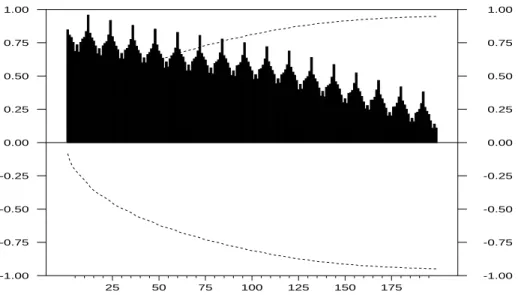
Two main stylized facts emerge strongly from this raw series, namely trend and seasonality, as it can be seen on the empirical ACF of the series on fig-ure 2. The empirical ACF is striking insofar it shows a slow decay, at an hyperbolic rate, as well as a seasonal pattern with a period of 12 months, corresponding to the sample frequency. If we look at the spectral density of the series estimated by the raw periodogram (see figure 3), we identify 7 peaks corresponding to the frequencies λj = 2πj/12, for j = 0, . . . , 6. The
zero frequency partly represents the long-term cycle, while other frequencies refer to the seasonal components of the series. Other features of this series may be also of interest for statistical analysis, like high volatility, increase in
25 50 75 100 125 150 175 -1.00 -0.75 -0.50 -0.25 0.00 0.25 0.50 0.75 1.00 -1.00 -0.75 -0.50 -0.25 0.00 0.25 0.50 0.75 1.00
Figure 2: ACF of the new car registration series in the euro area from Jan. 1960 to Dec. 2005.
0 pi/6 pi/3 pi/2 2 pi/3 5 pi/6 pi
0 2e+11 4e+11 6e+11 8e+11 1e+12 1.2e+12
Figure 3: Raw periodogram of the new car registrations series in the euro area from Jan. 1960 to Dec. 2005.
the variance or outliers due to the legislation on catalytic converters in 1993.
Let’s denote (Xt)t the raw series of new car registrations, for t = 1, . . . , T ,
with T = 552 observations. We discuss now the different models fitted to this data set. The results of the different tests are given in Table 1, as the values estimated for long memory parameters of the different models.
• First, we consider the classical filter generally used in papers dealing with applications of linear SARIMA processes, that is F (B) = (I − B)(I −Bs), with s = 12 for monthly data. This filter has been proven to
be useful to make vanish trend and seasonality. However, there always exists a risk of over-differenciation implying thus a loss of information. In this respect, fractional filters avoid over-differenciation by allowing to the differenciation degree to belong to the interval [0, 1].
• Secondly, we consider the ARFISMA filter F (B) = (I − B)d(I − Bs)D,
introduced previously in (14), d ∈ R, being the degree of integration of the long-term cycle and D ∈ R being the degree of integration of the seasonal part. All the results for different d and D, including d = 0 and D = 0, are presented in table 1, as well as the values of the statistics used to compare the models. Five different filters have been considered. we compare their accuracy through the values obtained for the statistics (21) and (22).
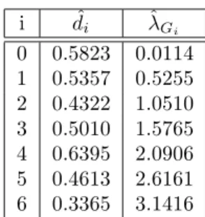
• Finally, we compare the previous fractional seasonal filters with a gen-eralized long memory approach. That is, we start from the empirical observation of the estimated spectral density exhibiting 7 peaks lo-cated at the seasonal frequencies. Thus, we propose a 7-factor Gegen-bauer process, described in the equation (5), the G-frequencies being λGj = 2πj/12, for j = 0, . . . , 6. The estimation step is thus reduced
to the estimation of the memory parameters dj for j = 0, . . . , 6. Here
again, the Whittle Pseudo-Maximum-Likelihood method is carried out to estimate those parameters. The simplex algorithm is used first to determine more precisely the initial values, then the BHHH algorithm
Filter F(B) dˆ Dˆ σˆε JB stat Q(12) Q(24) Q(60) Q(120) M1 = (I − B)(I − Bs ) 78689 522 185 340 696 1362 M2 = (I − B)d (I − Bs ) 0.3368 63556 268 71 162 366 735 M3 = (I − Bs)D(I − B) 0.6561 68133 214 161 311 712 1520 M4 = (I − B)(I − Bs )D 0.8924 76074 565 184 348 730 1454 M5 = (I − Bs)(I − B)d 0.6014 66749 506 114 239 526 1050 M6 = (I − B)d (I − Bs )D 0.6892 0.5894 62579 474 139 284 635 1332 M7 = GG7 58721 114 46 131 330 661
Table 1: Analysis of stochastic, ARFISMA and Gegenbauer filters applied on the new car registrations series in the euro area from Jan. 1960 to Dec. 2005, using empirical variances, JB and Portmanteau statistics. Estimation of the parameters d, D,for the stochastic and the ARFISMA filters.
i dˆi λˆGi 0 0.5823 0.0114 1 0.5357 0.5255 2 0.4322 1.0510 3 0.5010 1.5765 4 0.6395 2.0906 5 0.4613 2.6161 6 0.3365 3.1416
Table 2: Parameter estimation of parameters of the 7-factor Gegenbauer process adjusted on the new car registrations series in the euro area from Jan. 1960 to Dec. 2005.
is employed. Parameter estimates of the GG7 model are presented in table 2 significatively different from zero, but four of them imply a non-stationarity in some G-frequencies (for j = 0, 1, 3, 4). In Table 1 we give also the results for the statistics (21) and (22).
Comparing those seven models through the results given in Table 1, we ob-serve that the 7-factor Gegenbauer process provides the smallest residual variance implying thus a better fit to the data. Note however that this
M7 M1 M6 ˆ φ0 16485 (7.31) ˆ φ1 -0.2225 -0.6601 -0.0854 (-4.73) (-14.80) (-1.78) ˆ φ2 -0.3715 (-8.31) ˆ a0 0.8213 0.7499 0.7432 (13.63) (12.77) (12.62) ˆ a1 0.1479 0.2350 0.2360 (3.63) (5.60) (4.89) Q(3) 1.91 6.05 26.0 Q(6) 5.72 22.2 36.3 Q(12) 19.0 83.4 65.7 Skewness 0.0951 -0.2952 -0.2392 Kurtosis 0.6609 0.9724 0.8533 JB stat 8.51 23.29 17.23
Table 3: Estimates and standard errors of the parameters for the model (23) adjusted on the residuals of the 7-Gegenbauer process proposed for the new car registrations series in the euro area from Jan. 1960 to Dec. 2005.
model contains 7 parameters, instead of maximum 2 for the others models. Now, the Jarque-Bera statistics is also the smallest for the 7-factor Gegen-bauer process, albeit significantly different from zero at the usual type I risks, implying thus non-Gaussianity. The reduction of the JB statistics is equally due to a reduction of both skewness and kurtosis for this last model. Lastly, the Ljung-Box statistics is also strongly reduced for each K using the 7-factor Gegenbauer process. Consequently the 7-factor Gegenbauer process improves all the criteria and reproduces correctly both the seasonality and the persistence observed in the data.
For none of these models, the residuals are white. In order to whiten the residuals of the filtered series, we apply short memory filter on the residuals (εt)t. Thus, we fit a short memory process with conditional heteroscedasticity
(ARMA-GARCH type process) to the series (εt)t. We apply an
ARMA(2,0)-GARCH(1,0) process whose expression is given by:
εt = φ0+ φ1εt−1+ φ2εt−2+ ηt, ηt = htδt, (23) h2 t = a0+ a1ε 2 t−1, (24)
where (δt)t is a white noise process. We present the results for residuals
ob-tained through three of the previous models: the Models M1, M6 and M7. We observe that the 7-factor GIGARCH model M7 for which we fit on the filtered series a AR(1)-ARCH(1) process, is able to provide a Gaussian white noise residuals time series (δt)t, while the two others are not.
In conclusion, to describe the evolution of the new car registrations series in the euro area from January 1960 to December 2005, we retain the model described by the three following equations (values of ˆλGi and ˆdiare presented
in table 2): 7 Y i=0 (I − 2 cos(ˆλGi)B + B 2 )dˆiX t= εt, εt= 16485 − 0.2225εt−1+ ηt, ηt = δt q 0.8213 + 0.1479ε2 t−1,
3.2
Sales in the intermediate goods sector
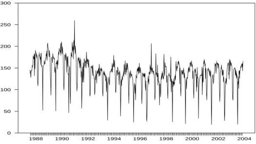
In this section, we consider the weekly sales of a big French company in the intermediate good sector from January 1988 to the end of May 2004, that is 854 observations, denoted (Yt)t=1,...,T. The series is presented in
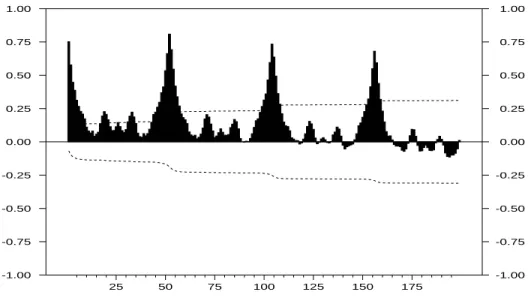
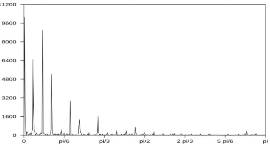
fig-ure 4. We observe evidence of a strong seasonal pattern as well as a pretty smooth trend. This pattern is confirmed by the graphs of the ACF in figure 5. The raw periodogram presented in figure 6 exhibits several peaks, specifi-cally for frequencies lower than π/3. Those peaks are located at the null and weekly seasonal frequencies, namely λh = 2πh/s, for h = 0, 1, 2, . . . , [s/2]
with s = 52. However, only the peaks associated to the first 7 frequencies can be clearly seen on the raw periodogram.
As in the previous application, our first aim is to filter this series to get a filtered series as white as possible and possibly Gaussian. We start by comparing fractional and linear filters, as regards trend and seasonality.
• Linear filters. The first filter we apply is the seasonal differentiation ∆s = (I − Bs), with s=52. The ACF of the filtered series is presented
in figure 10. This ACF shows two stylized facts: a slow decay for the first lags, indicating a strong degree of persistence, as well as a strong correlation at lag number 52, indicating the need for a short memory seasonal component. 1988 1990 1992 1994 1996 1998 2000 2002 2004 0 50 100 150 200 250 300
Figure 4: weekly sales of a big French company in the intermediate good sector from January 1988 to the end of May 2004.
25 50 75 100 125 150 175 -1.00 -0.75 -0.50 -0.25 0.00 0.25 0.50 0.75 1.00 -1.00 -0.75 -0.50 -0.25 0.00 0.25 0.50 0.75 1.00
Figure 5: ACF of the weekly sales of a big French company in the intermediate good sector from January 1988 to the end of May 2004.
1. To make vanish the slow decay, we consider first the classical linear filter ∆ = (I − B) on the filtered series that is we use the filter ∆∆s on the raw data (Yt)t.:
(I − B)(I − Bs)Yt= νt (25)
2. Second, to avoid over-differentiation we fit a fractional filter to the filtered series (εt)t, that is we use the filter ∆d∆s on the raw data
(Yt)t:
(I − B)d(I − Bs)Yt= δt (26)
We get the estimated memory parameter ˆd = 0.2834, implying thus the presence of stationary long memory.
Thus, comparing the models (25) and (26) and the value obtained for ˆ
d , this last result points out the over-differentiation due to the linear filter ∆.
• Fractional rigid filter.
1. We start by filtering first the raw series (Yt)tthrough the fractional
seasonal filter ∆D
s = (I − Bs)D introduced in (12). We get the
estimated value ˆD = 0.6671. The ACF (figure 11) of the filtered series (∆Dˆ
s Yt)t is very similar to the one of the seasonally filtered
0 pi/6 pi/3 pi/2 2 pi/3 5 pi/6 pi 0 1600 3200 4800 6400 8000 9600 11200
Figure 6: Raw periodogram of the weekly sales of a big French company in the interme-diate good sector from January 1988 to the end of May 2004.
2. However, if we apply a fractional filter to the filtered series (∆Dˆ s Yt)t,
the estimated memory parameter is higher than before and non-stationary ˆd = 0.6111, that is we consider the following model:
(I − B)0.6111(I − Bs)0.6671Y
t= εt. (27)
Note that the sum ˆd+ ˆD is very close using the previous fractional models :
1 + 0.2834 = 1.2834 and 0.6111 + 0.6671 = 1.2782, (28) but it is lower than the global degree of integration of the ∆∆s
filter (25) (equal to 2).
This phenomena is perhaps due to the Whittle estimation procedure which includes all the frequencies in the maximization algorithm. A non-parametric estimation procedure should be more appropriate for this kind of data. It could be interesting to compare both estimation procedures on this data set. Now, For the same last fractional filter ∆D
s∆d, if we estimate simultaneously both fractional parameters, d and
D, we get the following results : ˆD = 0.4444 and ˆd = 0.5366. The val-ues obtained are thus slightly lower, especially the seasonal fractional part of the model is now stationary. This results underlines the impor-tance of the parameter estimation method in the presence of both frac-tional trend and seasonality: particularly, the allocation of the memory
between those two parts has to be further investigated.
• According to the shape of the raw periodogram, it seems natural to try to fit a k-factor Gegenbauer to the raw series (Yt)t. Therefore,
we estimate a 7-factor Gegenbauer process with the G-frequencies cor-responding to the highest peaks in the raw periodogram, using the Whittle estimation method. We observe that all memory parameters are close to 0.1. However, after removing those components, there is still a seasonality in the filtered data, as it can be seen in the peri-odogram of the filtered series (see figure 12). Indeed, to remove all the seasonality through a k-factor Gegenbauer process, we should have used 53 factors, which is not reasonable, in particular with respect to the parcimony principle.
This application shows that, in this latter case, an ARFISMA model seems more appropriate to take the persistence in the seasonality, or in the cycle, into account. Indeed, it is untractable in practice to use a k-factor Gegen-bauer process as soon as the number of frequencies is too high. Moreover, we pointed out that the use of fractional filters for both trend and seasonality avoid over-differentiation.
4
Conclusion
Many economic time series display seasonal fluctuations linked to a kind of persistence, but it does not exist a single way to model the seasonal compo-nents and the long-term cycle. In this paper, we recall most of the different seasonal fractionally integrated processes which model trend and seasonality. We show that, on two applications on real data of the economic activity in the euro area, ARFISMA and k-factor GARMA processes offer very compet-itive alternatives to classical linear SARIMA processes, in the sense that they avoid over-differentiation while providing a better goodness of fit. We raise also the question of the "best" estimation procedure. This issue appears to be further investigated.
References
[1] Anderson, O.D. (1979) The autocovariance structures associated with general unit circle non-stationary factors in the autocovariance operators of otherwise stationary ARMA time series models, Cahiers du CERO, 21, 221 - 237.
[2] Arteche J. (2003) Semi-parametric robust tests on seasonal or cyclical long memory time series, Journal of Time Series Analysis, 23, 251 - 285.
[3] Arteche J., Robinson P.M. (2000) Semiparametric inference in seasonal and cyclical long memory processes, Journal of Time Series Analysis, 21, 1 - 25.
[4] Carlin, J.B., Dempster A.P. (1989) Sensitivity analysis of seasonal adjustements: Empirical cas studies, Journal of the American Statistical Association, 84, 6 - 20. [5] Chan N.H., Palma W. (2005) Efficient estimation of seasonal long range dependent
processes, Journal of Time Series Analysis, 26, 863 - 892.
[6] Chung C-F. (1996) A generalized fractionally integrated autoregressive moving av-erage process, Journal of Time Series Analysis, 17, 111-140.
[7] Darné O., Guiraud V., Terraza M. (2004) Forecast of the seasonal fractional inte-grated series, Journal of Forecasting, 23, 1 - 17.
[8] Diongue A. K., Guégan D. (2004) Forecasting electricity spot market prices with a k-factor GIGARCH process, Note de recherché MORA - IDHE - nř 9-2004, Décembre 2004, Cachan, France.
[9] Franses P.H., Ooms M. (1997) A periodic long memory model for quartely UK in-flation, International Journal of Forecasting, 13, 117 - 126.
[10] Ferrara, L. and D. Guégan (2000) Forecasting financial time series with generalized long memory processes, in Advances in Quantitative Asset Management, p.319-342, C.L. Dunis eds., Kluwer Academic Publishers.
[11] Ferrara, L. and Guégan, D. (2001a), Forecasting with k-factor Gegenbauer processes: Theory and applications, Journal of Forecasting, 20, 581-601.
[12] Ferrara, L. and D. Guégan (2001b), Comparison of parameter estimation methods in cyclical long memory time series, in Developments in Forecast Combination and Portfolio Choice, Chapter 8, C. Dunis, J. Moody and A. Timmermann (eds.), Wiley, New York.
[13] Giraitis, L., Leipus R. (1995) A generalized Fractionally Differencing Approacg in Long Memory Modelling, Lithuanian Mathematical Journal, 35, 65 - 81.
[14] Geweke J., Porter Hudak S. (1983) The estimation and application of long memory time series models, Journal of Time Series Analysis, 4, 67 - 90.
[15] Gil-Alana L.A. (2001) Testing stochastic cycles in macro-economic time series, Jour-nal of Time Series AJour-nalysis, 22, 411 - 430.
[16] Giraitis, L. and Leipus, R. (1995), A generalized fractionally differencing approach in long memory modeling, Lithuanian Mathematical Journal, 35, 65-81.
[17] Granger C.W.J. and R. Joyeux (1980) An introduction to long memory time series models and fractional differencing, Journal of Time Series Analysis, 1, 15 - 29.
[18] Grassman, P. and F. Keereman (2001), An indicator-based short-term forecast for quarterly GDP in the euro area, Economic Paper 154, European Commission. [19] Gray, H.L., Zhang, N.-F. and Woodward, W.A. (1989), On generalized fractional
processes, Journal of Time Series Analysis, 10, 233-257.
[20] Guégan, D. (2000), A new model : the k-factor GIGARCH process, Journal of Signal Processing, 4, 265-271.
[21] Guégan, D. (2003, A prospective study of the k-factor Gegenbauer process with heteroscedastic errors and an application to inflation rates, Finance India, 17, 1 - 21. [22] Guégan D., Ladoucette S. (2001) Non mixing properties of long memory processes,
CRAS Paris, t. 332, Série I, 1-4.
[23] Hassler U. (1994) Misspecification of long memory seasonal time series, Journal of Time Series Analysis, 15, 19 - 30.
[24] Hosking J.R.M., (1981), Fractional differencing, Biometrika, 68, 1, 165-176.
[25] Huang D., Anh V.V. (1993) Estimation of the non-stationary factor in ARUMA models, Journal of Time Series Analysis, 14, 27 - 46.
[26] Olhede S.C., McCoy E.J., Stephens D.A. (2004) Large-sample of the periodogram estimator of sesonally persistent processes, Biometrika, 91, 613 - 628.
[27] Porter-Hudak, S. (1990) An application to the seasonally fractionally differenced model to the monetary aggregates, Journal of the American Statistical Association, 85, 338 - 344.
[28] Ray B.K. (1993) Long-range forecasting of IBM product revenues using a seasonal fractionally differenced ARMA model, International Journal of Forecasting, 9, 255 -269.
[29] Reisen, V.A., A.L. Rodrigues, and W. Palma (2004) Estimation of seasonal fraction-ally integrated processes, mimeo.
[30] Robinson P.M. (1994) Efficient tests of non-stationary hypotheses, Journal of the American Statistical Association, 89, 1420 -1457.
[31] Woodward, W.A., Cheng Q.C. and Gray H.L. (1998) A k-factor GARMA long-memory model, Journal of Time Series Analysis, 19, 5, 485-504.
0 pi/6 pi/3 pi/2 2 pi/3 5 pi/6 pi 0 1e+09 2e+09 3e+09 4e+09 5e+09 6e+09 7e+09 8e+09 9e+09
Figure 7: Raw periodogram of the filtered series from 7-factor Gegenbauer process.
Square Root of Estimated Conditional Variance
1970 1973 1976 1979 1982 1985 1988 1991 1994 1997 2000 2003 0.80 0.96 1.12 1.28 1.44 1.60 1.76 1.92 2.08
Figure 8: Estimated conditional variance from the AR(1)-ARCH(1) process applied to the filtered series from the GG-7 process.
1970 1973 1976 1979 1982 1985 1988 1991 1994 1997 2000 2003 -4 -3 -2 -1 0 1 2 3 4
Figure 9: Standardized residuals of the AR(1)-ARCH(1) process applied to the filtered series from the GG-7 process.
25 50 75 100 125 150 175 -1.00 -0.75 -0.50 -0.25 0.00 0.25 0.50 0.75 1.00 -1.00 -0.75 -0.50 -0.25 0.00 0.25 0.50 0.75 1.00
Figure 10: ACF of the seasonally differenced weekly sales of a big French company in the intermediate good sector from January 1988 to the end of May 2004.
25 50 75 100 125 150 175 -1.00 -0.75 -0.50 -0.25 0.00 0.25 0.50 0.75 1.00 -1.00 -0.75 -0.50 -0.25 0.00 0.25 0.50 0.75 1.00
Figure 11: ACF of the fractional seasonally differenced weekly sales of a big French company in the intermediate good sector from January 1988 to the end of May 2004.
0 pi/6 pi/3 pi/2 2 pi/3 5 pi/6 pi
0 100 200 300 400 500 600 700
Figure 12: Periodogram of the GG7-filtered series of weekly sales of a big French company in the intermediate good sector from January 1988 to the end of May 2004.