HAL Id: hal-00446594
https://hal.archives-ouvertes.fr/hal-00446594
Submitted on 13 Jan 2010
HAL is a multi-disciplinary open access
archive for the deposit and dissemination of
sci-entific research documents, whether they are
pub-lished or not. The documents may come from
teaching and research institutions in France or
abroad, or from public or private research centers.
L’archive ouverte pluridisciplinaire HAL, est
destinée au dépôt et à la diffusion de documents
scientifiques de niveau recherche, publiés ou non,
émanant des établissements d’enseignement et de
recherche français ou étrangers, des laboratoires
publics ou privés.
Self Organizing Star (SOS) for health monitoring
Etienne Côme, Marie Cottrell, Michel Verleysen, Jérôme Lacaille
To cite this version:
Etienne Côme, Marie Cottrell, Michel Verleysen, Jérôme Lacaille. Self Organizing Star (SOS) for
health monitoring. European conference on artificial neural networks„ Apr 2010, Bruges, Belgium.
pp.99-104. �hal-00446594�
Self Organizing Star (SOS) for health monitoring
E. Cˆome1
, M. Cottrell1
, M. Verleysen2
and J. Lacaille3
1- Universit´e Paris I, SAMOS-MATISSE, UMR CNRS 8174 90 rue de Tolbiac, F-75634 Paris Cedex 13 - France 2- Universit´e Catholique de Louvain, Machine Learning Group
Place du levant 3, 1348 Louvain-La-Neuve - Belgium 3- Snecma, Rond-Point Ren´e Ravaud-R´eau,
77550 Moissy-Cramayel CEDEX - France
Abstract. Self Organizing Maps (SOM) have been successfully applied in a lot of real world hard problems since their apparition. In this paper we present new topologies for SOM based on a planar graph. The design of a specific graph to encode prior information on the dataset topology is the central question addressed in this paper. In this context, star-shaped graphs are advocated for health monitoring applications, leading to a new kind of SOM that we denote by Self Organizing Star (SOS). Experiments using aircraft engine measurements show that SOS lead to meaningful and natural dataset representation.
1
Introduction
SOM are well-known data mining tools which are frequently used to project high-dimensional data into a low-dimensional discrete space for visualization and exploratory purpose. In the context of dimensionality reduction, SOM can be thought as a kind of nonlinear but discrete PCA. SOM are classically defined by two key elements: a set of prototype vectors {m1, . . . , mK}, which are
d-dimensional vectors, d being the d-dimensionality of the dataset {x1, . . . , xn} and
a lattice or grid which defines a neighborhood relation between the prototypes. This lattice plays the role of the embedding space. Each unit or prototype is associated with a fixed position in this lattice or grid. Self-organization means that after convergence prototypes which are close in the lattice (with a small distance between them) will also be close in the data space. New data can be projected after learning of the SOM by affecting them to the location on the map of the best matching unit (BMU): the closest prototype vector to the datapoint. In this paper we investigate the opportunity of using other lattices different from regular rectangular or hexagonal grids defined thanks to undirected graphs, which will have the additional interesting property of being planar. By using such graphs all the interesting properties of SOM are kept, in particular easy data visualization and data exploration with the additional freedom of designing lattices more suited to the expected dataset topology. We also show how such graph can be designed in the context of a health monitoring application. The classical lattices for SOM are rectangular or hexagonal grids. Extensions of these classical topologies have already been investigated by several authors. Toroidal or spherical maps [1, 2], growing grid with free topology [3], and tree structured
SOM (to speed up computational time required for BMU search) [4, 5], among others. We follow here a path more similar to [6] which focuses on the use of graphs to define SOM topologies. Our solution differs from [6] by the nature of the graph being used for defining the SOM topology. We promote in particular the star topology, which leads to the method proposed here and called Self Organizing Star (SOS).
The paper is organized as follow. In Section 2 the basics of SOM will be reminded and the question of how the neighborhood relationship induced by a lattice influences the results of the algorithm will be addressed. The use of undirected graphs to define new lattices will also be investigated. In Section 3, the SOS solution proposed to deal with health monitoring problems will be advocated and described. Finally, some experimental results on real and sim-ulated datasets will be given using such a topology; the paper ends with some concluding remarks.
2
Self-Organizing Maps Background
In its classical presentation [7, 8], the SOM algorithm is an iterative algorithm, which iterates the two following steps over training patterns xj for computing
the set of prototypes mi, i ∈ {1, . . . , K} which define the map:
• Competitive step, this step aims at finding the best matching unit (BMU) for sample xj :
c = arg min
i∈{1,...,K}||xj− mi||. (1)
• Cooperative step, this step aims at moving the BMU and close units, closer to the training pattern:
mi(t + 1) = mi(t) + α(t)hci(t) [xj− mi(t)] , (2)
with t the time step, α(t) the learning rate of the algorithm and hci(t) the
neighborhood function between units c and i at time t. Several neighborhood functions are commonly used such as:
hci(t) = 1(dci<σt) (3)
hci(t) = exp(−d2ci/2σ2t). (4)
All of them depend on a radius σt which is classically decreasing during the
learning process. These neighborhood function also depends on dci: the distance
between neuron c and i, which is determined by the map topology. During the cooperative step the coordinates of the best matching unit c are updated in order to move it closer to the training pattern. Other prototypes mi are also
moved towards the training pattern according to their distance dcifrom the BMU
defined by the lattice. Closer units from the BMU will be more affected than the others. The two steps are iterated over the dataset during several epochs until
convergence. Convergence is being monitored by moves of prototype vectors. The learning rate is classically decreased during the learning process using an inverse linear adaptation. Thanks to the cooperative steps, auto-organization is reached at the end of the algorithm.
Looking at this algorithm, one can clearly see that the distance between units in the map plays a key role in the auto-organization property of the algorithm; therefore modifications of this distance will clearly have an impact on the re-sults of the algorithm. The lattice structure can be a way to incorporate prior information concerning the dataset topology into the dimensionality reduction process. In the context of classical SOM, one assumes that the dataset topology can effectively be represented by a grid or a straight line but other hypotheses can be interesting and can advantageously be investigated. The key element that implicitly or explicitly defines the lattice is the distance between map units. It has been already noted that graph theory can be used to define such distance [6, 4]. In this case, map units are the nodes of a graph, and distances between them are defined as the minimum number of edges needed to reach one node starting from the other, that is the so called shortest path distance.We therefore propose to modify the SOM algorithm only by taking as input an adjacency matrix which specifies the graph topology that the user desires. All undirected graphs can theoretically be used, but a specific class is of interest: the class of planar graph, because such graphs can easily be represented in a 2-dimensional setting allowing us to supply the SOM with visualization tools, as seen in the next section.
3
Star topology
In health monitoring applications, there exists a particular state which corre-sponds to the normal operation of the component under monitoring. The aim of health monitoring is to look at departures from this normal state, because faults lead to deviation of state variables from this normal state. Furthermore, we may hope that different faults are characterized by different shapes of drifts. The classical lattices of SOM do not take into account this prior information on
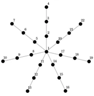
Fig. 1: Planar graph representation of the star topology with 7 rays and 3 units by rays
the dataset topology: there is no specific unit which takes a central place on the map. Moreover the users do not easily understand the meaning of the map since the normal states can for example be represented by codebooks vectors located on an edge of the map, instead of a central position that would be more natural. To prevent this difficulty, we propose to use a star-shaped graph as shown in Figure 1. This graph has a clear natural center from which different arms or rays grow. Such graph can easily be understood by users if different rays corre-spond to different faults and distances to the center describe the seriousness of the problem. These graphs can be characterized by their number of rays and by the length of the rays. SOM using such topologies will be called Self-Organizing Stars (SOS).
4
Results
4.1 Toy dataset
The first experiment aims at demonstrating the ability of such topology to rep-resent a star-shaped dataset. For this purpose a toy dataset was generated in a 3-dimensional space. One hundred data points have been generated using a normal distribution with mean (0, 0, 0) and standard deviation 2.I, where I de-notes the identity matrix of size 3 × 3. Three other sets of one hundred data points have been drawn, each corresponding to a noisy version of the segment [0, 15] along one of the three vectors of the R3 canonical basis. These sets were
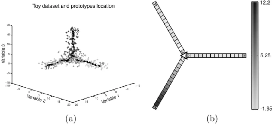
obtained by first sampling the location along the vectors using a uniform distri-bution between 0 and 15 and by adding isotropic noise with standard deviation equal to 1. A realization of such a dataset is presented in Figure 2 (a) with
5.25 12.2 -1.65 1 31 16 46 2 17 32 (a) (b)
Fig. 2: (a) toy dataset in R3 and SOS codebook’s position after learning
de-picted by big black dots, (b) Variable 1 component plane; map units colors are proportional to the first value of their codebooks vectors.
the SOS codebooks positions after learning. These results were obtained using a SOS with 3 rays of 15 units each. The training was performed using the classical
inverse linear learning rate scheme of SOM algorithms and a decreasing radius between 5 and 1; the number of epochs of the algorithm was fixed to 5 and the initialization was performed using random assignments in the data range for all units. Figure 2 (b) gives a representation of map results in the form of a compo-nent plane. We can also see on this figure that one ray corresponds to the part of the dataset simulated along the first canonical vector. This two representations clearly show that such dataset can be effectively described by a SOS; moreover using the planar representation of the star graph, such a SOM can be effectively represented in a 2 dimensional way.
4.2 Health monitoring dataset
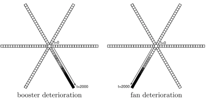
The second dataset comes from an health monitoring application which con-cerns aircraft engines. The data are multi-dimensional measurements on the engines (9 variables describing engines state and 7 variables describing the en-vironment). The dataset was simulated using a thermo-dynamical model of the engine; six different sets of points were simulated, each one starting from a nor-mal engine and gradually moving to a defective state. Such sets will be denoted as failure trajectory. Five sets concern progressive failures of different engine macro-components : fan, booster, high pressure core, high pressure turbine, low pressure turbine; the last one was generated with progressive degradation of all macro-components together. Random environmental conditions (external tem-perature, altitude, Mach, ...) were also simulated for all samples and finally realistic noise was added to all variables. Each one of the six sets contains 2000 points, leading to a dataset of 12000 multi-dimensional measurements. Rough engine measurements are inappropriate for direct use; they are indeed influenced by external conditions. We therefore first processed the data by a Linear Model (LM), to eliminate the effect of measured environmental conditions (external temperature, altitude, Mach, rotation speed, air levy, engine variable geometries positions) on the other 9 variables (temperatures and pressures on different loca-tions and fuel consumption). Finally, the LM residuals are filtered using a simple moving average (15 samples) in order to reduce noise. The filtered residuals are then used as inputs to a SOS for the easy visualization of fault degradations. The map was trained using an inverse linear scheme for the learning rate, 5 epochs and a neighborhood radius decreased from 5 to 1. The topology of the map was fixed manually: it contains 6 rays (one for each trajectory) of 20 pro-totypes each. Figure 3 presents the projection of two trajectories on the map. As expected each fault corresponds to a ray; similar results were obtained for the other faults. Once learned, the map is therefore a very interesting tool for health monitoring as it enables the diagnosis of specific sub-component failures and the estimation of the failure gravity.
5
Conclusion
The proposed SOM extension (SOS) based on a star shaped planar graph gives interesting results in the health monitoring application investigated in this paper.
booster deterioration fan deterioration
Fig. 3: Star-shaped map for turbo fan engine health monitoring; projection of the 2 first failure trajectories on the map; color (from white to black) and size (from small to big) of the squares indicates the position in the trajectory (from normal state to defective state).
This approach is interesting when prior information on the dataset topology is available as in health-monitoring applications. However, several questions are still open, first including the choice of the number of rays and their lengths which is left up to now to the user. Classical model selection tools can probably help for such a task. In addition, in the context of health monitoring applications we may face multiple simultaneous faults; this is not addressed by the proposed algorithm and is therefore also a topic for future work.
References
[1] Y. Wu and M. Takatsuka. Spherical self-organizing map using efficient indexed geodesic data structure. Neural Networks, 19:900–910, July 2006.
[2] G. Andreu, A. Crespo, and J. M. Valiente. Selecting the toroidal self-organizing feature maps (tsofm) best organized to object recognition. In Proceedings of International Con-ference on Artificial Neural Networks, Houston (USA), volume 1327 of Lecture Notes in Computer Science, pages 1341–1346, June 1997.
[3] B. Fritzke. Growing cell structures – a self-organizing network for unsupervised and su-pervised learning. Neural Networks, 7:1441–1460, 1994.
[4] J. Pakkanen, J. Iivarinen, and E. Oja. The elvoving tree - analysis and applications. IEEE Transactions on Neurals Networks, 17:591–603, 2006.
[5] M.M. Campos and G.A. Carpenter. S-tree: self organizing tree for data clustering and online vector quantization. Neural Networks, 14:505–525, 2001.
[6] A. Barsi. Neural self-organization using graphs. In Proceedings of the Third International Conference Machine Learning and Data Mining in Pattern Recognition, Leipzing (Ger-many), volume 2734 of Lecture Notes in Artificial Intelligence, pages 343–352. Springer, July 2003.
[7] T. Kohonen. Self-Organizing Maps. Information siences. Springer, 1995.
[8] M. Cottrell, Fort J.-C., and Pag`es G. Theoretical aspects of the som algorithm.